| Issue |
A&A
Volume 624, April 2019
|
|
|---|---|---|
| Article Number | A84 | |
| Number of page(s) | 9 | |
| Section | Stellar structure and evolution | |
| DOI | https://doi.org/10.1051/0004-6361/201834412 | |
| Published online | 15 April 2019 | |
Consistent accretion-induced heating of the neutron-star crust in MXB 1659−29 during two different outbursts⋆
1
Anton Pannekoek Institute for Astronomy, University of Amsterdam, Postbus 94249, 1090 GE Amsterdam, The Netherlands
e-mail: This email address is being protected from spambots. You need JavaScript enabled to view it.
2
Instituto de Astronomía, Universidad Nacional Autónoma de México, Mexico DF 04510, Mexico
3
International Centre for Radio Astronomy Research – Curtin University, GPO Box U1987, Perth, WA 6845, Australia
4
Department of Physics and Astronomy, Michigan State University, 567 Wilson Road, East Lansing, MI 48864, USA
5
Department of Physics & Astronomy, Wayne State University, 666 W. Hancock Street, Detroit, MI 48201, USA
6
Department of Physics and McGill Space Institute, McGill University, 3600 Rue University, Montreal, QC H3A 2T8, Canada
7
Department of Physics, University of Alberta, CCIS 4-181, Edmonton, AB T6G 2E1, Canada
8
SRON, Netherlands Institute for Space Research, Sorbonnelaan 2, 3584, CA Utrecht, The Netherlands
9
Eureka Scientific Inc., 2452 Delmer Street, Oakland, CA 94602, USA
10
Mathematical Sciences, University of Southampton, SO17 1BJ Southampton, UK
Received:
10
October
2018
Accepted:
4
March
2019
Abstract
Monitoring the cooling of neutron-star crusts heated during accretion outbursts allows us to infer the physics of the dense matter present in the crust. We examine the crust cooling evolution of the low-mass X-ray binary MXB 1659−29 up to ∼505 days after the end of its 2015 outburst (hereafter outburst II) and compare it with what we observed after its previous 1999 outburst (hereafter outburst I) using data obtained from the Swift, XMM-Newton, and Chandra observatories. The observed effective surface temperature of the neutron star in MXB 1659 − 29 dropped from ∼92 eV to ∼56 eV from ∼12 days to ∼505 days after the end of outburst II. The most recently performed observation after outburst II suggests that the crust is close to returning to thermal equilibrium with the core. We model the crust heating and cooling for both its outbursts collectively to understand the effect of parameters that may change for every outburst (e.g. the average accretion rate, the length of outburst, the envelope composition of the neutron star at the end of the outburst) and those which can be assumed to be the same during these two outbursts (e.g. the neutron star mass, its radius). Our modelling indicates that all parameters were consistent between the two outbursts with no need for any significant changes. In particular, the strength and the depth of the shallow heating mechanism at work (in the crust) were inferred to be consistent during both outbursts, contrary to what has been found when modelling the cooling curves after multiple outburst of another source, MAXI J0556−332. This difference in source behaviour is not understood. We discuss our results in the context of our current understanding of cooling of accretion-heated neutron-star crusts, and in particular with respect to the unexplained shallow heating mechanism.
Key words: accretion / accretion disks / stars: neutron / X-rays: binaries / X-rays: individuals: MXB 1659–29
A movie is available at https://www.aanda.org
© ESO 2019
1. Introduction
The density in the crust of a neutron star (NS) increases by several orders of magnitude over ∼1 km, from the upper layers of its outer crust to the crust-core boundary. Thus, NS crusts provide an excellent opportunity to study the behaviour of dense matter over a large density range. One of the ways in which we can do this is by studying the cooling of accretion-heated NS crusts. Several NSs in low-mass X-ray binaries (LMXBs; binary systems wherein the donor is typically a sub-solar star) experience transient outbursts during which matter from a disc around the NS is accreted onto its surface. This results in compression-induced exothermic nuclear reactions in the crust that can disrupt the crust-core thermal equilibrium (Haensel & Zdunik 1990, 2003, 2008; Steiner 2012). In these transient systems, the outbursts are separated by periods of quiescence during which no (or only very little) matter accretes onto the NS surface and as a result no (significant) heating by compression-induced reactions occurs. When such accretion outbursts have halted, the crust begins to cool in order to reinstate thermal equilibrium with the core (if this equilibrium was disrupted during the outburst). Monitoring this cooling has provided invaluable insight into the properties of matter over the high densities that occur in the NS crust, although many uncertainties remain (e.g. Shternin et al. 2007; Brown & Cumming 2009; see Meisel et al. 2018, for a review of the theoretical advances).
Currently, crust-cooling curves have been obtained for nine NSs in LMXBs (see Wijnands et al. 2017, for an observational review). Modelling these observed crust-cooling curves with theoretical models indicates that, besides the deep crustal heating mechanism (occurring deep in the crust, at densities of ρ ∼ 1012 − 1013 g cm−3), an additional, unknown crustal heat source should be active during the accretion outbursts of most sources to explain their early cooling evolution (e.g. Brown & Cumming 2009; Degenaar et al. 2014; Parikh et al. 2017a; Wijnands et al. 2017). This heat source is typically referred to as the shallow heating mechanism because as the name suggests it occurs at a shallower depth in the NS crust (i.e. at lower densities: ρ ∼ 108 − 1010 g cm−3) than the deep crustal heating.
MXB 1659 − 29 was discovered in 1976 (Lewin et al. 1976) as a transient LMXB that exhibited type-I X-ray bursts (which are caused by a runaway thermonuclear burning process on the NS surface) which established the NS nature of the accretor. The source was also found to exhibit eclipses, lasting ∼900 s, during its ∼7.1 h of orbit (Cominsky & Wood 1984; Jain et al. 2017; Iaria et al. 2018a). This outburst lasted ∼2–2.5 years (Wijnands et al. 2003). There were no follow-up observations to study the crust cooling of MXB 1659 − 29 after this outburst. A second accretion outburst from the source was detected in 1999 (in’t Zand et al. 1999) that lasted ∼2.5 years as well (Wijnands et al. 2002). Post-outburst observations (i.e. when the accretion had halted) using Chandra and XMM-Newton found a cooling NS crust (Wijnands et al. 2003, 2004; Cackett et al. 2006, 2008, 2013). This outburst is further referred to as outburst I as it was the first outburst in MXB 1659 − 29 after which crust cooling was investigated. MXB 1659−29 was the second source, after KS 1731−260 (Wijnands et al. 2003), for which such crust cooling was established. It was further monitored for up to ∼11 years after the end of this outburst until the source displayed a new outburst in 2015 (Negoro et al. 2015). The crust cooling of the NS in MXB 1659 − 29 monitored over this period, in addition to a similar monitoring of KS 1731−260 (e.g. Cackett et al. 2010; Ootes et al. 2016; Merritt et al. 2016), led to a significant leap in our understanding of the physics of the NS crust. Contrary to original expectation (Schatz et al. 2001), the NS crust in both sources was found to have a high thermal conductivity because it is likely a highly structured crystallised crust (with a low number of impurities; Shternin et al. 2007; Brown & Cumming 2009).
Following the long-term cooling of MXB 1659 − 29 allowed for the NS dense matter behaviour to be probed at all depths, from the topmost layers of the crust (Turlione et al. 2015; Horowitz et al. 2015; Deibel et al. 2017) to the core (Cumming et al. 2017; Brown et al. 2018), assuming we observed crust-core equilibrium again at the end of the available cooling curve (Cackett et al. 2013). However, this assumption may not be entirely valid since the interpretation of the results obtained during the last observations (Chandra observation IDs [obs IDs]: 13711 and 14453, carried out ∼3 days apart) after this outburst is ambiguous (see Cackett et al. 2013, for details): the decrease in count rate between these observations and the previous one could either be due to a further cooling of the crust, or to an increased internal absorption (e.g. due to an increase in the height of the outer accretion disc) with no further cooling of the crust. Neither scenario could be confirmed using additional observations since soon after the last observation the source exhibited its next accretion outburst. We assume that the most likely scenario is that of the increase in internal absorption meaning that the crust did not cool further. Therefore, we do not use these last two Chandra observations after outburst I in our study and we assume that the constant (plateau) level observed near the end of the cooling curve after outburst I is representative of the crust returning to thermal equilibrium with the core. Future quiescent observations after the end of its most recent outburst may help break the ambiguity of the interpretation of this last set of observations after outburst I (see Sect. 3).
MXB 1659−29 exhibited a new accretion outburst in 2015 (further referred to as outburst II; Negoro et al. 2015) which lasted ∼1.7 years, and the source transitioned back to quiescence in 2017 March (Parikh et al. 2017b). After the end of this outburst, we started a sequence of XMM-Newton and Chandra observations to obtain a second crust-cooling curve for this source. The early, preliminary cooling results, up to ∼26 days after the end of the outburst (and thereby probing only the upper layers of the crust), were reported by us in Wijngaarden et al. (2018). Here, we report on observations up to ∼505 days after the end of this outburst which allowed us to probe the physics of the deeper crust.
2. Observations, data analysis, and results
MXB 1659 − 29 is viewed at a high inclination (i ∼ 69–77°; Iaria et al. 2018a; Ponti et al. 2018) and eclipses are observed. To obtain the true intrinsic luminosity of the source (both during the outburst to estimate mass accretion rate variability (⟨Ṁ⟩) and during quiescence to determine the effective NS surface temperature [ ]) only the non-eclipsing “persistent” data should be used. Therefore, all data were corrected for eclipses using the ephemeris reported by Iaria et al. (2018a) by artificially reducing the exposure time corresponding to the number of the eclipses that occur during an observation. The eclipse lasts for ∼900 s of the ∼7.1 h orbital period of MXB 1659−29.
2.1. Light curves
Outburst I was observed using the All-Sky Monitor (ASM) aboard the Rossi X-ray Timing Explorer (RXTE). Data from the more sensitive RXTE/Proportional Counting Array (PCA) was used to track the end of outburst I. Outburst II was observed using the Gas Slit Camera (GSC) on board the Monitor of All-Sky X-ray Image (MAXI) and the X-ray Telescope (XRT) on board the Neil Gehrels Swift Observatory.
The 2–10 keV light curves1 obtained from the ASM and MAXI instruments were rebinned with a maximum of 4 days per bin to increase the data statistics. The data were further filtered such that points with error bars > 0.27 counts s−1 and > 0.28 counts s−1 were removed from the ASM and MAXI data, respectively. Examining the ASM light curve indicated that even when outburst I was over (based on the more sensitive PCA data as reported in a later paragraph and the first quiescent Chandra observation as discussed in Sect. 2.2.3) the source was detected at ≲0.7 counts s−1. Therefore, these ASM detections are not real and we removed all ASM data < 0.7 counts s−1 for these points. All MAXI data < 0.005 counts s−1 were removed to ensure that we only consider observations during which the source was conclusively detected.
Our raw Swift/XRT data (obs ID: 00034002001–00034002087)2 were processed using xrtpipeline (HEASOFT; v6.22). The background-corrected light curve was generated using XSelect (v2.4). A circular source region with a radius of 50″ centred on the source position was used (Wijnands et al. 2003). As background region we used an annulus (again centred on the source position) with an inner and outer radius of 175″ and 300″, respectively. The data were corrected for pile-up when necessary. All type-I X-ray bursts (found by visually inspecting the light curves) were removed from the data. In addition to eclipses, MXB 1659 − 29 also exhibits strong dipping behaviour preceding the eclipses (Cominsky & Wood 1984). Only when the data quality was high (e.g., during the outburst observations using the XRT) could these dips be discerned from the persistent flux in the light curves. The data were corrected for this dipping (by discarding the intervals) whenever they were clearly visible (by eye) in the light curves. Additionally, Wijnands et al. (2003) also observed dipping when the source was in quiescence. Thus, this dipping behaviour contributes a systematic source of uncertainty in quiescent observations (which is difficult to model).
Determining the date of the end of the outburst is important in our cooling model (Sect. 2.3). The source was last detected by the XRT during outburst II on MJD 57799.8. During the subsequent observation ∼20 days later the source was detected in quiescence at a count rate lower by a factor of ∼600. We assume that the outburst ended on MJD 57809.7, as determined by linearly interpolating between the date on which the source was last detected in outburst and subsequently detected at a lower level (lower by a factor ∼600) in quiescence, for the first time3.
We also determine the end of outburst I in the same manner, for consistency. Since the ASM is not very sensitive at the low count rates near the end of an outburst, we have used the data obtained from the PCA on board RXTE near the end of the outburst as reported by Wijnands et al. (2002). They found that the source was detected by the PCA on MJD 52159 at ∼5 mCrabs. Assuming, 1 Crab (2–60 keV) = 2.4 × 10⁻⁸ erg cm−2 s−1 (0.5–10 keV) we find that MXB 1659 − 29 was detected by the PCA at ∼1.2 × 10⁻¹⁰ erg cm−2 s−1. The source was not detected on MJD 52166 (with the upper limit corresponding to ≲1 mCrab (2–60 keV), i.e. ≲2.4 × 10⁻¹¹ erg cm−2 s−1 (0.5–10 keV)). Therefore, linearly interpolating between these dates we calculate MJD 52162 to represent the end of outburst I. This is different from the end of the outburst date assumed by Cackett et al. (2008) as they assumed that the last day on which the source was detected in outburst corresponded to the end of the outburst (MJD 52159.5). We have updated this assumption here, to be consistent with our analysis of outburst II.
The light curves described here are presented as bolometric flux curves in Fig. 1 (see Sect. 2.3 for details). Outburst I lasted for ∼2.5 years whereas outburst II lasted for ∼1.7 years. Outburst I transitioned smoothly from a constant flux level during the outburst to a rapid decay near the end of the outburst. Outburst II exhibited a lot more variability during the last ∼5 months and did not transition to the outburst decay as smoothly as observed for outburst I.
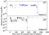 |
Fig. 1. Bolometric flux (0.01–100 keV) curves for outbursts I and II (upper and lower panels, respectively). The zero points correspond to MJD 51265 for outburst I and MJD 57256 for outburst II. The vertical grey dotted lines indicate the time of the end of the respective outbursts (MJD 52162 and MJD 57809.7, respectively). For outburst I, the ASM data are shown in blue and the PCA data near the end of the outburst (including the upper limit indicated by the downward facing triangle) are shown in magenta. For outburst II, the MAXI and XRT data are shown by open and filled black circles, respectively. The vertical red arrows in the lower panel indicate the times of the observations of the source in quiescence after the end of outburst II (see Sect. 2.2 and Table 1, for details). |
2.2. Post-outburst spectral analysis
We present five new observations of MXB 1659 − 29 after the end of outburst II, in addition to the two intervals reported by Wijngaarden et al. (2018). So far, MXB 1659 − 29 has been observed twice using XMM-Newton and four times using Chandra, up to ∼505 days after the end of this outburst. The early post-outburst II cooling evolution could be constrained by combining several Swift/XRT observations. In Sect. 2.3, we modelled the results obtained from the quiescent observations after both outbursts collectively to obtain the best constraints on the crustal physics. Therefore, for uniformity, we also reanalysed all the observations after the end of outburst I (Wijnands et al. 2003, 2004; Cackett et al. 2006, 2008, 2013) in the same way as for the observations performed after outburst II. The log of all the observations used in our paper is shown in Table 1.
Log of the quiescent observations used in our paper and results of the spectral fitting.
2.2.1. Swift/XRT
We combined five observations (obs ID: 00034002072–00034002076, as Interval 1) taken ∼10–18 days after the end of outburst II. The count rates from these observations were consistent with one another. The Photon Counting mode (2D imaging) event files from these observations were combined and the count rate and spectrum were extracted using a circular source region with a radius of 20″ centred on the source position. The same background region as used for the light-curve extraction was used (Sect. 2.1). The ancillary response file was constructed using the xrtmkarf tool. The response matrix file swxpc0to12s6_20130101v014.rmf, as indicated by the xrtmkarf tool, was used.
2.2.2. XMM-Newton
MXB 1659 − 29 was observed once after the end of outburst I and twice after the end of outburst II using all three XMM-Newton European Photo Imaging Cameras (EPIC) – pn, MOS1, and MOS2. The source was too weak to be detected significantly by the Reflection Grating Spectrometer, therefore, data from this instrument are not used. We do not use data from the Optical Monitor instrument as these are not useful for our cooling studies. The raw data4 were processed using the Science Analysis System (SAS; v16.1). The data (in the 10–12 keV energy range for the pn detector and > 10 keV for the MOS detectors) were examined for background flares. To discard these flares, data exceeding > 0.25 − 0.3 counts s−1 and > 0.2 − 0.3 counts s−1 were removed from the appropriate pn and MOS observations, respectively.
The source region used for the light curve and spectral extraction was calculated using the eregionanalyse tool to optimise the signal-to-noise ratio. Circular source regions (centred on the source position) with radii of 14.5″ − 18″ and 12″ − 18″ were recommended for the pn and MOS data, respectively. A circular background region with a radius of 50″ was used throughout. The location of the background region was recommended by the ebkgreg tool. The rmfgen and arfgen tools were used to create the response matrix files and ancillary response functions.
2.2.3. Chandra
Chandra was used to observe MXB 1659 − 29 eight times after outburst I and, so far, four times after outburst II. All the observations were carried out in FAINT mode and the source was positioned on the S3 chip of the Advanced CCD Imaging Spectrometer (ACIS). The data5 were reduced using CIAO (v4.9). A circular source-extraction region with a radius of 2″ and an annular background region with inner and outer radii of 10″ and 20″ (both centred on the source position), respectively, were used throughout for the light curve and spectra extraction. The data were examined for background flaring (by examining the light curve from the whole field of view excluding the region around the source) and only one observation (obs ID: 3795) showed such a flare. To correct for this episode of background flaring, data exceeding > 4.5 counts s−1 were removed from this observation. This reduced the useful exposure time of this observation from ∼27.1 ks to ∼25.6 ks.
The spectra were extracted using the specextract tool. This tool generates the source and background spectrum along with the redistribution matrix file and the aperture-corrected auxiliary response file. Two observations (obs ID: 5469 and 6337) were very close in time (∼1400 days and ∼1417 days after outburst I). We combined the spectra from these two observations to obtain better constraints from our spectral fitting using the combine_spectra tool6. The last two observations after the end of outburst I have not been included in our analysis (see Sect. 1, for details).
2.2.4. Spectral fitting
All the XMM-Newton and Chandra spectra were grouped to have a minimum of five counts per bin and the Swift/XRT Interval 1 spectrum was grouped to have a minimum of two counts per bin. The XMM-Newton spectra were grouped using the specgroup tool and the Chandra and XRT spectra using the grppha tool. Due to the low number of counts per bin for the various spectra, χ2 statistics could not be used for the spectral fitting. Therefore, all the spectra were fit collectively using XSpec (v12.9; Arnaud 1996) in the 0.3–10 keV energy range using W-statistics (background subtracted-Cash statistics; Wachter et al. 1979). Data after both outbursts were fitted collectively to obtain the best model constraints. We fit our spectra using the NS atmosphere model (nsatmos; Heinke et al. 2006) and assumed a NS mass and radius of 1.6 M⊙ and 12 km7. Analysis of the type-I bursts of MXB 1659 − 29 for hydrogen-rich and helium-rich material indicated distances of 9 ± 2 kpc and 12 ± 3 kpc, respectively (Galloway et al. 2008). We assume a distance (D) of 9 kpc8 We examined the Gaia archive and found that the source position coinciding with MXB 1659 − 29 was not accompanied by any stellar parallax information. Therefore, no distance constraint could be obtained using the Gaia data. We assume that the entire NS surface is emitting and set the related normalisation to 1 in the nsatmos model. The equivalent hydrogen column density (NH) was modelled using tbabs, employing VERN cross-sections and WILM abundances (Verner et al. 1996; Wilms et al. 2000).
We assume that the NH remained constant throughout and tie it across all the spectra9. The effective NS temperature was left free to vary across all the observations but was tied between the pn and MOS detectors for a given XMM-Newton observation. To account for the normalisation offset between the different observatories we used an additional constant component as has also been used in previous cooling studies (see Parikh et al. 2017c, for details). The value of this component was determined using Table 5 of Plucinsky et al. (2017, CXRT = 0.872, Cpn = 0.904, CMOS1 = 0.983, CMOS2 = 1, and CChandra = 1). No additional non-thermal component was needed to fit the spectra. All errors are stated for the 90% confidence level and all the measured effective temperatures are in terms of the effective surface temperature that would be seen by an observer at infinity10 ( ).
).
The best-fit NH was NH = (3.4 ± 0.2) × 1021 cm−2. The NH was fixed to this value before calculating the errors on the  to obtain a more precise result (for justification of this see, e.g. Wijnands et al. 2004; Homan et al. 2014; Parikh & Wijnands 2017). The results of the spectral fitting are shown in Table 1 and the
  evolution of the cooling crust is shown in Fig. 2.
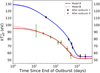 |
Fig. 2.
|

2.3. Modelling the  evolution
We model the  evolution of MXB 1659 − 29 after both outbursts I and II using the crust heating and cooling code NSCOOL (Page 2016). We account for the accretion rate variability during the outbursts in our model by using the observed variability in the bolometric flux (Fbol, 0.01–100 keV; Ootes et al. 2016, our code also allows for multiple outburst to be followed in this way; see Parikh et al. 2017c; Ootes et al. 2018 for details).
2.3.1. Modelling the mass accretion rate ⟨Ṁ⟩ during the outbursts
To obtain this Fbol, we use light curves (see Sect. 2.1, for details) from various instruments and determine appropriate count-rate-to-Fbol conversion factors. For outburst I, we use the 2–10 keV RXTE/ASM light curve and the more sensitive 2–10 keV RXTE/PCA observations near the end of the outburst. For outburst II, we use the 2–10 keV MAXI/GSC light curve as well as the 0.5–10 keV Swift/XRT data.
Recently Iaria et al. (2018b) reported the Fbol of MXB 1659 − 29 during high- and low-flux states during outburst II. They also showed that the source likely exhibited the same high-flux state (observed during outburst II) during outburst I as well (MJD 51961 and MJD 57499, respectively; see their Sect. 2.4). Since the source exhibits the high-flux state during most of both the outbursts we have only used the high-flux Fbol in determining our conversion factors for both outbursts I and II. The reported unabsorbed high-flux Fbol is 2.2 × 10⁻⁹ erg cm−2 s−1. This Fbol has been corrected for all bursts, eclipses, and dipping behaviour and is representative of the persistent emission of the source during the high-flux state.
The count-rate-to-Fbol conversion factors for the ASM, MAXI, and Swift have been determined using the count rate during the observation performed closest in time to the data from which Iaria et al. (2018b) obtained the Fbol. We ensure that the count rate corresponding to this observation is representative of the persistent emission from the source (and does not experience any bursts, eclipses, or dipping behaviour). The count-rate-to-Fbol conversion factors for the various instruments are: CASM = 1.0 × 10⁻⁹ erg cm−2 counts−1, CMAXI = 2.6 × 10⁻⁸ erg cm−2 counts−1 and CSwift = 1.4 × 10⁻¹⁰ erg cm−2 counts−1. A similar factor could not be determined for the PCA data near the end of outburst I since these data were not coincident with the time of the Fbol reported during this outburst. Instead, we used a correction factor of two (in’t Zand et al. 2007) to convert the 2–10 keV flux to the Fbol. These Fbol curves are shown in Fig. 1. The upper panel shows outburst I with the four-day binned and error filtered ASM data shown in blue and the PCA data (including the upper limit shown by a downward pointing triangle) in magenta. The lower panel shows the bolometric flux curve of outburst II with the MAXI data shown using the open black circles and the Swift/XRT data by the filled black circles. For outburst II, in cases when both MAXI and Swift data were available for the same day, the Swift data were preferred. The vertical grey dotted line in both panels indicates the end of the outburst. The vertical red arrows in the lower panel show the times of the quiescent observations (see Sect. 2.2 and Table 1; see Cackett et al. 2006, 2010, for the times of the quiescent observations after the end of outburst I).
These calculated Fbol curves were then used to determine the daily average accretion rate using
 (1)
(1)
where η (=0.2) indicates the efficiency factor and c is the speed of light. These Fbol curves were used to calculate the outburst fluence. The fluence for outbursts I and II was found to be ∼0.17 erg cm−2 and ∼5.18 × 10⁻² erg cm−2, respectively.
2.3.2. Modelling the neutron star heating and cooling
For consistency in our NSCOOL modelling, we used the same values of the NS mass and radius as assumed for the spectral analysis (see Sect. 2.2 and Appendix A for information about self-consistent modelling in NSCOOL). Both, the deep crustal heating as well as shallow heating were modelled. The contribution of deep crustal heating was fixed at 1.93 MeV nucleon−1 (Haensel & Zdunik 2008). The strength (Qsh) and the depth ( ρsh) of the shallow heating were model fit parameters. The additional model fit parameters were the column depth of light elements in the envelope11 (ylight), the initial red-shifted core temperature ( ) of the NS, and the impurity factor of the crust (Qimp) which was modelled as three layers12. Our model assumes that the Qimp in the different crustal layers remains the same between the two outbursts. The best fit was found using the χ2 minimisation technique.
Initially, we allowed the shallow heating parameters (Qsh and ρsh) and ylight to vary between the two outbursts, as it was found in studies of multiple cooling curves of other sources that these parameters could indeed be different between outbursts (i.e. not consistent with the error bars; Parikh et al. 2017c; Ootes et al. 2018). This is shown as Model A in Fig. 2 (by the solid curve; blue and red are used to indicate the cooling curves after outbursts I and II, respectively) and Table 2. The fit indicates that the Qimp in all the layers is low, with the best-fit indicating that Qimp ≲ 3 for all the three layers (with the lowest bound extending to 0). The fit values of the shallow heating parameters (active during the accretion outburst) and ylight (at the end of the outburst) during the collective modelling of the two outbursts are consistent with one another. The ylight is used to translate the boundary temperature at ρ = 108 g cm−3 into the temperature seen by an observer (see Fig. 1 of Ootes et al. 2018). Since the best-fit ylight for Model A is different after outbursts I and II the source reaches a different base level (as can be seen from Fig. 2 after ≳1000 days). However, the ylight values are consistent within the error bars and may still be the same after the two outbursts (as can be seen in Fig. 3a which shows the cooling curves of Model A along with its error bands). We can investigate this further using our upcoming Chandra observations. We have also modelled the source reaching the same base level (once the crust returns to equilibrium with the core) after both the outbursts as Model B (shown by the dotted curve in Fig. 2 and with its corresponding error band in Fig. 3b) by tying the ylight between the two outbursts. All fit parameter values between Models A and B are consistent (see Table 2).
Results of the NSCOOL model fits to the observed  evolution in MXB 1659 − 29 after outbursts I and II.
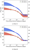 |
Fig. 3. Cooling curves modelling the |


We have also modelled the cooling evolution of the source assuming that the shallow heating parameters between the two outbursts are the same (as Model C, see Table 2). This gives, as expected, a similar result as seen for Model A, that is, ylight between the two outbursts is consistent and the Qimp is low. We do not show Model C in Fig. 2 because it almost entirely overlaps with Model A.
2.3.3. A look at the temperature profiles inside the neutron star
Using our NSCOOL model, we can also examine the evolution of the temperature profile in the NS crust during and after the end of both accretion outbursts in MXB 1659−29. This has been done for Model B, presented as Video 1 (see online material). Outburst I is indicated using blue and outburst II using red. The left panel shows the mass accretion rate variability during both the outbursts (shown as the effective temperature as a function of time). The upper-left and lower-left panels show outbursts I and II, respectively, and the zero point (shown by the vertical dotted line) indicates the time of transition to quiescence. The right panel shows the temperature profile in the neutron star and the dashed vertical line is indicative of the crust–core boundary. The temperatures in the right panel are the local, that is, non-redshifted, temperatures. The video has been presented such that both outbursts (although they have different lengths) transition to quiescence at the same time. This means that the accretion in outburst I starts before that in outburst II as outburst I is longer.
The temperature profile in the crust of a neutron star is set by the core temperature when the crust is in thermal equilibrium with the core. In our system, this crust–core equilibrium condition exists before and after the two accretion outbursts. The pre-outburst II profile is the profile in the crust after the end of outburst I (once the crust-core equilibrium has been re-established).
As the source begins to accrete the crust begins to heat up (seen as two bumps in the temperature profile) due to the two heat sources – the deep and shallow crustal heating. This heat spreads very quickly through the crust yielding a much smoother temperature profile. The profile in the outer crust is highly variable as the shallow heat source responds almost instantaneously to the outburst accretion rate variability.
The bump around the depth where deep crustal heating occurs is lower for outburst II than for outburst I as outburst II was shorter (with a smaller total accreted mass). It can be seen that the crust begins to cool as soon as the accretion stops. As seen from our observations, outburst I takes longer to achieve equilibrium with the core than outburst II.
3. Discussion
MXB 1659 − 29 is a LMXB that hosts a NS. We study the crust cooling of the NS crust in MXB 1659 − 29 after two accretion outbursts using data obtained from the Swift, XMM-Newton, and Chandra observatories. The two outbursts studied here – outburst I (1999–2001) and outburst II (2015–2017) had a similar peak flux but had different durations, lasting ∼2.5 years and ∼1.7 years, respectively. Experience from the previous outburst and theoretical expectations showed the importance of observations during the early cooling phase soon after the end of the outburst. For MXB 1659−29, we obtained a much improved coverage for the first ∼200 days after the end of outburst II as compared to outburst I.
We reduced and modelled all the quiescent crust cooling data collectively for consistency. We found that during outburst I the crust was heated up to a higher temperature than during outburst II, but after both outbursts the NS crust exhibited cooling. The post-outburst cooling, as inferred from our spectral fitting results, indicated a  drop from ∼111 eV to ∼55 eV from ∼36 days to ∼2422 days after the end of outburst I and from ∼92 eV to ∼56 eV from ∼12 days to ∼505 days after the end of outburst II. The
  extracted from the most recently performed observation after outburst II is consistent with the
  that was assumed to represent the crust-core equilibrium after outburst I (see Table 1 and Fig. 2). This suggests that the crust may be close to returning to thermal equilibrium with the core if the assumed base level after both outbursts is the same (see Model B). We will obtain at least two more Chandra observations of the source in the future (currently planned for 2019). This will provide us with information about whether the crust will cool further or not since it has re-established thermal equilibrium with the core.
Future observations in quiescence may also help break the ambiguity of the last observations after the end of outburst I (taken ∼3 days apart; see Sect. 1 and Cackett et al. 2013). Examining high-quality spectra taken at a similar time ∼11 years after the end of outburst II (if the source does not start a new accretion outburst before that) will allow us to infer if the base level does drop or if indeed the NH increases due to build up of material in the disc.
We have collectively modelled the cooling trend observed after outbursts I and II using our theoretical crust heating and cooling code NSCOOL (Page 2016; Ootes et al. 2016, 2018). We assumed that the impurity parameter Qimp in the crust does not vary between the outbursts. As is seen for several sources (Shternin et al. 2007; Brown & Cumming 2009; Page & Reddy 2013; Ootes et al. 2016), our models indicate a low Qimp (best-fit shows Qimp ≲ 6) in the crust, meaning a high thermal conductivity. Initially, we allowed both the shallow heating parameters (Qsh and ρsh) and the envelope composition (ylight) to vary between both the outbursts. Our models suggest that all our NSCOOL fit parameters are consistent between the two outbursts (although the absolute values of the parameters between the two outbursts may be different they are still consistent within the error on these values). This makes MXB 1659 − 29 a predictable cooling source whose quiescent cooling evolution after a new outburst can be calculated using information obtained from the cooling curve after a previous outburst. Wijngaarden et al. (2018, see their Fig. 1, right) reported the early post-outburst II cooling results of this source (from Interval 1 determined using the Swift/XRT data and the first XMM-Newton observation after the end of outburst II). We have obtained five additional observations of MXB 1659 − 29 since then. It is very interesting to note that the  determined from the five subsequent cooling observations are nicely consistent with the predicted cooling curve we showed in Wijngaarden et al. (2018). This prediction still holds true when the models are updated for our re-evaluated assumptions (see below) as the updated assumptions result in a revised contribution from the shallow heating which dominates the crust cooling behaviour observed so far after outburst II with very little influence from the deep crustal heating.
Our results, showing that MXB 1659 − 29 needs similar shallow heating during both its accretion outbursts, are not consistent with the results reported by Wijngaarden et al. (2018). This inconsistency is a result of the different Fbol assumed by Wijngaarden et al. (2018) for outburst I. The Fbol is used to determine the daily average accretion rate (see Eq. (1)) which in turn is used to determine the Qsh (which is assumed to be proportional to the accretion rate, see Eq. (1) of Ootes et al. 2018). The Fbol assumed by Wijngaarden et al. (2018, which was determined using WebPIMMS13) for outburst I was a factor of ∼2 lower than what we derived using the assumptions indicated in Sect. 2.3. This explains why Wijngaarden et al. (2018) found that outburst I needed a Qsh a factor of ∼2 higher than what we find for our model. Our assumption is more robust since it uses actual spectral fit values reported by Iaria et al. (2018b) to determine the Fbol.
Since the Qsh parameters for MXB 1659 − 29 are consistent between the two outbursts and both outbursts have very similar peak fluxes, we investigated the possibility that the Qsh may be related to the peak flux. To improve the statistics of our study, we only used the results of MAXI J0556−332 and Aql X−1 (Parikh et al. 2017c; Ootes et al. 2018) because these are the only other two sources for which multiple cooling curves have been collectively modelled. Studying these data we do not find any conclusive evidence that the Qsh may be related to the peak flux of the outburst.
Using our NSCOOL model we calculated the fluence of the two outbursts (see Sect. 2.3). We find that the fluence of outburst I was a factor of ∼3.3 higher than that of outburst II. Even though the two outbursts of MXB 1659 − 29 exhibited a different fluence, our modelling indicates that they need a similar Qsh. This is different from the shallow heating requirements of MAXI J0556−332 which indicated that different amounts of Qsh were required during its three accretion outbursts to explain their post-outburst cooling evolution and that the magnitude of the Qsh required seemed to be proportional to the outburst fluence (Parikh et al. 2017c). Our results are also different from those published by Wijngaarden et al. (2018). They reported that the Qsh was also proportional to the outburst fluence for MXB 1659−29. However, this is no longer true since (as shown earlier in this section) we robustly recalculated the fluence from MXB 1659 − 29 and remodelled the data resulting in a different contribution from the Qsh. Both the fluence and the Qsh were found to be different from those of Wijngaarden et al. (2018). This results in the Qsh no longer being proportional to the fluence for MXB 1659−29.
In our model, the total contribution from the shallow heating is assumed to be proportional to the outburst ⟨Ṁ⟩ variability, with each accreted nucleon contribution being Qsh MeV of heat. For MXB 1659−29, we found that the magnitude of heating needed per accreted nucleon (Qsh) was consistent during two different accretion outbursts. This shows that our assumption of the dependence of total shallow heating on the ⟨Ṁ⟩ variability is robust. However, this is only true for MXB 1659−29. MAXI J0556−332, another crust cooling source, needed different Qsh during its three outbursts to explain the cooling evolution observed in quiescence.
The origin and nature of the unknown shallow heat source remains a puzzle. However, studying more sources, including different outbursts of the same source, will increase the known constraints on the shallow heat source. Although a slow process, this currently seems to be one of only two proven ways forward (the other being studies using type-I bursts; e.g. Cumming et al. 2006; Linares et al. 2012; in’t Zand et al. 2012; Meisel et al. 2018) in allowing us to infer the physical origin of the shallow heat source. It is important to continue both these complementary studies to ensure that the Qsh requirements are consistent.
In their study of MXB 1659−29 after outburst I, Brown et al. (2018) show that the core temperature can evolve during both the accretion outburst and the crust relaxation phase and they moreover conclude that the long-term evolution of this NS requires the occurrence of fast neutrino emission in its inner core with an emissivity comparable to the direct Urca process. The timescale for significant core temperature changes after outburst I, from Fig. 1 of Brown et al. (2018), is of several years, significantly longer than the timespan of present observations after outburst II. It takes about 10 years of further cooling to result in a 6% change of effective core temperature compared to the 7.5% 1σ error of our last data point. When studying the impact of shallow heating, which is of importance during the early relaxation phase after the end of the accretion outburst, the response of the neutron star core is hence of very little relevance but will become an important issue in the future if further cooling of MXB 1659−29 after outburst II can be detected.
Movie
Video 1 Access Supplementary Material
The one-day binned light curves were obtained from the respective archives:
We also modelled the observed cooling evolution (see later sections) assuming the end of outburst was the last day on which the source was detected in outburst (MJD 57799.8) or, alternatively, the first day it was detected at a factor ∼600 lower level (MJD 57819.6), in quiescence. These two options constitute the two most extreme (albeit unlikely) possibilities for the exact end date of the outburst. We find that changing the end of outburst date does not change the broad physical interpretation of our results.
Obtained using the XMM-Newton archive: http://nxsa.esac.esa.int/nxsa-web/
Obtained using the Chandra archive: http://cda.harvard.edu/chaser/
This was not done during previously reported analyses of the source (Cackett et al. 2008). Using both the combined and non-combined data yields results consistent with one another.
We have also carried out the spectral fitting and NSCOOL modelling assuming a NS mass and radius of 1.4 M⊙ and 10 km, as was assumed for MXB 1659 − 29 for the post-outburst I cooling studies (Cackett et al. 2013). We find that this does not change the broad physical interpretation of our results.
We also investigated both the spectral analysis and the  modelling, assuming D = 12 kpc. The physical interpretation of our results remains the same.
We find that leaving the NH free for each observation results in the NH being consistent between all the observations we consider (since we do not include the last two observations after outburst I). Thus, this assumption is valid.
 , where (1 + z) is the gravitational redshift factor. For MNS = 1.6 M⊙ and RNS = 12 km, (1 + z)=1.29.
The envelope constitutes the outer NS where ρ < 108 g cm−3 and its composition determines how the temperature at the bottom of the envelope is translated to a surface temperature which is then measured by the observer (see also Ootes et al. 2018).
These layers correspond to the outer crust, the neutron drip layer, and the inner crust where the nuclear pasta is expected to occur (see Ootes et al. 2018, for details, as well as footnote b of Table 2).
Acknowledgments
AP, RW, LO, and ARE are supported by a NWO Top Grant, Module 1, awarded to RW. ND is supported by an NWO Vidi grant. DP is partially supported by the Consejo Nacional de Ciencia y Tecnología with a CB-2014-1 grant #240512. This work benefitted from support by the National Science Foundation under Grant No. PHY-1430152 (JINA Center for the Evolution of the Elements).
References
- Akmal, A., Pandharipande, V. R., & Ravenhall, D. G. 1998, Phys. Rev. C, 58, 1804 [NASA ADS] [CrossRef] [Google Scholar]
- Arnaud, K. 1996, Astronomical Data Analysis Software and Systems V, 101, 17 [NASA ADS] [Google Scholar]
- Brown, E. F., & Cumming, A. 2009, ApJ, 698, 1020 [NASA ADS] [CrossRef] [Google Scholar]
- Brown, E. F., Cumming, A., Fattoyev, F. J., et al. 2018, Phys. Rev. Lett., 120, 182701 [NASA ADS] [CrossRef] [Google Scholar]
- Cackett, E. M., Wijnands, R., Linares, M., et al. 2006, MNRAS, 372, 479 [NASA ADS] [CrossRef] [Google Scholar]
- Cackett, E. M., Wijnands, R., Miller, J. M., Brown, E. F., & Degenaar, N. 2008, ApJ, 687, L87 [NASA ADS] [CrossRef] [Google Scholar]
- Cackett, E. M., Brown, E. F., Cumming, A., et al. 2010, ApJ, 722, L137 [NASA ADS] [CrossRef] [Google Scholar]
- Cackett, E., Brown, E., Cumming, A., et al. 2013, ApJ, 774, 131 [NASA ADS] [CrossRef] [Google Scholar]
- Cominsky, L. R., & Wood, K. S. 1984, ApJ, 283, 765 [NASA ADS] [CrossRef] [Google Scholar]
- Cumming, A., Macbeth, J., Page, D., et al. 2006, ApJ, 646, 429 [NASA ADS] [CrossRef] [Google Scholar]
- Cumming, A., Brown, E. F., Fattoyev, F. J., et al. 2017, Phys. Rev. C, 95, 025806 [NASA ADS] [CrossRef] [Google Scholar]
- Degenaar, N., Medin, Z., Cumming, A., et al. 2014, ApJ, 791, 47 [NASA ADS] [CrossRef] [Google Scholar]
- Deibel, A., Cumming, A., Brown, E. F., & Reddy, S. 2017, ApJ, 839, 95 [NASA ADS] [CrossRef] [Google Scholar]
- Galloway, D. K., Muno, M. P., Hartman, J. M., Psaltis, D., & Chakrabarty, D. 2008, ApJS, 179, 360 [NASA ADS] [CrossRef] [Google Scholar]
- Haensel, P., & Zdunik, J. 1990, A&A, 227, 431 [NASA ADS] [Google Scholar]
- Haensel, P., & Zdunik, J. L. 2003, A&A, 404, L33 [NASA ADS] [CrossRef] [EDP Sciences] [Google Scholar]
- Haensel, P., & Zdunik, J. 2008, A&A, 480, 459 [NASA ADS] [CrossRef] [EDP Sciences] [Google Scholar]
- Heinke, C. O., Rybicki, G. B., Narayan, R., & Grindlay, J. E. 2006, ApJ, 644, 1090 [NASA ADS] [CrossRef] [Google Scholar]
- Homan, J., Fridriksson, J. K., Wijnands, R., et al. 2014, ApJ, 795, 131 [Google Scholar]
- Horowitz, C., Berry, D., Briggs, C., et al. 2015, Phys. Rev. Lett., 114, 031102 [NASA ADS] [CrossRef] [PubMed] [Google Scholar]
- Iaria, R., Gambino, A. F., Di Salvo, T., et al. 2018a, MNRAS, 473, 3490 [NASA ADS] [CrossRef] [Google Scholar]
- Iaria, R., Mazzola, S., Bassi, T., et al. 2018b, A&A, submitted [arXiv:1807.11431] [Google Scholar]
- in’t Zand, J., Heise, J., Smith, M. J. S., et al. 1999, IAU Circ., 7138 [Google Scholar]
- in’t Zand, J. J. M., Jonker, P. G., & Markwardt, C. B. 2007, A&A, 465, 953 [NASA ADS] [CrossRef] [EDP Sciences] [Google Scholar]
- in’t Zand, J. J. M., Homan, J., Keek, L., & Palmer, D. M. 2012, A&A, 547, A47 [NASA ADS] [CrossRef] [EDP Sciences] [Google Scholar]
- Jain, C., Paul, B., Sharma, R., Jaleel, A., & Dutta, A. 2017, MNRAS, 468, L118 [NASA ADS] [CrossRef] [Google Scholar]
- Lewin, W. H. G., Hoffman, J. A., Doty, J., & Liller, W. 1976, IAU Circ., 2994 [Google Scholar]
- Linares, M., Altamirano, D., Chakrabarty, D., Cumming, A., & Keek, L. 2012, ApJ, 748, 82 [NASA ADS] [CrossRef] [Google Scholar]
- Meisel, Z., Deibel, A., Keek, L., Shternin, P., & Elfritz, J. 2018, J. Phys. G, 45, 093001 [Google Scholar]
- Merritt, R. L., Cackett, E. M., Brown, E. F., et al. 2016, ApJ, 833, 186 [NASA ADS] [CrossRef] [Google Scholar]
- Negoro, H., Furuya, K., Ueno, S., et al. 2015, ATel, 7943 [Google Scholar]
- Ootes, L. S., Page, D., Wijnands, R., & Degenaar, N. 2016, MNRAS, 461, 4400 [Google Scholar]
- Ootes, L. S., Wijnands, R., Page, D., & Degenaar, N. 2018, MNRAS, 477, 2900 [NASA ADS] [CrossRef] [Google Scholar]
- Page, D. 2016, Astrophysics Source Code Library [record ascl:1609.009] [Google Scholar]
- Page, D., & Reddy, S. 2013, Phys. Rev. Lett., 111, 241102 [NASA ADS] [CrossRef] [Google Scholar]
- Parikh, A. S., & Wijnands, R. 2017, MNRAS, 472, 2742 [NASA ADS] [CrossRef] [EDP Sciences] [Google Scholar]
- Parikh, A. S., Wijnands, R., Degenaar, N., et al. 2017a, MNRAS, 466, 4074 [NASA ADS] [Google Scholar]
- Parikh, A., Wijnands, R., Bahramian, A., Degenaar, N., & Heinke, C. 2017b, ATel, 10169, 169 [NASA ADS] [Google Scholar]
- Parikh, A. S., Homan, J., Wijnands, R., et al. 2017c, ApJ, 851, L28 [NASA ADS] [CrossRef] [Google Scholar]
- Plucinsky, P. P., Beardmore, A. P., Foster, A., et al. 2017, A&A, 597, A35 [NASA ADS] [CrossRef] [EDP Sciences] [Google Scholar]
- Ponti, G., Bianchi, S., Muñoz-Darias, T., & Nandra, K. 2018, MNRAS, 481, L94 [NASA ADS] [Google Scholar]
- Schatz, H., Aprahamian, A., Barnard, V., et al. 2001, Nucl. Phys. A, 688, 150 [NASA ADS] [CrossRef] [Google Scholar]
- Shapiro, S. L., & Teukolsky, S. A. 1983, Black Holes, White Dwarfs, and Neutron Stars: The Physics of Compact Objects (New York: Wiley-Interscience) [Google Scholar]
- Shternin, P., Yakovlev, D., Haensel, P., & Potekhin, A. 2007, MNRAS, 382, L43 [NASA ADS] [CrossRef] [Google Scholar]
- Steiner, A. W. 2012, Phys. Rev. C, 85, 055804 [NASA ADS] [CrossRef] [Google Scholar]
- Turlione, A., Aguilera, D. N., & Pons, J. A. 2015, A&A, 577, A5 [NASA ADS] [CrossRef] [EDP Sciences] [Google Scholar]
- Verner, D., Ferland, G., Korista, K., & Yakovlev, D. 1996, ApJ, 465 [Google Scholar]
- Wachter, K., Leach, R., & Kellogg, E. 1979, ApJ, 230, 274 [Google Scholar]
- Wijnands, R., Muno, M. P., Miller, J. M., et al. 2002, ApJ, 566, 1060 [NASA ADS] [CrossRef] [Google Scholar]
- Wijnands, R., Nowak, M., Miller, J. M., et al. 2003, ApJ, 594, 952 [NASA ADS] [CrossRef] [Google Scholar]
- Wijnands, R., Homan, J., Miller, J. M., & Lewin, W. H. 2004, ApJ, 606, L61 [NASA ADS] [CrossRef] [Google Scholar]
- Wijnands, R., Degenaar, N., & Page, D. 2017, JApA, 38, 49 [Google Scholar]
- Wijngaarden, M. J. P., Wijnands, R., Ootes, L. S., Parikh, A. S., & Page, D. 2018, in Pulsar Astrophysics the Next Fifty Years, eds. P. Weltevrede, B. B. P. Perera, L. L. Preston, & S. Sanidas, IAU Symp., 337, 229 [NASA ADS] [Google Scholar]
- Wilms, J., Allen, A., & McCray, R. 2000, ApJ, 542, 914 [NASA ADS] [CrossRef] [Google Scholar]
Appendix A: Modelling self-consistent crust and core equations of state in NSCOOL
For the equation of state (EOS) in the core we employ the model of Akmal-Pandharipande-Ravenhall (APR, A18+δv+UIX*; Akmal et al. 1998) while for the accreted crust we follow the model of Haensel & Zdunik (2008; HZ). Integrating the Tolman-Oppenheimer-Volkoff equation of hydrostatic equilibrium (Shapiro & Teukolsky 1983) with the APR and the HZ EOSs results in a 11.5 km radius for a 1.6 M⊙ mass star, with its crust-core boundary, at ρcc = 1.5 × 10¹⁴ g cm−3, at a radius of 10.6 km. To adjust the radius of the star to 12 km (in order to be consistent with the spectral modelling), as well its whole structure, we integrate the TOV equation from the outer layer, with a density ρ = 108 g cm−3, mass M = 1.6 M⊙, and radius R = 12 km, inward until we reach the crust-core boundary at ρcc using the crust equation of state, resulting in a core radius of 11.0 km. This provides us with a self-consistent crust structure within the model of the HZ EOS. To obtain the structure of the core we employ a precalculated model of a 1.6 M⊙ star and only slightly rescale the core from a radius of 10.6 km up to 11.0 km, keeping all microphysical properties (such as chemical composition and effective masses) fixed as a function of density. This method only provides us with an approximate core structure but since the response of the core is very small in our models this approximation has no impact on our results. A more thorough self-consistent method would require an adjustable parametric EOS for the core to generate the required core radius. The parametrically adjusted microphysical properties of such an EOS would also be significantly arbitrary.
All Tables
Log of the quiescent observations used in our paper and results of the spectral fitting.
Results of the NSCOOL model fits to the observed evolution in MXB 1659 − 29 after outbursts I and II.
All Figures
|
Fig. 1. Bolometric flux (0.01–100 keV) curves for outbursts I and II (upper and lower panels, respectively). The zero points correspond to MJD 51265 for outburst I and MJD 57256 for outburst II. The vertical grey dotted lines indicate the time of the end of the respective outbursts (MJD 52162 and MJD 57809.7, respectively). For outburst I, the ASM data are shown in blue and the PCA data near the end of the outburst (including the upper limit indicated by the downward facing triangle) are shown in magenta. For outburst II, the MAXI and XRT data are shown by open and filled black circles, respectively. The vertical red arrows in the lower panel indicate the times of the observations of the source in quiescence after the end of outburst II (see Sect. 2.2 and Table 1, for details). |
| In the text | |
|
Fig. 2.
|
| In the text | |
|
Fig. 3. Cooling curves modelling the |
| In the text | |
Current usage metrics show cumulative count of Article Views (full-text article views including HTML views, PDF and ePub downloads, according to the available data) and Abstracts Views on Vision4Press platform.
Data correspond to usage on the plateform after 2015. The current usage metrics is available 48-96 hours after online publication and is updated daily on week days.
Initial download of the metrics may take a while.