| Issue |
A&A
Volume 624, April 2019
|
|
|---|---|---|
| Article Number | A27 | |
| Number of page(s) | 9 | |
| Section | Planets and planetary systems | |
| DOI | https://doi.org/10.1051/0004-6361/201834386 | |
| Published online | 03 April 2019 | |
HADES RV Programme with HARPS-N at TNG
X. The non-saturated regime of the stellar activity–rotation relationship for M dwarfs★
1
INAF – Osservatorio Astronomico di Palermo,
Piazza Parlamento 1,
90134 Palermo,
Italy
e-mail: This email address is being protected from spambots. You need JavaScript enabled to view it.
2
INAF – Osservatorio Astrofisico di Catania,
Via S. Sofia 78,
95123 Catania,
Italy
3
INAF – Osservatorio Astronomico di Capodimonte,
Salita Moiariello 16,
80131 Napoli,
Italy
4
INAF – Osservatorio Astronomico di Padua,
Vicolo dell’Osservatorio 5,
35122 Padova,
Italy
5
INAF – Osservatorio Astronomico di Trieste,
Via Tiepolo 11,
34143 Trieste,
Italy
6
Fundación Galileo Galilei-INAF,
Rambla José Ana Fernandez Pérez 7,
38712 Breña Baja,
Tenerife, Spain
7
INAF – Osservatorio Astrofisico di Torino,
Via Osservatorio 20,
10025 Pino Torinese,
Italy
8
Instituto de Astrofísica de Canarias,
38205 La Laguna,
Tenerife,
Spain
9
Departamento de Astrofísica, Universidad de La Laguna, 38206 La Laguna,
Tenerife, Spain
10
Institut de Ciències de l’Espai (IEEC-CSIC), Campus UAB,
Carrer de Can Magrans s/n,
08193 Bellaterra, Spain
11
Dipartimento di Fisica e Astronomia G. Galilei, Università di Padova,
Vicolo dell’Osservatorio 2,
35122 Padova, Italy
12
Institut d’Estudis Espacials de Catalunya (IEEC),
08034 Barcelona,
Spain
13
INAF – Osservatorio Astrofisico di Arcetri,
Largo Enrico Fermi 5,
50125 Firenze,
Italy
14
Observatoire Astronomique de l’Université de Genève,
1290 Versoix, Switzerland
Received:
5
October
2018
Accepted:
10
February
2019
Abstract
Aims. We extend the relationship between X-ray luminosity (Lx) and rotation period (Prot) found for main-sequence FGK stars, and test whether it also holds for early M dwarfs, especially in the non-saturated regime (Lx ∝ Prot−2) which corresponds to slow rotators.
Methods. We use the luminosity coronal activity indicator (Lx) of a sample of 78 early M dwarfs with masses in the range from 0.3 to 0.75 M⊙ from the HArps-N red Dwarf Exoplanet Survey (HADES) radial velocity (RV) programme collected from ROSAT and XMM-Newton. The determination of the rotation periods (Prot) was done by analysing time series of high-resolution spectroscopy of the Ca II H & K and Hα activity indicators. Our sample principally covers the slow rotation regime with rotation periods from 15 to 60 days.
Results. Our work extends to the low mass regime the observed trend for more massive stars showing a continuous shift of the Lx∕Lbol versus Prot power law towards longer rotation period values, and includes a more accurate way to determine the value of the rotation period at which the saturation occurs (Psat) for M dwarf stars.
Conclusions. We conclude that the relations between coronal activity and stellar rotation for FGK stars also hold for early M dwarfs in the non-saturated regime, indicating that the rotation period is sufficient to determine the ratio Lx∕Lbol.
Key words: stars: activity / stars: low-mass / stars: rotation
Based on observations collected at the Italian Telescopio Nazionale Galileo (TNG), operated on the island of La Palma by the Fundación Galileo Galilei of the INAF (Istituto Nazionale di Astrofisica) at the Spanish Observatorio del Roque de los Muchachos of the Instituto de Astrofísica de Canarias, in the framework of the The HArps-n red Dwarf Exoplanet Survey (HADES) observing programme.
© ESO 2019
1 Introduction
Currently, the search for small, rocky planets with the potential capability of hosting life has been focused around M dwarf stars. The Kepler mission has recently shown that terrestrial planets are more frequent around M dwarfs compared to solar-like FGK stars (Howard et al. 2012; Dressing & Charbonneau 2013), so in the last years M dwarfs became more interesting targets for the search for planets.
Understanding stellar activity is crucial in order to correctly interpret the physics of stellar atmospheres and the radial velocity data from ongoing exoplanet search programmes. This is particularly critical for M dwarfs as they show high stellar activity levels (both chromospheric and coronal emission; e.g. Kiraga & Stepien 2007) due to their deep convective layers, and they are on average more active than solar-like stars (e.g. Leto et al. 1997; Osten et al. 2005). Therefore we need to analyse very carefully the activity properties of these targets. We make a brief summary regarding the principal characteristics of M dwarfs which directly affect us in our study.
These stars are relatively cool (between 2200 and 4000 K), have masses smaller than ~ 0.6 M⊙, and offer several advantages. First of all, M dwarf stars are the most abundant components of the solar neighbourhood, ~ 75% of the stars within 10 pc (e.g. Henry et al. 2006; Reid et al. 2002). Moreover, the contrast planet-star is more favourable: the motion induced by an Earth-mass planet in the habitable zone around an M dwarf star is on the order of 1 m s −1 (within today’s capabilities), while the same planet would induce a motion ~10 cm s−1 around a solar-like star (e.g. Dressing & Charbonneau 2013; Sozzetti et al. 2013; Howard et al. 2012). Finally, M dwarfs are more likely to host rocky planetary companions (Bean et al. 2010). From an observational point of view, the chances of finding an Earth-like planet in the habitable zone of a star increase as the stellar mass and orbital period decrease (Kasting et al. 1993). As a consequence, the small separation and shorter periods make the amplitude of the variation of radial velocity large, the timescale of variation shorter, and therefore the temporal stability of the instrument less constraining. The habitability is not guaranteed simply by assessing the distance from the star, and several other factors such as stellar activity, may shift the habitable zone of the star (Vidotto et al. 2013). Stellar activity describes the various observational consequences of magnetic fields that appear in the stellar photosphere, in the chromosphere, or in the corona. All these phenomena affect the circumstellar environment including planets and we need to develop an optimal strategy to discern true Keplerian signals from activity induced radial velocity variations to identify small rocky planets orbiting in the habitable zone of M dwarfs.
It is well known that for FGK stars activity and rotation are linked by the stellar dynamo and both decrease as the star ages (e.g. Pallavicini et al. 1981; Strassmeier et al. 1990; Robinson et al. 1990; Stelzer et al. 2012). Despite the increasing interest in M dwarfs, the activity of these stars is far from being fully understood, even if some studies suggest that the connection between age, rotation, and activity may also hold in early M dwarfs (e.g. Delfosse et al. 1998; Pizzolato et al. 2003; Maldonado et al. 2017).
Magnetic activity in late-type main-sequence stars is an observable manifestation of the stellar magnetic fields and causes X-ray coronal emission which is stronger for more rapidly rotating stars. The generation of surface magnetic fields in solar-like stars is considered the end result of a complex dynamo mechanism whose efficiency depends on the interaction between differential rotation and convection inside the star (Kosovichev et al. 2013). Therefore, stellar rotation must play a very important role and numerous studies have searched for relations between several chromospheric (Hα and Ca II H & K; e.g. Noyes et al. 1984; Mohanty & Basri 2003; Suárez Mascareño et al. 2015; Astudillo-Defru et al. 2017; Newton et al. 2017) and coronal (X-ray; e.g. Pallavicini et al. 1981; Maggio et al. 1987; Randich et al. 1996; Pizzolato et al. 2003; Kiraga & Stepien 2007; Wright et al. 2011, 2018; Reiners et al. 2014) magnetic activity indicators and stellar rotation rate. In a feedback mechanism, magnetic fields are responsible for the spin-evolution of the star (Matt et al. 2015), and therefore rotation and magnetic fields are intimately linked and play a fundamental role in stellar evolution. Early works have used spectroscopic measurements of stellar rotation (v sin i) with intrinsic ambiguities related to the unknown inclination angle and radius of the stars (Pallavicini et al. 1981). Stellar rotation rates are best derived from the periodic brightness variations induced by cool star spots (photometrically measured) that can be directly associated with the rotation period, which has been proven more useful than v sin i (Pizzolato et al. 2003; Wright et al. 2011).
Theory predicts a qualitative change of the dynamo mechanism at the transition into the fully convective regime (spectral type ~M4, Stassun et al. 2011). This makes studies of the rotation dependence of magnetic activity across the M spectral range crucial for understanding fully convective dynamos. Rotation-activity studies have been presented with different diagnostics for activity, as Hα and X-ray emission. X-ray emission was shown to be more sensitive to low activity levels in M dwarfs (Stelzer et al. 2013). On the other hand, studies with optical emission lines (Hα, Ca II H & K) as activity indicators have been mostly coupled with vsini as a rotation measure because both parameters can be obtained from the same set of spectra (Browning et al. 2010; Reiners et al. 2012). The combination of Hα data with photometrically measured M star rotation periods has been studied by West et al. (2015) and Newton et al. (2017).
In previous works (e.g. Pizzolato et al. 2003; Stelzer et al. 2016) the relationship between magnetic activity and rotation for M dwarf stars remained poorly constrained, especially in the non-saturated regime (slow rotators). Therefore, the turn-over point between the saturated and non-saturated regimes and the slope of the decaying part of the relation was not well constrained.Stelzer et al. (2016) studied a sample of 134 bright, nearby M dwarfs (spectral type K7-M6), where only a total of 26 stars hadX-ray measurements in the archival data bases available at that time. These 26 stars were divided into three spectral type groups (K7-M2, M3-M4, and M5-M6). Pizzolato et al. (2003) studied a sample of 259 solar-type dwarfs in the B–V range 0.5–2.0, all of them with an X-ray counterpart. The sample was divided as a function of the stellar mass (eight groups in the 0.22–1.29 M⊙ range) in order to investigate how the observed spread of X-ray emission levels depends on the stellar mass and to determine the best-fit relations between X-ray emission and rotation period for each mass bin.
Wright et al. (2011) extended the available dataset and presented a sample of 824 solar and late-type stars with X-ray luminosities and rotation periods in the mass range 1.16–0.09 M⊙. Their sample in the M dwarf mass range was well populated down to low values. Analogously occurs in Reiners et al. (2014) that used the same sample analysed in Wright et al. (2011). Although our sample does not cover the regime in which the transition to a fully convective interior occurs, we consider that it can still provide useful information to constrain the coronal emission–rotation relationship for M dwarfs, especially because we sample the non-saturated regime.
This work aims to test whether the relations between X-ray luminosity and stellar rotation investigated in literature for main-sequence FGK stars and for pre-main-sequence M stars also hold for the early M dwarfs using our sample of 78 M dwarfs from the HADES radial velocity programme. The work is structured as follows. In Sect. 2 we present the sample of stars used in this work. In Sect. 3 we describe the determination of the rotation periods (Prot). In Sect. 4 we explain in detail how we studied and obtained the coronal activity indicator X-ray luminosity (Lx), the comparison with the nearby stellar population to know how representative of the solar neighbourhood our M dwarf sample is, followed by the study of rotation period-stellar activity connection in M dwarfs using our M stars sample. Finally, we present the summary and conclusions in Sect. 5.
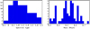 |
Fig. 1 Distribution of spectral types (left panel) and masses (right panel) for the HADES M dwarf sample. Negative indices denote spectral types earlier than M, where the value − 0.5 stands for K7.5. |
2 Stellar sample
Our stellar sample was observed in the framework of the HArps-N red Dwarf Exoplanet Survey (HADES; Affer et al. 2016; Perger et al. 2017) a collaborative effort between the Global Architecture of Planetary Systems project (GAPS, Covino et al. 2013), the Institut de Ciències de l’Espai (ICE/CSIC), and the Instituto de Astrofísica de Canarias (IAC). The sample amounts to 78 late K/early M dwarfs and covers an effective temperature range from 3400 to 3900 K, corresponding to spectral types from K7.5 to M4V (Fig. 1, left panel) and masses from about 0.3 to 0.75 M⊙ (Fig. 1, right panel). We group the stars in bins of 0.5 spectral subclasses, with K7.5 corresponding to −0.5, M0 to 0, and so on until M4, which is the last sub-type for which we have stars in our sample.
The stars were selected from the Palomar-Michigan State University (PMSU) catalogue (Reid et al. 1995), Lépine & Gaidos (2011) and are targets observed by the APACHE transit survey (Sozzetti et al. 2013) with a visible magnitude lower than 12. High-resolution échelle spectra of the stars were obtained at La Palma observatory (Canary Islands, Spain) during several observing runs between September 2012 and November 2017 using the HARPS-N instrument (Cosentino et al. 2012) at the Telescopio Nazionale Galileo (TNG). HARPS-N spectra cover the wavelength range 383–693 nm with a resolving power of R = 115 000 and all the spectra were automatically reduced using the Data Reduction Software (DRS, Lovis & Pepe 2007). Basic stellar parameters (effective temperature, spectral type, surface gravity, iron abundance, mass, radius, and luminosity) were computed and published by Maldonado et al. (2017) as part of the HADES collaboration using a methodology based on ratios of spectral features (Maldonado et al. 2015). The methodology consists of using ratios of pseudo-equivalent widths of spectral features as a temperature diagnostic. A list of calibrators was built for each of the basic stellar parameters considered (Teff, spectral type, and metallicity) and the derived temperatures and metallicities were used together with photometric estimates of mass, radius, and surface gravity (more details in Maldonado et al. 2015).
3 Rotation periods
The determination of the rotation periods (Prot) was done by analysing time series high-resolution spectroscopy of the Ca II H & K lines and Hα activity indicators and was published in Suárez Mascareño et al. (2018). The authors studied a fraction of our original M dwarf sample composed of 72 stars (out of a total of 78) providing 33 rotation periods measured from the spectral indicator modulation, and 34 periods derived from the Ca II H & K - rotational period relationship. The distribution of rotation periods is shown in Fig. 2. It can be seen that our Prot values coverthe range from 8 to 85 days. This interval exactly corresponds to a specific region where planets in the habitable zone around low-mass stars could be discovered. In other words, the period of planets in the habitable zone orbiting early M dwarfs coincides with the stellar rotation period (as shown in Fig. 1 from Newton et al. 2016).
The vast majority of our studied sample covers the stellar rotation period range from 15 to 60 days and mass range to 0.3 to 0.75 M⊙.
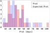 |
Fig. 2 Distribution of the rotation periods for the stars in our sample. The red area shows the measured rotation periods and the blue area corresponds to the derived rotation periods when a direct determination was not possible. |
4 Coronal activity
As said in previous sections, traditionally the most frequently investigated diagnostics of chromospheric activity are the Ca II H & K and the Balmer lines measured from optical spectra. In general, the Hα line has a complex structure, while Ca II H & K lines are difficult to measure in red stars. To measure a stellar activity diagnostic independently of the optical spectra, we decided to investigate the coronal activity indicator X-ray luminosity (Lx ); Lx is emitted from the upper atmosphere and can be easily determined for nearby M stars.
With the purpose of studying the coronal activity, we collected the information for our sample of 78 M dwarfs from the main X-ray missions, XMM-Newton, Chandra, and ROSAT (e.g. Truemper 1992; Voges et al. 1999) following this order of preference. Using The High Energy Astrophysics Science Archive Research Center (HEASARC)1 we find what X-ray mission observed our selected targets or if they were observed by more than one mission, in which case we followed the established preference. Even if ROSAT is older and less sensitive than the most recent X-ray observatories, it is still the main source of X-ray measurements since it covered all the sky. In particular, the catalogues that provided us X-ray information were the ROSAT Bright and Faint Source Catalogues (BSC and FSC; Voges et al. 1999), the second ROSAT All-Sky Survey Point Source Catalogue (2RXS; Boller et al. 2016), the third ROSAT Catalogue of Nearby Stars (CNS3; Hünsch et al. 1999), the XMM-Newton XAssist source list (XAssist; Ptak & Griffiths 2003), the XMM-Newton Slew Survey Full Source Catalogue, v2.0 (XMMSLEW; Saxton et al. 2008), and the Third XMM-Newton Serendipitous Source Catalogue (3XMM-DR7; Rosen et al. 2016).
For ROSAT detected sources, we need to apply a count-to-flux conversion factor (CF) because the X-ray emission is expressed by count rates (CRT) and hardness ratio (HR) quantities. The HR is defined through  , denoted by H and S the counts recorded in the soft (0.1–0.4 keV) and hard (0.5–2.0 keV) channels of the Position Sensitive Proportional Counters (PSPC) detector. In order to obtain the X-ray flux (fx ) from the PSPC detector, an appropriate conversion factor for a coronal spectral model must be computed (Schmitt et al. 1995):
 (1)
(1)
The conversion factor depends on the given spectral model and on the instrument, the details on this conversion procedure are given by Fleming et al. (1995). Clearly, the conversion needs some assumptions for the intrinsic source spectrum, but fortunately the conversion factor does not depend sensitively on the adopted coronal temperature, and the absorption due to the interstellar material can also be neglected because of the closeness of our stars. For the four cases with no HR in the database a HR value of − 0.4 is assumed, corresponding to a middle activity level star (Schmitt et al. 1995; Huensch et al. 1998; Sanz-Forcada et al. 2011) and then a fixed conversion factor value of 6.19 × 10⁻¹² erg cm−2 count−1 is used.
Combining the X-ray count rate with the conversion factor, the X-ray flux can be estimated as
 (2)
(2)
where the error on the observed flux is determined by the signal-to-noise ratio ( ):
):
 (3)
(3)
For XMM-Newton detected sources (G 243-30, GJ 412A, GJ 476, GJ 49, GJ 908, GJ 9440, NLTT 51676, and TYC 2703- 706-1) no conversion factor is needed because the X-ray emission is given directly on the observed flux with its correspondent error. Four of XMM-Newton detected sources (GJ 49, GJ 9440, GJ 908, and GJ 412A) were collected with the 3XMM-DR7 catalogue. We were then able to calculate for these targets the X-ray flux in the same energy band used by ROSAT using the Chandra Proposal Planning Toolkit PIMMS2. The X-ray flux was derived by assuming a plasma model (Astrophysical Plasma Emission Code, APEC), selecting the corresponding detector/filter used in the observation, and setting the appropriate input (0.2–12 keV, the total energy band used in the 3XMM-DR7 processing) and output energy band (0.1–2.4 keV, the total energy band in the ROSAT channels). For the rest of the sources detected by XMM-Newton (G 243-30, GJ 476, NLTT 51676, TYC 2703-706-1) the different XMM-Newton catalogues used (XMMSLEW and XAssist) did not allow us to use the previous approach with PIMMS due to a lack of information in the catalogue (e.g. detector/filter). Therefore, we provide directly the X-ray flux values reported in the corresponding catalogues (see XMM Science Survey Center memo SSC-LUX TN-0059 for a general description of the technique). We can estimate a systematic error introduced by the procedure described above of the order of 20–30%. In our analysis we did not use the XMM-Newton detected sources where it was not possible to convert the X-ray flux in the same energy band of ROSAT (G 243-30, GJ 476, NLTT 51676, and TYC 2703-706-1) because they had no information on the rotation period and there was no period derived from an activity–rotation relationship.
Once the X-ray flux value available for our targets is obtained, the X-ray luminosity can be derived by
 (4)
(4)
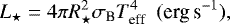
where fx corresponds to the X-ray observed flux and d is the distance to the star. Table 1 presents the 37 out of 78 stars with X-ray information collected for our M dwarf sample. The total uncertainties on the derived luminosities are calculated by error propagation. In Table 1 we also list the ratio Lx∕Lbol, where Lbol is the star bolometric luminosity, which is a measure of the coronal activity independent of the stellar size useful for a generalized analysis of the activity–rotation relation. The bolometric luminosity of the stars (L⋆ or Lbol ) was calculated following the Stefan–Boltzmann law
 (5)
(5)
where σB is the Stefan–Boltzmann constant (5.6704 × 10⁻⁵ erg cm−2 s−1 K−4), and R⋆ and Teff are the radius and effective temperature of the star, respectively, and were computed using the methodology based on ratios of spectral features described in Maldonado et al. (2015). The corresponding stellar parameters for our M dwarf sample were published in Maldonado et al. (2017).
4.1 Comparison with the nearby stellar population
In order to test how representative our M dwarf sample is of the solar neighbourhood, we compare its X-ray properties with a large sample of nearby M stars. The comparison sample is taken from the NEXXUS database (Schmitt & Liefke 2004), where only M dwarfs between M0 and M4.5 spectral types were selected (the same spectral type range for our sample). NEXXUS is a catalogue of all known stars within a distance of 25 pc to the Sun that are identified as X-ray and/or XUV-emitting stars from ROSAT data, based on positional coincidence. Figure 3 shows the cumulative distribution functions of log Lx for the NEXXUS M dwarfs and for our sample. The comparison clearly reveals that our sample shows higher levels of activity in X-ray emission with a log Lx median value about twice the median value of the nearby population. A Kolmogorov–Smirnov (K–S) test shows the significant difference between the two samples with a K–S statistic value D = 0.41 and p-value = 0.0002. We collected X-ray information close to 50% of the total sample. Therefore, as a rough approximation, we are studying the regime of moderately active M dwarfs and our search for exoplanets may be made more difficult by the presence of stellar activity.
Stars with derived X-ray emission.
4.2 Rotation period – activity relationship
In order to study the M star rotation–activity connection, we use the X-ray data collected in Sect. 4 and the rotation periods determined in the framework of the HADES collaboration and explained in Sect. 3. Merging the two quantities, our sample was reduced to 33 stars with both measurements. The final sample is given in Table 2 (a total of 19 measured Prot from the spectral indicators) and Table 3 (a total of 14 derived Prot from the Ca II H & K–Prot relationship).
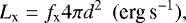
The mass range of our sample of M dwarfs (0.3–0.75 M⊙) is comparable with the M dwarf mass range of previous studies. In Fig. 4 we present an update of the activity–rotation relation of M dwarf stars using the X-ray data extracted from archives and the rotation periods by Suárez Mascareño et al. (2018), including stars with rotation periods derived from the activity–rotation relationship that are plotted as open circles (see below). We also indicate the relation derived by Pizzolato et al. (2003) and their sample of 21 stars for their lowest mass bin, M = 0.22–0.60 M⊙. It should benoted that the derived relation in the saturated regime by Pizzolato et al. (2003) is dominated by Prot values estimated from v sin i measurements (therefore only upper limit values for Prot) and only two stars are present in the non-saturated regime. On the other hand, most of our data fill the slow rotation area of low-mass stars covering the regime poorly populated in previous studies (e.g. Pizzolato et al. 2003; Stelzer et al. 2016).
In Fig. 4 (left panel), our data show a spread around the best-fit relation by Pizzolato et al. (2003). This spread is more evident in the right panel of Fig. 4 where log Lx∕Lbol is reported. It could be due to two possible reasons: (i) the mass range studied by Pizzolato et al. (2003; M = 0.22–0.60 M⊙ ) is too large and should be divided into subgroups; (ii) the derived rotational periods are too uncertain and their inclusion produces an artificially large spread.
On the one hand, we therefore excluded from our analysis the 14 derived Prot values (i.e. those derived from calcium measurements using a Ca II H & K–Prot relationship) maintaining only those with a direct measurement of the rotational period. Hereafter only periods measured from time series will be included in the analysis. On the other hand, we divided our sample into two Teff groups: 3400 ≤ Teff ≤ 3700 and 3700 ≤ Teff ≤ 3900 K (approximate mass range M = 0.3–0.47 M⊙ and M = 0.51–0.64 M⊙, respectively). This leaves us with a total of 19 M dwarfs in our sample, 11 stars in the 3400–3700 K range and 8 in the 3700–3900 K range. After discarding stars without a direct rotation period measurement, the correlations show a remarkably smaller dispersion (Fig. 5), indicating that we have identified the origin of the spread in Fig. 4.
Figure 5 shows the behaviour of M dwarfs in the non-saturated regime by dividing our stars into two Teff groups plotted with different colours. We do not have enough stars to determine here the saturated regime level (fast rotators) because almost all the stars in our sample are placed into the non-saturated regime. We assume the saturation level as described by Pizzolato et al. (2003). In a more recent work and using a larger sample, Stelzer et al. (2016) determine a higher saturation level than was found by Pizzolato et al. (2003). However, the sample in Stelzer et al. (2016) is taken from the Kepler Two-Wheel (K2) light curves and is likely biased towards bright X-ray M dwarfs, which can be translated into a higher value of the saturation level.
In order to obtain a new parametrization of the X-ray emission versus rotation relationship for M dwarfs in the non-saturated regime for the two bins of Teff, the data were fitted in each temperature bin with a fixed power-law exponent of − 2, leaving the intercept parameter free to vary. This value follows the well-studied and well-known relation (e.g. Pizzolato et al. 2003; Reiners et al. 2014) for the non-saturated regime, Lx ∝ P−2, indicating that the rotation period alone determines the X-ray emission. Power-law functions were fitted to the data
 (6)
(6)
where log F1 corresponds with the values of log Lx and log Lx∕Lbol, and a0 and a1 are the fit coefficients. In our case we set the value a1 fixed to − 2 and obtained the two best intercept parameters presented in Table 4.
The obtained best-fit relations between log Lx and Prot (Fig. 5, left panel) are very similar for the two Teff bins. We note the complementary behaviour of the log Lx∕Lbol versus Prot relation(Fig. 5, right panel) where the different loci occupied by the two Teff groups are more evident. This behaviour is coherent with the extension of Pizzolato et al. (2003) for more massive stars (F to late K stars) presented in Fig. 6, being our work an extension to the low mass regime that follows the observed trend for massive stars.
Using log Lx∕Lbol as an indicator, the relationship breaks down for low-mass stars that rotate very fast when X-ray luminosity reaches the approximately saturated value of log Lx∕Lbol ~−3 (e.g. Vilhu 1984; Pizzolato et al. 2003) independent of the stellar mass (except for the most massive bin). This saturation level is reached at rotation periods that increase towards less massive stars (increasing with decreasing the bolometric luminosity). On the contrary, if the log Lx indicator is considered, log Lx is a function of rotation period in the non-saturated regime and is independent from stellar mass.
This behaviour, across all spectral types, is clearly seen in Fig. 6 where we represent the collection of all best-fit relations found by Pizzolato et al. (2003) in all the mass ranges (F to late K stars) including the new relations found in this work in the non-saturated regime for early M dwarfs. In the left panel our best fitsare placed in the same range of non-saturated regime as all spectral types while in the right panel (log Lx∕Lbol vs. Prot) the new curve of the M dwarfs is on the right of the curves of more massive stars.
We have found a continuous shift of the log Lx∕Lbol versus Prot power-law towards longer Prot values extending the currently available sample of M dwarf stars to the non-saturated X-ray emission regime with respect to previous studies (e.g. Pizzolato et al. 2003; Stelzer et al. 2016; Wright et al. 2011). Consequently we are able to determine in a more accurate way than in previous works the value of rotation period at which the saturation occurs (Psat) for M dwarf stars. Assuming a defined saturated value for all mass ranges in log Lx∕Lbol as − 3.3 (except for the most massive bin that does not reach the same saturated value of the less massive bins; see right panel of Fig. 6) and knowing the mean value of log Lbol (for each temperature group) it is possible to estimate a better value for the rotation period  for each temperature bin in log Lx∕Lbol representation. Then we are able to obtain the correspondence of saturated rotation period value (
 ) in log Lx representation. The rotation period values derived from our sample at which X-ray emission reaches the saturation level and the values found in literature for early/middle M dwarfs are presented in Table 5.
In Fig. 7 we show the rotation period at which the saturation level is reached, Psat, both in Lx and Lx ∕Lbol representation, as a function of the different mass ranges used previously (Fig. 6). In both cases the overall behaviour of the Psat value along the different masses is to increase towards smaller stellar masses. Therefore, less massive targets will reach the saturated value at longer rotation periods.
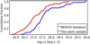 |
Fig. 3 Cumulative distribution function of log Lx. The red andblue lines correspond with the NEXXUS M dwarfs and this work sample, respectively. |
Stars with X-ray activity level and measured rotation periods.
Stars with X-ray activity level and derived rotation periods.
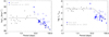 |
Fig. 4 Lx (left) and Lx∕Lbol (right) vs. rotation period. The black squares correspond to the stellar sample from Pizzolato et al. (2003) in the mass range 0.22 <M∕M⊙ < 0.60. The large blue dots correspond to the M dwarfs with periods measured from time series and used in the analysis. The open blue circles show the derived period from an activity–rotation relation (excluded from the analysis). The black dot-dashed line represents the broken power law obtained by the fitting procedure from Pizzolato et al. (2003) with Prot values estimated from vsini in saturated regime. |
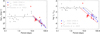 |
Fig. 5 Lx (left) and Lx∕Lbol (right) vs. rotation period for stars with direct rotation period determination. The black squares correspond to the stellar sample from Pizzolato et al. (2003) in the mass range 0.22 < M∕M⊙ < 0.60. The blue and red dots correspond to the M dwarfs from this work in the two different ranges of Teff indicated inthe legend. The black dot-dashed line represents the broken power law obtained by the fitting procedure from Pizzolato et al. (2003). The blue and red solid line represents our best fit for the 3400–3700 and 3700–3900 K Teff range, respectively. |
Coefficients of the activity–rotation relationships with slope set to −2.
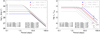 |
Fig. 6 All the best-fit relations between X-ray emission and rotational period for all the mass ranges (F to K stars) considered in Pizzolato et al. (2003) are presented as black lines. The blue and red solid line represents our best fit for the 3400–3700 and 3700–3900 K Teff range, respectively. |
X-ray saturated level for M dwarfs.
5 Summary and conclusions
The aim of this paper was to test whether the known relations in previous works between activity and stellar rotation for main-sequence FGK stars also hold for our sample of early M dwarfs. Computing the coronal activity indicator X-ray luminosity using the available data from ROSAT and XMM-Newton and using the rotation periods determined inside the HADES collaboration we were able to study the relation  that describes the non-saturated regime. We conclude that the relation is also valid for our targets extending the currently available sample of M dwarfs to the non-saturated X-ray emission regime. Our best-fit relations follow the observed trend for more massive stars in both representations, Lx and Lx∕Lbol versus Prot, which let us determine in a more accurate way than in previous works the calculated value at which the rotation period achieves saturation. This was possible by knowing the defined value of log Lx∕Lbol = −3.3 (Pizzolato et al. 2003) when the stars saturate and the mean value of log Lbol for each temperature group, and by considering the coefficients of the activity–rotation relationship estimated in this work.
We wanted to go one step further and study the age at which the saturation level is reached in M dwarfs. We used the angular momentum evolution models for 0.8 M⊙ and 0.3 M⊙ stars presented by Bouvier (2007) in Fig. 4 of that work. Following the models for slow and fast rotators shown by red solid lines, it is possible to make an estimation of the age at which the saturation level is reached. The rotational period is easily converted to angular velocity by Ω =2π∕Prot and scaled to the Sun (Ω⊙ = 2.87 × 10⁻⁶ s −1). On the one hand, for our sample in the mass range group ~0.3 M⊙ that reaches the saturation at  8 days, we can use the 0.3 M⊙ models to find that the saturation age is from 300 to 400 Myr. On the other hand, for the stars corresponding to those studied by Pizzolato et al. (2003), it is better to use the models computed for 0.8 M⊙ because of the different mass ranges, and the age at which they reach the saturation level could be defined before 300 Myr. The age range depends on the exact path followed by the star during its rotational evolution.
Finally, the importance of analysing the rotation period–activity relation using our sample of M dwarfs, and concluding that it is also valid for our targets, is that our data fill the slow rotation area. This area exactly corresponds with a specific region in which planets in habitable zone around low-mass stars could be discovered.
This confirms the big challenge that stellar activity poses for our radial velocity survey on discovering planets in early M dwarfs and our interest in a good understanding of stellar activity.
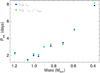 |
Fig. 7 Rotation period at which the saturation level (Psat) as a function of the stellar mass is reached. The blue and green dots correspond with the rotation period value at which the saturation occurs in Lx and Lx ∕Lbol representation, respectively. |
Acknowledgements
This work was supported by WOW from INAF through the Progetti Premiali funding scheme of the Italian Ministry of Education, University, and Research. This research has made use of data and/or software provided by the High Energy Astrophysics Science Archive Research Center (HEASARC), which is a service of the Astrophysics Science Division at NASA/GSFC and the High Energy Astrophysics Division of the Smithsonian Astrophysical Observatory. M.P. and I.R. acknowledge support from the Spanish Ministry of Economy and Competitiveness (MINECO) and the Fondo Europeo de Desarrollo Regional (FEDER) through grant ESP2016-80435-C2-1-R, as well as the support of the Generalitat de Catalunya/CERCA programme. J.I.G.H., R.R., and B.T.P. acknowledge financial support from the Spanish Ministry project MINECO AYA2017-86389-P. B.T.P. acknowledges Fundación La Caixa for the financial support received in the form of a Ph.D. contract. J.I.G.H. acknowledges financial support from the Spanish MINECO under the 2013 Ramón y Cajal program MINECO RYC-2013-14875. A.S.M. acknowledges financial support from the Swiss National Science Foundation (SNSF). G.S. acknowledges financial support from “Accordo ASI-INAF” No. 2013-016-R.0 July 9, 2013, and July 9, 2015. A.S.M. acknowledges financial support from the Swiss National Science Foundation (SNSF). M.Pi. gratefully acknowledges the support from the European Union Seventh Framework Programme (FP7/2007-2013) under Grant agreement no. 313014 (ETAEARTH).
References
- Affer, L., Micela, G., Damasso, M., et al. 2016, A&A, 593, A117 [NASA ADS] [CrossRef] [EDP Sciences] [Google Scholar]
- Astudillo-Defru, N., Delfosse, X., Bonfils, X., et al. 2017, A&A, 600, A13 [NASA ADS] [CrossRef] [EDP Sciences] [Google Scholar]
- Bean, J. L., Seifahrt, A., Hartman, H., et al. 2010, ApJ, 713, 410 [NASA ADS] [CrossRef] [Google Scholar]
- Boller, T., Freyberg, M. J., Trümper, J., et al. 2016, A&A, 588, A103 [NASA ADS] [CrossRef] [EDP Sciences] [Google Scholar]
- Bouvier, J. 2007, in Star-Disk Interaction in Young Stars, eds. J. Bouvier & I. Appenzeller, IAU Symp., 243, 231 [NASA ADS] [CrossRef] [Google Scholar]
- Browning, M. K., Basri, G., Marcy, G. W., West, A. A., & Zhang, J. 2010, AJ, 139, 504 [NASA ADS] [CrossRef] [Google Scholar]
- Cosentino, R., Lovis, C., Pepe, F., et al. 2012, in Ground-based and Airborne Instrumentation for Astronomy IV, Proc. SPIE, 8446, 84461V [Google Scholar]
- Covino, E., Esposito, M., Barbieri, M., et al. 2013, A&A, 554, A28 [NASA ADS] [CrossRef] [EDP Sciences] [Google Scholar]
- Delfosse, X., Forveille, T., Perrier, C., & Mayor, M. 1998, A&A, 331, 581 [NASA ADS] [Google Scholar]
- Dressing, C. D., & Charbonneau, D. 2013, ApJ, 767, 95 [NASA ADS] [CrossRef] [Google Scholar]
- Fleming, T. A., Molendi, S., Maccacaro, T., & Wolter, A. 1995, ApJS, 99, 701 [NASA ADS] [CrossRef] [Google Scholar]
- Henry, T. J., Jao, W.-C., Subasavage, J. P., et al. 2006, AJ, 132, 2360 [NASA ADS] [CrossRef] [Google Scholar]
- Howard, A. W., Marcy, G. W., Bryson, S. T., et al. 2012, ApJS, 201, 15 [NASA ADS] [CrossRef] [Google Scholar]
- Huensch, M., Schmitt, J. H. M. M., & Voges, W. 1998, A&AS, 132, 155 [NASA ADS] [CrossRef] [EDP Sciences] [Google Scholar]
- Hünsch, M., Schmitt, J. H. M. M., Sterzik, M. F., & Voges, W. 1999, A&AS, 135, 319 [NASA ADS] [CrossRef] [EDP Sciences] [Google Scholar]
- Kasting, J. F., Whitmire, D. P., & Reynolds, R. T. 1993, Icarus, 101, 108 [NASA ADS] [CrossRef] [PubMed] [Google Scholar]
- Kiraga, M., & Stepien, K. 2007, Acta Astron., 57, 149 [NASA ADS] [Google Scholar]
- Kosovichev, A. G., de Gouveia Dal Pino, E., & Yan, Y. 2013, in Solar and Astrophysical Dynamos and Magnetic Activity, IAU Symp., 294, 427 [NASA ADS] [Google Scholar]
- Lépine, S., & Gaidos, E. 2011, AJ, 142, 138 [NASA ADS] [CrossRef] [Google Scholar]
- Leto, G., Pagano, I., Buemi, C. S., & Rodono, M. 1997, A&A, 327, 1114 [NASA ADS] [Google Scholar]
- Lovis, C., & Pepe, F. 2007, A&A, 468, 1115 [NASA ADS] [CrossRef] [EDP Sciences] [Google Scholar]
- Maggio, A., Sciortino, S., Vaiana, G. S., et al. 1987, ApJ, 315, 687 [NASA ADS] [CrossRef] [Google Scholar]
- Maldonado, J., Affer, L., Micela, G., et al. 2015, A&A, 577, A132 [NASA ADS] [CrossRef] [EDP Sciences] [Google Scholar]
- Maldonado, J., Scandariato, G., Stelzer, B., et al. 2017, A&A, 598, A27 [NASA ADS] [CrossRef] [EDP Sciences] [Google Scholar]
- Matt, S. P., Brun, A. S., Baraffe, I., Bouvier, J., & Chabrier, G. 2015, ApJ, 799, L23 [NASA ADS] [CrossRef] [Google Scholar]
- Mohanty, S., & Basri, G. 2003, ApJ, 583, 451 [NASA ADS] [CrossRef] [Google Scholar]
- Newton, E. R., Irwin, J., Charbonneau, D., Berta-Thompson, Z. K., & Dittmann, J. A. 2016, ApJ, 821, L19 [NASA ADS] [CrossRef] [Google Scholar]
- Newton, E. R., Irwin, J., Charbonneau, D., et al. 2017, ApJ, 834, 85 [NASA ADS] [CrossRef] [Google Scholar]
- Noyes, R. W., Hartmann, L. W., Baliunas, S. L., Duncan, D. K., & Vaughan, A. H. 1984, ApJ, 279, 763 [NASA ADS] [CrossRef] [Google Scholar]
- Osten, R. A., Hawley, S. L., Allred, J. C., Johns-Krull, C. M., & Roark, C. 2005, ApJ, 621, 398 [NASA ADS] [CrossRef] [Google Scholar]
- Pallavicini, R., Golub, L., Rosner, R., et al. 1981, ApJ, 248, 279 [NASA ADS] [CrossRef] [Google Scholar]
- Perger, M., García-Piquer, A., Ribas, I., et al. 2017, A&A, 598, A26 [NASA ADS] [CrossRef] [EDP Sciences] [Google Scholar]
- Pizzolato, N., Maggio, A., Micela, G., Sciortino, S., & Ventura, P. 2003, A&A, 397, 147 [NASA ADS] [CrossRef] [EDP Sciences] [Google Scholar]
- Ptak, A., & Griffiths, R. 2003, in Astronomical Data Analysis Software and Systems XII, eds. H. E. Payne, R. I. Jedrzejewski, & R. N. Hook, in ASP Conf. Ser., 295, 465 [NASA ADS] [Google Scholar]
- Randich, S., Schmitt, J. H. M. M., Prosser, C. F., & Stauffer, J. R. 1996, A&A, 305, 785 [NASA ADS] [Google Scholar]
- Reid, I. N., Hawley, S. L., & Gizis, J. E. 1995, AJ, 110, 1838 [NASA ADS] [CrossRef] [Google Scholar]
- Reid, I. N., Gizis, J. E., & Hawley, S. L. 2002, AJ, 124, 2721 [NASA ADS] [CrossRef] [Google Scholar]
- Reiners, A., Joshi, N., & Goldman, B. 2012, AJ, 143, 93 [NASA ADS] [CrossRef] [Google Scholar]
- Reiners, A., Schüssler, M., & Passegger, V. M. 2014, ApJ, 794, 144 [NASA ADS] [CrossRef] [Google Scholar]
- Robinson, R. D., Cram, L. E., & Giampapa, M. S. 1990, ApJS, 74, 891 [NASA ADS] [CrossRef] [Google Scholar]
- Rosen, S. R., Webb, N. A., Watson, M. G., et al. 2016, A&A, 590, A1 [NASA ADS] [CrossRef] [EDP Sciences] [Google Scholar]
- Sanz-Forcada, J., Micela, G., Ribas, I., et al. 2011, A&A, 532, A6 [NASA ADS] [CrossRef] [EDP Sciences] [Google Scholar]
- Saxton, R. D., Read, A. M., Esquej, P., et al. 2008, A&A, 480, 611 [NASA ADS] [CrossRef] [EDP Sciences] [Google Scholar]
- Schmitt, J. H. M. M., & Liefke, C. 2004, A&A, 417, 651 [NASA ADS] [CrossRef] [EDP Sciences] [Google Scholar]
- Schmitt, J. H. M. M., Fleming, T. A., & Giampapa, M. S. 1995, ApJ, 450, 392 [NASA ADS] [CrossRef] [Google Scholar]
- Sozzetti, A., Bernagozzi, A., Bertolini, E., et al. 2013, Eur. Phys. J. Web Conf., 47, 03006 [CrossRef] [Google Scholar]
- Stassun, K. G., Hebb, L., Covey, K., et al. 2011, 16th Cambridge Workshop on Cool Stars, Stellar Systems, and the Sun, eds. C. Johns-Krull, M. K. Browning, & A. A. West, ASP Conf. Ser., 448, 505 [NASA ADS] [Google Scholar]
- Stelzer, B., Alcalá, J., Biazzo, K., et al. 2012, A&A, 537, A94 [NASA ADS] [CrossRef] [EDP Sciences] [Google Scholar]
- Stelzer, B., Marino, A., Micela, G., López-Santiago, J., & Liefke, C. 2013, MNRAS, 431, 2063 [NASA ADS] [CrossRef] [MathSciNet] [Google Scholar]
- Stelzer, B., Damasso, M., Scholz, A., & Matt, S. P. 2016, MNRAS, 463, 1844 [NASA ADS] [CrossRef] [Google Scholar]
- Strassmeier, K. G., Fekel, F. C., Bopp, B. W., Dempsey, R. C., & Henry, G. W. 1990, ApJS, 72, 191 [NASA ADS] [CrossRef] [Google Scholar]
- Suárez Mascareño, A., Rebolo, R., González Hernández, J. I., & Esposito, M. 2015, MNRAS, 452, 2745 [NASA ADS] [CrossRef] [Google Scholar]
- Suárez Mascareño, A., Rebolo, R., González Hernández, J. I., et al. 2018, A&A, 612, A89 [NASA ADS] [CrossRef] [EDP Sciences] [Google Scholar]
- Truemper, J. 1992, QJRAS, 33, 165 [NASA ADS] [Google Scholar]
- Vidotto, A. A., Jardine, M., Morin, J., et al. 2013, A&A, 557, A67 [NASA ADS] [CrossRef] [EDP Sciences] [Google Scholar]
- Vilhu, O. 1984, A&A, 133, 117 [NASA ADS] [Google Scholar]
- Voges, W., Aschenbach, B., Boller, T., et al. 1999, A&A, 349, 389 [NASA ADS] [Google Scholar]
- West, A. A., Weisenburger, K. L., Irwin, J., et al. 2015, ApJ, 812, 3 [NASA ADS] [CrossRef] [Google Scholar]
- Wright, N. J., Drake, J. J., Mamajek, E. E., & Henry, G. W. 2011, ApJ, 743, 48 [NASA ADS] [CrossRef] [Google Scholar]
- Wright, N. J., Newton, E. R., Williams, P. K. G., Drake, J. J., & Yadav, R. K. 2018, MNRAS, 479, 2351 [NASA ADS] [CrossRef] [Google Scholar]
All Tables
All Figures
|
Fig. 1 Distribution of spectral types (left panel) and masses (right panel) for the HADES M dwarf sample. Negative indices denote spectral types earlier than M, where the value − 0.5 stands for K7.5. |
| In the text | |
|
Fig. 2 Distribution of the rotation periods for the stars in our sample. The red area shows the measured rotation periods and the blue area corresponds to the derived rotation periods when a direct determination was not possible. |
| In the text | |
|
Fig. 3 Cumulative distribution function of log Lx. The red andblue lines correspond with the NEXXUS M dwarfs and this work sample, respectively. |
| In the text | |
|
Fig. 4 Lx (left) and Lx∕Lbol (right) vs. rotation period. The black squares correspond to the stellar sample from Pizzolato et al. (2003) in the mass range 0.22 <M∕M⊙ < 0.60. The large blue dots correspond to the M dwarfs with periods measured from time series and used in the analysis. The open blue circles show the derived period from an activity–rotation relation (excluded from the analysis). The black dot-dashed line represents the broken power law obtained by the fitting procedure from Pizzolato et al. (2003) with Prot values estimated from vsini in saturated regime. |
| In the text | |
|
Fig. 5 Lx (left) and Lx∕Lbol (right) vs. rotation period for stars with direct rotation period determination. The black squares correspond to the stellar sample from Pizzolato et al. (2003) in the mass range 0.22 < M∕M⊙ < 0.60. The blue and red dots correspond to the M dwarfs from this work in the two different ranges of Teff indicated inthe legend. The black dot-dashed line represents the broken power law obtained by the fitting procedure from Pizzolato et al. (2003). The blue and red solid line represents our best fit for the 3400–3700 and 3700–3900 K Teff range, respectively. |
| In the text | |
|
Fig. 6 All the best-fit relations between X-ray emission and rotational period for all the mass ranges (F to K stars) considered in Pizzolato et al. (2003) are presented as black lines. The blue and red solid line represents our best fit for the 3400–3700 and 3700–3900 K Teff range, respectively. |
| In the text | |
|
Fig. 7 Rotation period at which the saturation level (Psat) as a function of the stellar mass is reached. The blue and green dots correspond with the rotation period value at which the saturation occurs in Lx and Lx ∕Lbol representation, respectively. |
| In the text | |
Current usage metrics show cumulative count of Article Views (full-text article views including HTML views, PDF and ePub downloads, according to the available data) and Abstracts Views on Vision4Press platform.
Data correspond to usage on the plateform after 2015. The current usage metrics is available 48-96 hours after online publication and is updated daily on week days.
Initial download of the metrics may take a while.