| Issue |
A&A
Volume 624, April 2019
|
|
|---|---|---|
| Article Number | A6 | |
| Number of page(s) | 13 | |
| Section | Interstellar and circumstellar matter | |
| DOI | https://doi.org/10.1051/0004-6361/201834337 | |
| Published online | 29 March 2019 | |
Distances to molecular clouds at high galactic latitudes based on Gaia DR2
1
Purple Mountain Observatory,
Nanjing
210008,
PR China
2
Shanghai Astronomical Observatory, Chinese Academy of Sciences,
Shanghai
200030,
PR China
3
School of Astronomy and Space Science, University of Chinese Academy of Sciences,
19A Yuquanlu,
Beijing
100049, PR China
4
International Centre for Radio Astronomy Research, Curtin University,
GPO Box U1987,
Perth
WA
6845, Australia
5
Department of Physics and Astronomy and MQ Research Centre in Astronomy, Astrophysics and Astrophotonics, Macquarie University,
NSW
2109, Australia
Received:
28
September
2018
Accepted:
8
February
2019
Abstract
We report the distances of molecular clouds at high Galactic latitudes (|b| > 10°) derived from parallax and G-band extinction (AG) measurements in the second Gaia data release, Gaia DR2. Aided by Bayesian analyses, we determined distances by identifying the breakpoint in the extinction AG toward molecular clouds and using the extinction AG of Gaia stars around molecular clouds to confirm the breakpoint. We used nearby star-forming regions, such as Orion, Taurus, Cepheus, and Perseus, whose distances are well known to examine the reliability of our method. By comparing with previous results, we found that the molecular cloud distances derived from this method are reliable. The systematic error in the distances is approximately 5%. In total, 52 molecular clouds have well-determined distances, most of which are at high Galactic latitudes, and we provide reliable distances for 13 molecular clouds for the first time.
Key words: dust, extinction / ISM: clouds
e-mail: This email address is being protected from spambots. You need JavaScript enabled to view it.
© ESO 2019
1 Introduction
Determining the distances of molecular clouds, the birthplaces of stars, is usually difficult. Many distance measurement methods, such as the photometric parallax method and the period-luminosity relation, are not applicable to molecular clouds. However, the distance relates directly to many important properties of molecular clouds, especially the mass and size, making their physical states and relationships with Galactic spiral arms largely uncertain.
There are a few approaches to derive molecular cloud distances, but they usually either yield large uncertainties or are not applicable to diffuse and translucent molecular clouds at high Galactic latitudes. For instance, maser astrometry with multiple-epoch Very Long Baseline Interferometry (VLBI) measurements (Xu et al. 2009; Zhang et al. 2013; Ortiz-León et al. 2017a) cannot be performed toward molecular clouds that lack masers. Furthermore, kinematic distance estimates based on modeled rotation curves (Roman-Duval et al. 2009; Rice et al. 2016) suffer from large uncertainties and ambiguities.
Optical extinction provides another approach to determining the cloud distances. However, the optical extinction derived from counting stars toward molecular clouds (Bok 1937; Magnani & de Vries 1986) involves large uncertainties. A more straightforward but sophisticated way is to examine the variation in optical extinction with respect to distance along the line of sight (see Knude & Hog 1998). For example, using this method, Schlafly et al. (2014) provided a large distance catalog of 18 well-known star-forming regions, and 108 molecular clouds with high Galactic latitude were cataloged by Magnani et al. (1985, hereafter denoted MBM). They derived the distance and extinction for each star simultaneously from Pan-STARRS1 (Kaiser et al. 2010; Green et al. 2014) photometry and subsequently estimated the molecular cloud distances according to the breakpoint of the extinction. However, as Schlafly et al. (2014) have pointed out, their distances may have a ~10% systematic uncertainty.
The release of the second Gaia data (Gaia Collaboration 2016; Gaia Collaboration 2018), Gaia DR2, providing parallaxes for about 1.3 billion stars, a large proportion of which have G-band extinction (AG) measurements, has advanced this approach substantially. The correspondence between the extinction AG map (Arenou et al. 2018) and the distribution of molecular clouds (Dame et al. 2001) suggests that through AG, we may be capable of detecting molecular clouds. Although, as cautioned by Gaia Collaboration (2018), AG has large uncertainties, it is found to be reliable on average (see Andrae et al. 2018).
Gaia DR2 permits a more precise analysis of the extinction caused by molecular clouds than was previously possible and offers an independent means of examining the distance estimates of Schlafly et al. (2014). The rest of this paper is organized as follows. In Sects. 2 and 3, we introduce the method of reducing Gaia data and the process of deriving molecular cloud distances. We present the distance catalog in Sect. 4 and compare the results with previous studies in Sect. 5. The conclusions are summarized in Sect. 6.
2 Gaia DR2 and Planck 857 GHz data
We primarily investigated diffuse molecular clouds at |b| > 10°, which are less likely to be contaminated by other molecular clouds that are either adjacent or overlap along the line of sight. Despite being located at high Galactic latitudes, they are usually at a distance closer than 1 kpc from the Sun and are still located in the Galactic plane (Magnani et al. 1996; Schlafly et al. 2014). They tend to occupy large areas on thesky, making them able to optically extinct a large number of stars. Consequently, the extinction AG imposed on stars behind molecular clouds can be investigated statistically.
We selected Gaia DR2 stars according to their parallaxes and extinction AG. First, we removed stars with parallaxes <0.5 mas, corresponding to an upper distance threshold of 2 kpc. Molecular clouds at high Galactic latitudes are usually near the Sun (<1 kpc), and a 2 kpc cutoff suffices for our study. If the relative errors of stellar parallaxes were to exceed 20%, the corresponding distances would differ from the reciprocal of their parallaxes by a large amount (Bailer-Jones 2015), and consequently, we only kept stars whose relative parallax errors are smaller than 20%. For AG, we required AG > 0, which rejected 13 stars. In total, 30 259 242 Gaia stars meet these criteria.
The extinction AG error of a single star, ΔAG, is estimated with
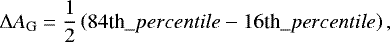 (1)
(1)
where 84th_percentile and 16th_percentile are provided in Gaia DR2. To derive the distance and its standard deviation, we drew 10 000 samples from the Gaussian distribution  , where ϖ and Δϖ are the parallax and its error in Gaia DR2, and the mean and standard deviation of the distance corresponds to the mean and standard deviation of the reciprocal of the 10 000 samples, respectively.
We used Planck 857 GHz images (Planck Collaboration I 2014) to trace the molecular clouds rather than IRAS 100 μm and CO spectral lines. Although the IRAS 100 μm images (Schlegel et al. 1998; Miville-Deschênes & Lagache 2005) have a similar spatial resolution (5′) as the Planck 857 GHz survey, the sensitivity of the Planck 857 GHz survey is higher, and consequently, the Planck 857 GHz survey classifies Gaia stars more accurately and produces slightly better results, details of which are discussed in Sect. 4.1. Planck 857 GHz data are more complete than CO survey data (Dame et al. 2001) at high Galactic latitudes, and although Planck 857 GHz emission cannot distinguish molecular cloud components that overlap each other along the line of sight, this situation is not severe at high Galactic latitudes, and usually only one nearby molecular cloud component is present in one direction. The Planck 857 GHz images were only used to classify Gaia DR2 stars, not to build dust models.
3 Method
In this section we describe the method of deriving molecular cloud distances with the Gaia DR2 and Planck 857 GHz data. Principally, molecular clouds increase the extinction AG of all stars behind them, thus producing breakpoints in AG along the line of sight. Consequently, identifying the breakpoints in AG is the essentialpoint in our method.
First, we collected two classes of Gaia stars, on- and off-cloud stars, based on Planck 857 GHz emission. On-cloud stars, showing breakpoints in AG, are the Gaia stars toward molecular clouds. We define as “off-cloud stars” Gaia stars around molecular clouds, and because they are not affected by molecular clouds, off-cloud stars have no breakpoints in AG. Practically, the breakpoints were determined with on-cloud stars alone, while off-cloud stars were used to confirm the breakpoints by eye. The schematic diagram of Fig. 1 depicts the extinction AG feature of on- (green) and off-cloud (blue) stars.
In the second step, the distances were determined using Bayesian inference with on-cloud stars and were subsequently confirmed with off-cloud stars by eye. We use two molecular clouds, Taurus (Pineda et al. 2010; Ward-Thompson et al. 2016) and Gemini (Li et al. 2015), to illustrate the process of determining distances.
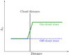 |
Fig. 1 Extinction AG of on- (green) and off-cloud (blue) stars. The vertical black line marks the distance of the molecular cloud. |
3.1 On- and off-cloud stars
The on- andoff-cloud stars were classified according to Planck 857 GHz intensity thresholds. The on-cloud stars are those whose Planck 857 GHz emission is stronger than an intensity threshold (the signal level), while toward off-cloud stars, the Planck 857 GHz emission is fainter than a lower threshold (the noise level). We determined the two thresholds through fitting a mixed distribution combining two functions, Gaussian and exponential, as described below.
First, we manually drew a box region for each molecular cloud, and only Gaia stars in this box region were considered. This region contained at least part of the molecular cloud and incorporated an additional nearby region. This additional region, where the Planck 857 GHz emission was significantly lower than the molecular cloud region, contained off-cloud stars. Thesebox regions are not necessarily the same as the traditional boundaries of molecular clouds, that is, they may be larger or smaller than the entire molecular clouds as long as these regions contain sufficient Gaia stars.
Second, we assigned each Gaia star a Planck 857 GHz emission value according to the Planck 857 GHz data. As the histograms demonstrate in Fig. 2, the Planck 857 GHz emission roughly contains two components: (1) a background noise that has an approximately Gaussian distribution in intensity, and (2) the molecular cloud emission that resembles an exponential distribution.
We used four parameters to model this mixed distribution: the mean (μ) and the standard deviation (σ) of the Gaussian part, a switch point (SP), and the rate(λ) of the exponential distribution. The cumulative distribution function (CDF) of the mixed distribution (the likelihood) is
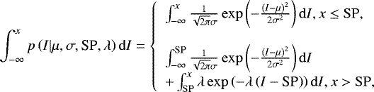 (2)
(2)
where I is the observed Planck 857 GHz intensity.
The four parameters were estimated by maximizing this likelihood, and the noise and signal level were subsequently determined according to the two distributions. As demonstrated in Fig. 2, we used a noise level of Gaussian mean μ, and a signal level of exponential median 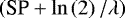 .
.
There is a trade-off in the choice of the signal level. Lower signal levels keep more stars, which is good for a statistical analysis, but involve many stars with low extinction AG, which smears the breakpoints. Higher signal levels make the breakpoints evident, but fewer stars remain. The signal level, the median value of the exponential component, is a compromise choice. However, in Sect. 4.2, we show that as long as the breakpoints are detected, the derived distances are insensitive to the choice of signal levels.
The signal and noise levels classify on- and off-cloud stars, respectively. Although only on-cloud stars were employed to calculate distances, the off-cloud stars are useful as a reference to confirm the breakpoints.
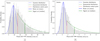 |
Fig. 2 Determining the noise and signal levels to classify on- and off-cloud stars for the Taurus (panel a) and Gemini (panel b) molecular clouds. The blue and green dashed lines represent the Gaussian and exponential distribution, respectively, and the dashed vertical red lines mark the switch point between the two distributions. We use the Gaussian mean (the solid vertical blue lines) for the noise cutoff level and the exponential median (the solid vertical green lines) for the signal cutoff level. |
3.2 Estimating the distance
With the extinction AG and the corresponding distances of on- and off-cloud stars, we are now in the position to calculate the distance of molecular clouds. We built a Bayesian model to estimate the distance with on-cloud stars and solved for the parameters in the model with Markov chain MonteCarlo (MCMC) sampling. We emphasize that off-cloud stars were not involved in the model but were only used to confirm the breakpoint by eye.
The extinction AG of on-cloud stars includes three components: (1) the foreground AG, (2) the background AG, and (3) the transition values. When passing through a molecular cloud along the line of sight, the extinction AG gradually increases from the foreground AG (which is usually 0 mag) level to the background AG level. Here, we ignored the third component and focused on the average distance in our model. Because the minimum ( ) and maximum (
 ) values of the extinction AG are 0 and 3.609 mag, respectively, we followed the procedure of Andrae et al. (2018) using a truncated Gaussian distribution to model the on-cloud star extinction AG.
Our model involves four parameters, the cloud distance (D), the extinction AG dispersion (σ1) of foreground stars, and the extinction AG (μ2) and its dispersion (σ2) of background stars. We found that the extinction AG of foreground stars (μ1) is precisely zero, but for only four molecular clouds, therefore we used μ1 = 0 in most cases. Thesefour molecular clouds have additional small molecular cloud components in front of them, therefore they treated them separately. We used a lower distance cutoff to remove the foreground stars of the small molecular cloud components, and their μ1 were also modeled, which means that we used five parameters in total for them.
With these four parameters and a list of distances di with standard deviations Δdi, which were calculated with the reciprocal of 10 000 parallax samples (see Sect. 2), and extinction AG i (with standard deviations ΔAGi), we derive an appropriate likelihood below. This approach requires no binning, and the binned extinction AG and distances were only used for visual confirmation.
We calculated the likelihood of each star on the condition that it was in front of or behind the molecular cloud. Denoting the CDF of the standard normal distribution as
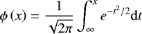 (3)
(3)
and given D, the probability for a star to be in front of the molecular cloud is
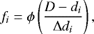 (4)
(4)
while the probability to be located behind the molecular cloud is 1 − fi.
The form of a truncated Gaussian distribution (Andrae et al. 2018), with mean μ and standard deviation σ, is
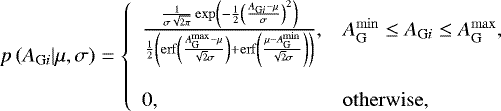 (5)
(5)
where
 (6)
(6)
In order to consider the measure error of the extinction AG, we convolved the standard deviation of the extinction AG, ΔAG i, with σ1 and σ2. Consequently, the likelihood of foreground stars is
 (7)
(7)
Similarly, the likelihood of background stars is
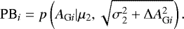 (8)
(8)
Consequently, the likelihood of a star is
 (9)
(9)
The total likelihood is the product of the likelihoods over all the stars, and we solved this model with MCMC sampling. In order to obtain a high sampling rate, we may need to set smart priors. The prior distribution of D was assumed to be uniform, so that the model can uniformly search the switch point, that is, the breakpoint of AG, along the line of sight. Denoting the minimum and maximum of di as Dmin and Dmax, the prior of D is  , where
  represents the uniform distribution and the 50 pc was set to avoid touching the edge. In practice, instead of sampling σ1 and σ2, we sampled their reciprocal, denoted as Iσ1 and Iσ2. The prior distributions of Iσ1, μ2, and I σ2 were assumed to be exponential, and here, we used a form of
  for the exponential distribution, where β is the mean. We summarize the priors as
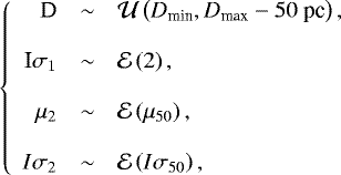 (10)
(10)
where  and
and  represent the uniform and exponential distributions, respectively, μ50 and Iσ50 are the mean and reciprocal standard deviation of AG of stars with distances
 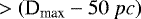 , and the initial guess of 2 mag−1 for I σ1 was derivedfrom the reciprocal of 0.45 mag, which is the typical extinction AG standard deviation of clustering stars derived by Andrae et al. (2018).
In order to decrease the autocorrelation time of the MCMC samples, we thinned the samples. Because the acceptance rate is about 25%, we thinned the samples by a factor of 15, considering only every 15th step in each chain, and the autocorrelation time is short (about 4) after thinning. We calculated eight independent chains, and each chain had 1000 thinned samples (with an additional 50 for burn-in, which means that the first 50 thinned samples were removed), that is, 8000 thinned posterior samples for each parameter. In order to increase the sampling speed, we used the Gibbs sampler (Geman & Geman 1984): we changed one parameter at a time and used the Metropolis–Hastings algorithm (Metropolis et al. 1953; Hastings 1970) for each time until all four parameters had obtained the next values. The state transition functions of the parameters are all Gaussian, whose standard deviations are 50 pc for D, 0.3 mag for μ2, and 0.3 mag−1 for Iσ1 and Iσ2.
We investigated the convergence of each chain with the Gelman–Rubin diagnostic (Gelman & Rubin 1992). The potential scale reduction factor (PSRF),  , is smaller than 1.01 for all molecular clouds except for Taurus (whose
  is about 6), which has two close components. Consequently, the MCMC chains have converged except for Taurus.
In order to verify the MCMC results, we compared the Gibbs sampler with the affine-invariant ensemble sampler (Goodman & Weare 2010) implemented by the Python MCMC module EMCEE (Foreman-Mackey et al. 2013). The EMCEE package usually produces many outliers, but when it occasionally generates less outliers, it gave the same results with the Gibbs sampler.
In order to balance the star numbers of the two truncated Gaussian components in Eq. (5) and to avoid the interference of farther molecular clouds along the line of sight, we set a distance cutoff for each molecular cloud. Because we need to know the distance before setting the distance cutoff, this is a recursive process. Usually, a distance cutoff of 1000 pc is sufficient, and we adjusted this cutoff for far or near molecular clouds when necessary. Close molecular clouds usually have too few foreground stars compared to background stars, and a small fluctuation of AG in the background stars would cause their distances to be incorrectly recognized.
A lower cutoff for foreground stars was not necessary except for four molecular clouds, which are the far component of Cepheus, Mon R2, Polaris, and Rosette. In oder to remove the effect of foreground components, we removed on-cloud stars that were nearer than 400, 500, 325, and 1000 pc to them, and the corresponding μ1 were estimated to be 0.683, 0.499, 0.295, and 0.839 mag, respectively. Because we had five parameters to model, we calculated ten chains for these four molecular clouds, that is, 10 000 thinned samples for each of them.
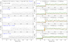 |
Fig. 3 Test of the model for calculating molecular cloud distances with simulated on-cloud stars. The simulated molecular cloud is assumed to be located at a distance of 300 pc. The reference values of parameters are displayed in the top left panel, and we change one parameter at any one time to see the variation in distance. Left column: simulated raw data. Right column: corresponding binned data and derived distance results with the model. The raw extinction AG and distances are averaged every 5 pc, weighted by their errors. Only raw data are used in the distance estimation, while the binned data are only used to confirm the results by eye. |
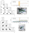 |
Fig. 4 Distance of the Taurus (panel a) and Gemini (panel b) molecular clouds. In the panels at the bottom right, showing the Planck 857 GHz images, purple circles mark the position of molecular clouds, while the blue and green contours correspond to the noise and signal thresholds in Fig. 2, respectively. Top right panel: green and blue points present on- and off-cloud stars (binned every 5 pc), respectively. The dashed red lines are the modeled extinction AG. The distances were derived with raw on-cloud Gaia DR2 stars, which are represented with gray points. The black vertical lines indicate the distance (D) estimated with Bayesian analyses and MCMC sampling, and the shadow areas depict the 95% HPD distance range. The corner plots of the MCMC samples are displayed on the left. The mean and 95% HPD of the samples are shown with solid and dashed vertical lines, respectively, and the systematic uncertainty is not included. The Taurus molecular cloud may contain two components. |
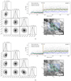 |
Fig. 5 Distances of molecular cloud HSVMT 5 produced with Planck 857 GHz (panel a) and IRAS 100 μm (panel b). See the caption of Fig. 4 for other details. |
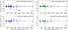 |
Fig. 6 Distance discrepancies and errors with altered parameters. The effect of molecular cloud region boxes is shown in panels a and b, and the signal levels are plotted in panels c and d. Only one molecular cloud, Gemini, shows large discrepancies (with magnitudes >40 pc), which is in case of panel a. |
3.3 Testing the model
We tested this model of calculating molecular cloud distances with simulated data before we applied it to Gaia DR2 stars. The simulated molecular cloud is at a distance of D = 300 pc, and the extinction of its foreground star is 0 mag, that is, μ1 = 0. The dispersions of the foreground and background stars AG are 0.3 and 0.6 mag, respectively, that is, σ1 = 0.3 mag and σ2 = 0.6 mag. We added scatter AG errors of 20–50% on the extinction AG, and stars whose extinction AG < 0 or > 3.609 mag were removed.
We changed four parameters, the extinction of the background star μ2, the number of stars per pc, the relative parallax errors, and the distance cutoff, to determine the variation in the resulting distances. As demonstrated in Fig. 3, our model detected the distances successfully in all cases. Unsurprisingly, smaller jumps in AG, fewer Gaia DR2 star samples, and larger parallax errors would cause larger distance errors, while the distance cutoff has no effect in the distance determination. Remarkably, although the distance errors became larger, the distance was still consistently recognized.
In Gaia DR2, the errors on distances are usually better than 10% for stars nearer than 1 kpc. Therefore, the two most important factors that may affect our results are the number of on-cloud stars and the magnitude of AG caused by molecular clouds.
3.4 Distance of the Taurus and Gemini molecular clouds
We applied our model to the Taurus and Gemini molecular clouds. The corner plots of the four parameters, D, σ1, μ2, and σ2, are displayed in Fig. 4, together with their means and 95% highest posterior densities (HPDs). In the bottom right panel, the dashed blue boxes of (a) and (b) are the manually chosen cloud regions (see Sect. 3.1), which contain molecular clouds and additional noise regions. The blue and green contours represent the noise and signal thresholds, respectively, which were determined in Sect. 3.1 (see Fig. 2). In the top right panel, we display the distances and on- and off-clouds stars with green and blue points, respectively. The derived distances to the Taurus and Gemini molecular clouds are  and
and  pc, respectively.
Interestingly, the Taurus molecular cloud seems to have two components. Farther away than 130 pc, many stars still have low extinction AG until about 150 pc. The Taurus distance given by Torres et al. (2009) is 161.2±0.9 pc, which may be corresponding to this component.
4 Molecular cloud distances
4.1 Planck 857 GHz versus IRAS 100 μm data
We demonstrate that Planck 857 GHz data trace dust better than IRAS 100 μm, or at least that these data better suited to our method. As an example, we show the distances of the molecular cloud HSVMT 5 produced with Planck 857 GHz and IRAS 100 μm in Fig. 5.
The distance estimated with Planck 857 GHz is  pc, and
  pc for IRAS 100 μm. As indicatedin Fig. 5, the average extinction of on-cloud stars classified with Planck 857 GHz is higher than that with IRAS 100 μm, suggesting that the on-cloud stars identified with Planck 857 GHz are less strongly contaminated by other Gaia stars that have low extinction AG. Consequently, the extinction values, AG, of the background stars are better separated from the foreground stars with Planck 857 GHz emission.
Comparison with VLBI distance measurements.
4.2 Effect of the parameter choice
In this subsection, we examine the reliability of our method and its dependence on parameters. In our method, we primarily involve two subjective parameters: the manually chosen molecular cloud region, and the signal level cutoff in the Planck 857 GHz intensity. In total, we found that 52 molecular clouds have well-determined distances with the chosen molecular cloud regions and signal levels.
In order to determine the influence of the two parameters, we shifted them one at a time and compared the distance variations. In Fig. 6 we display the distance discrepancies and uncertainties after altering parameters. To reveal the effect of the molecular cloud region box, we shifted the molecular cloud region box along l to the left and right by 10% of the box size in l, while the signal levels were altered by ±20%. The distances show slight fluctuations in the molecular clouds, while their uncertainties widely agree with the distances calculated with the chosen parameters. Clearly, large distance discrepancies usually yield large uncertainties, and no evident systematic deviations are present. Only Gemini shows large distance deviations (with magnitudes >40 pc) in case (a), confirming our claim that correct recolonization of breakpoints guarantees comparable distances.
Consequently, our distance estimation is robust and only weakly dependent on the choice of region boxes and signal levels in a reasonable range. In addition, in order to ensure that the breakpoints are genuine, it is necessary to confirm the breakpoints with off-cloud stars.
4.3 Distance catalog
With the method described in Sect. 3, we calculated distances for many molecular clouds at high Galactic latitude, most of which have been cataloged by Magnani et al. (1985, 1996) and Schlafly et al. (2014). In these three catalogs, many molecular clouds belong to the same molecular could complexes or filaments, and we only give one distance for each complex or filament because of the large dispersion in AG and because Gaia stars are not suitable for small subregions.
We have reproduced the distances of many star-forming regions, whose distances are well determined with VLBI measurements, such as Orion (Kounkel et al. 2017), Mon R2 (Dzib et al. 2016), Ophiuchus (Ortiz-León et al. 2017b), and Perseus (Ortiz-León et al. 2018). In Table 1 we compare our results with VLBI-measured distances. Considering the distance errors and dispersions, the molecular cloud distance given by Gaia DR2 agrees quite well with VLBI measurements. We suggest that VLBI and Gaia DR2 may see different components of the molecular clouds, and the slight discrepancies may be due to the structure of the molecular clouds.
We summarize the distances in Table A.1, listing 52 molecular clouds whose distances are well determined, that is, whose breakpoints are evident. The distances for many molecular clouds cannot be determined because (1) they are not well defined in Planck 857 GHz, (2) their optical depths are too low, or (3) their covering areas are too small. In the penultimate column, we indicate the molecular clouds whose distances are not provided by Schlafly et al. (2014) or were measured using VLBI with “Y”. There are 13 such clouds in total.
The distance figures of all molecular clouds are provided on Harvard Dataverse1.
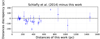 |
Fig. 7 Comparison of distances in our work with those from Schlafly et al. (2014). |
4.4 Systematic error
In this section, we estimate the systematic error in the distances. First, as suggested by the test results (see Fig. 3), the distances show a systematic error of 1–10%. In the testing data, we simulated parallax errors of 10–20% and within 1 kpc from the Sun, but the uncertainties of Gaia DR2 parallaxes are smaller than 10%. Therefore, the true systematic error is likely to be smaller.
Second, as shown in Fig. 6, the root mean squares (RMS) of the relative distance deviations in the four cases are 3% (a), 2% (b), 1% (c), and 2% (d), respectively. This suggests a systematic error of about 3% that is caused by subjective choices.
Third, if the VLBI results (see Table 1) are the true distances, our distances show a systematic error of ≤6%. However, VLBI usually measures the parallax of one single star, which may deviate from the main part of the molecular clouds.
Fourth, Lindegren et al. (2018) reported that the Gaia DR2 parallaxes have a systematic error of approximately 0.1 mas. Considering a molecular cloud at a distance of 500 pc (2 mas), this systematic parallax error causes a systematic error of about 5% in the distance.
Consequently, we estimate that the systematic distance error is about 5%. It might be slightly larger for distant molecular clouds.
5 Discussion
5.1 Comparison with previous results
In Fig. 7 we draw the distances derived from Gaia DR2 against those provided by Schlafly et al. (2014). We averaged the distances weighted by the square inverse of their errors when multiple distances (corresponding to the same molecular cloud) are provided by Schlafly et al. (2014). The distances provided by Schlafly et al. (2014) display a slight systematic shift, ~24 pc, toward the farther distances. In terms of relative errors, the systematic shift is, after removing one outliers (>70%), about 13%.
This systematic shift was predicted by Schlafly et al. (2014). They attributed the systematic errors to stellar models, dust models, and the reddening law. However, in addition to these, we found that the molecular regions used by Schlafly et al. (2014) are much smaller than the regions in our work, which means that their results may only represent the distances of molecular clouds in these small regions and are less affected by the thickness of the molecular clouds along the line of sight. Alternatively, nearer clouds are brighter and easily chosen, which could cause the distances given by Schlafly et al. (2014) to be systematically smaller.
However, the Gaia DR2 data may also contribute to this systematic error. The ~0.1 mas systematic parallax error in Gaia DR2 (Lindegren et al. 2018) may be one of the causes of the systematic distance discrepancy. At a typical distance of 500 pc, 0.1 mas error corresponds to ~25 pc shift, which can explain this systematic shift. Furthermore, the extinction AG, which has large uncertainties, may contain unknown systematic errors.
One means of examining the discrepancy is to compare the distance modulus in Schlafly et al. (2014) with the Gaia DR2 parallaxes. However, this is beyond the scope of this work, and alternatively, in Fig. 8, we display the distances of MBM11 and MBM7, which show large distance discrepancies. As shown in Fig. 8, the distances of MBM11 and MBM7 are  and
and  pc, respectively.However, in the distance catalog of Schlafly et al. (2014), the distance of the MBM11 molecular cloud is approximately 206±23 pc, which isthe average distance of MBM11, 12, 13, and 14, while the distance of MBM7 is
  pc. Based on Gaia DR2, the distances of these two molecular clouds, particularly MBM11, are well determined.
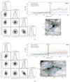 |
Fig. 8 Distance of MBM11 (panel a) and MBM7 (panel b). These two molecular clouds show large distance discrepancies with that provided by Schlafly et al. (2014). See the caption of Fig. 4 for other details. |
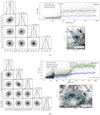 |
Fig. 9 Distances of near (panel a) and far (panel b) components in the Cepheus molecular cloud. See the caption of Fig. 4 for other details. |
5.2 Individual molecular cloud distances
In this subsection, we discuss the distances of several individual molecular clouds. Schlafly et al. (2014) obtained a distance of about 350 pc for the Ursa Major molecular clouds, which is much farther than previous studies, ~110 pc (Penprase 1993). Using Gaia DR2 data, we have derived a distance of  for the Ursa Major molecular clouds, which is close to the distance given by Schlafly et al. (2014).
Li et al. (2015) performed a survey of two CO isotopologue lines toward the same Gemini region as shown in Fig. 4. They used a distance of 400 pc, but Gaia DR2 clearly shows that its distance is about 725 pc. The masses and sizes of Gemini molecular cores calculated by Li et al. (2015) should be revised accordingly.
Cepheus (Grenier et al. 1989; Yonekura et al. 1997; Kirk et al. 2009) is an interesting region. As shown in Fig. 9, there are two obvious components along the line of sight. The distance of the nearer component is  pc, and the distance of the farther is
  pc. According to the CO observations of Grenier et al. (1989), the radial velocity range of the far component is about −12 km s−1, while the nearer component has a velocity of about 0 km s−1. The distances of the two components derived by Grenier et al. (1989) are ~300 and 800 pc, respectively, which are consistent with our results.
6 Summary
Using the parallaxes and extinction AG provided by Gaia DR2, we derived the distances for 52 molecular clouds, most of which are at high Galactic latitudes, that is, |b| > 10°. The systematic error of the distances is about 5%, and we determined reliable distances for 13 molecular clouds for the first time. In addition, wehave confirmed the distances of many star-forming regions, such as Orion, Taurus, Cepheus, and Mon R2.
We used Planck 857 GHz data rather than CO data to trace molecular clouds because CO observations are incomplete at high Galactic latitudes. However, at low Galactic latitudes (|b| ≤ 10°), multiwavelength observations with high spatial resolutions would classify on- and off-cloud stars more accurately.
Gaia DR2 has enabled us to determine the distances of many nearby molecular clouds efficiently. Although the large errors of extinction AG in Gaia DR2 prevent us from examining distant (>2 kpc) molecular clouds, with the improved qualities of distances and extinction AG in future Gaia data releases, we would be able to obtain the distances of many more molecular clouds.
Acknowledgements
We thank Mario G. Lattanzi for his valuable comments and careful proofreading. We are grateful to an anonymous referee for their constructive comments, particularly on the distance likelihood and the MCMC method. This work was sponsored by the Ministry of Science and Technology (MOST) Grant No. 2017YFA0402701, the 100 Talents Project of the Chinese Academy of Sciences (CAS), the National Science Foundation of China under Grand NO. 11673051 and 11873019, the CAS Grand No. QYZDJ-SSW-SLH047, and the Key Laboratory for Radio Astronomy, CAS.
Appendix A Additional table
Molecular cloud distances.
References
- Andrae, R., Fouesneau, M., Creevey, O., et al. 2018, A&A, 616, A8 [NASA ADS] [CrossRef] [EDP Sciences] [Google Scholar]
- Arenou, F., Luri, X., Babusiaux, C., et al. 2018, A&A, 616, A17 [Google Scholar]
- Bailer-Jones, C. A. L. 2015, PASP, 127, 994 [NASA ADS] [CrossRef] [Google Scholar]
- Bok, B. J. 1937, The Distribution of the Stars in Space (Chicago: University of Chicago Press) [Google Scholar]
- Dame, T. M., Hartmann, D., & Thaddeus, P. 2001, ApJ, 547, 792 [NASA ADS] [CrossRef] [Google Scholar]
- Dzib, S. A., Ortiz-León, G. N., Loinard, L., et al. 2016, ApJ, 826, 201 [NASA ADS] [CrossRef] [Google Scholar]
- Foreman-Mackey, D., Hogg, D. W., Lang, D., & Goodman, J. 2013, PASP, 125, 306 [CrossRef] [Google Scholar]
- Gaia Collaboration (Prusti, T., et al.) 2016, A&A, 595, A1 [NASA ADS] [CrossRef] [EDP Sciences] [Google Scholar]
- Gaia Collaboration (Brown, A. G. A., et al.) 2018, A&A, 616, A1 [NASA ADS] [CrossRef] [EDP Sciences] [Google Scholar]
- Gelman, A., & Rubin, D. B. 1992, Stat. Sci., 7, 457 [Google Scholar]
- Geman, S., & Geman, D. 1984, IEEE Trans. Pattern Anal. Mach. Intell., 6, 721 [CrossRef] [PubMed] [Google Scholar]
- Goodman, J., & Weare, J. 2010, Commun. Appl. Math. Comput. Sci., 5, 65 [Google Scholar]
- Green, G. M., Schlafly, E. F., Finkbeiner, D. P., et al. 2014, ApJ, 783, 114 [NASA ADS] [CrossRef] [Google Scholar]
- Grenier, I. A., Lebrun, F., Arnaud, M., Dame, T. M., & Thaddeus, P. 1989, ApJ, 347, 231 [NASA ADS] [CrossRef] [Google Scholar]
- Hastings, W. K. 1970, Biometrika, 57, 97 [Google Scholar]
- Kaiser, N., Burgett, W., Chambers, K., et al. 2010, Proc. SPIE, 7733, 77330E [Google Scholar]
- Kirk, J. M., Ward-Thompson, D., Di Francesco, J., et al. 2009, ApJS, 185, 198 [NASA ADS] [CrossRef] [Google Scholar]
- Knude, J., & Hog, E. 1998, A&A, 338, 897 [NASA ADS] [Google Scholar]
- Kounkel, M., Hartmann, L., Loinard, L., et al. 2017, ApJ, 834, 142 [NASA ADS] [CrossRef] [Google Scholar]
- Li, Y., Xu, Y., Yang, J., et al. 2015, AJ, 150, 60 [NASA ADS] [CrossRef] [Google Scholar]
- Lindegren, L., Hernández, J., Bombrun, A., et al. 2018, A&A, 616, A2 [NASA ADS] [CrossRef] [EDP Sciences] [Google Scholar]
- Magnani, L., & de Vries C. P. 1986, A&A, 168, 271 [NASA ADS] [Google Scholar]
- Magnani, L., Blitz, L., & Mundy, L. 1985, ApJ, 295, 402 [NASA ADS] [CrossRef] [Google Scholar]
- Magnani, L., Hartmann, D., & Speck, B. G. 1996, ApJS, 106, 447 [NASA ADS] [CrossRef] [Google Scholar]
- Metropolis, N., Rosenbluth, A. W., Rosenbluth, M. N., Teller, A. H., & Teller, E. 1953, J. Chem. Phys., 21, 1087 [NASA ADS] [CrossRef] [Google Scholar]
- Miville-Deschênes, M.-A., & Lagache, G. 2005, ApJS, 157, 302 [NASA ADS] [CrossRef] [Google Scholar]
- Ortiz-León, G. N., Dzib, S. A., Kounkel, M. A., et al. 2017a, ApJ, 834, 143 [NASA ADS] [CrossRef] [Google Scholar]
- Ortiz-León, G. N., Loinard, L., Kounkel, M. A., et al. 2017b, ApJ, 834, 141 [NASA ADS] [CrossRef] [Google Scholar]
- Ortiz-León, G. N., Loinard, L., Dzib, S. A., et al. 2018, ApJ, 865, 73 [NASA ADS] [CrossRef] [Google Scholar]
- Penprase, B. E. 1993, ApJS, 88, 433 [NASA ADS] [CrossRef] [Google Scholar]
- Pineda, J. L., Goldsmith, P. F., Chapman, N., et al. 2010, ApJ, 721, 686 [NASA ADS] [CrossRef] [Google Scholar]
- Planck Collaboration I. 2014, A&A, 571, A1 [NASA ADS] [CrossRef] [EDP Sciences] [Google Scholar]
- Rice, T. S., Goodman, A. A., Bergin, E. A., Beaumont, C., & Dame, T. M. 2016, ApJ, 822, 52 [NASA ADS] [CrossRef] [Google Scholar]
- Roman-Duval, J., Jackson, J. M., Heyer, M., et al. 2009, ApJ, 699, 1153 [NASA ADS] [CrossRef] [Google Scholar]
- Schlafly, E. F., Green, G., Finkbeiner, D. P., et al. 2014, ApJ, 786, 29 [NASA ADS] [CrossRef] [Google Scholar]
- Schlegel, D. J., Finkbeiner, D. P., & Davis, M. 1998, ApJ, 500, 525 [NASA ADS] [CrossRef] [Google Scholar]
- Torres, R. M., Loinard, L., Mioduszewski, A. J., & Rodríguez, L. F. 2009, ApJ, 698, 242 [NASA ADS] [CrossRef] [Google Scholar]
- Ward-Thompson, D., Pattle, K., Kirk, J. M., et al. 2016, MNRAS, 463, 1008 [NASA ADS] [CrossRef] [Google Scholar]
- Xu, Y., Reid, M. J., Menten, K. M., et al. 2009, ApJ, 693, 413 [NASA ADS] [CrossRef] [Google Scholar]
- Yonekura, Y., Dobashi, K., Mizuno, A., Ogawa, H., & Fukui, Y. 1997, ApJS, 110, 21 [NASA ADS] [CrossRef] [Google Scholar]
- Zhang, B., Reid, M. J., Menten, K. M., et al. 2013, ApJ, 775, 79 [NASA ADS] [CrossRef] [Google Scholar]
All Tables
All Figures
|
Fig. 1 Extinction AG of on- (green) and off-cloud (blue) stars. The vertical black line marks the distance of the molecular cloud. |
| In the text | |
|
Fig. 2 Determining the noise and signal levels to classify on- and off-cloud stars for the Taurus (panel a) and Gemini (panel b) molecular clouds. The blue and green dashed lines represent the Gaussian and exponential distribution, respectively, and the dashed vertical red lines mark the switch point between the two distributions. We use the Gaussian mean (the solid vertical blue lines) for the noise cutoff level and the exponential median (the solid vertical green lines) for the signal cutoff level. |
| In the text | |
|
Fig. 3 Test of the model for calculating molecular cloud distances with simulated on-cloud stars. The simulated molecular cloud is assumed to be located at a distance of 300 pc. The reference values of parameters are displayed in the top left panel, and we change one parameter at any one time to see the variation in distance. Left column: simulated raw data. Right column: corresponding binned data and derived distance results with the model. The raw extinction AG and distances are averaged every 5 pc, weighted by their errors. Only raw data are used in the distance estimation, while the binned data are only used to confirm the results by eye. |
| In the text | |
|
Fig. 4 Distance of the Taurus (panel a) and Gemini (panel b) molecular clouds. In the panels at the bottom right, showing the Planck 857 GHz images, purple circles mark the position of molecular clouds, while the blue and green contours correspond to the noise and signal thresholds in Fig. 2, respectively. Top right panel: green and blue points present on- and off-cloud stars (binned every 5 pc), respectively. The dashed red lines are the modeled extinction AG. The distances were derived with raw on-cloud Gaia DR2 stars, which are represented with gray points. The black vertical lines indicate the distance (D) estimated with Bayesian analyses and MCMC sampling, and the shadow areas depict the 95% HPD distance range. The corner plots of the MCMC samples are displayed on the left. The mean and 95% HPD of the samples are shown with solid and dashed vertical lines, respectively, and the systematic uncertainty is not included. The Taurus molecular cloud may contain two components. |
| In the text | |
|
Fig. 5 Distances of molecular cloud HSVMT 5 produced with Planck 857 GHz (panel a) and IRAS 100 μm (panel b). See the caption of Fig. 4 for other details. |
| In the text | |
|
Fig. 6 Distance discrepancies and errors with altered parameters. The effect of molecular cloud region boxes is shown in panels a and b, and the signal levels are plotted in panels c and d. Only one molecular cloud, Gemini, shows large discrepancies (with magnitudes >40 pc), which is in case of panel a. |
| In the text | |
|
Fig. 7 Comparison of distances in our work with those from Schlafly et al. (2014). |
| In the text | |
|
Fig. 8 Distance of MBM11 (panel a) and MBM7 (panel b). These two molecular clouds show large distance discrepancies with that provided by Schlafly et al. (2014). See the caption of Fig. 4 for other details. |
| In the text | |
|
Fig. 9 Distances of near (panel a) and far (panel b) components in the Cepheus molecular cloud. See the caption of Fig. 4 for other details. |
| In the text | |
Current usage metrics show cumulative count of Article Views (full-text article views including HTML views, PDF and ePub downloads, according to the available data) and Abstracts Views on Vision4Press platform.
Data correspond to usage on the plateform after 2015. The current usage metrics is available 48-96 hours after online publication and is updated daily on week days.
Initial download of the metrics may take a while.