| Issue |
A&A
Volume 623, March 2019
|
|
|---|---|---|
| Article Number | A56 | |
| Number of page(s) | 19 | |
| Section | Extragalactic astronomy | |
| DOI | https://doi.org/10.1051/0004-6361/201834443 | |
| Published online | 05 March 2019 | |
Predicting the broad-lines polarization emitted by supermassive binary black holes
1
Astronomical Observatory Belgrade, Volgina 7, 11060 Belgrade, Serbia
e-mail: djsavic@aob.rs
2
Université de Strasbourg, CNRS, Observatoire Astronomique de Strasbourg, UMR 7550, 11 rue de l’Université, 67000 Strasbourg, France
3
Department of Astronomy, Faculty of Mathematics, University of Belgrade, Studentski trg 16, 11000 Belgrade, Serbia
Received:
16
October
2018
Accepted:
16
December
2018
Context. Some Type-1 active galactic nuclei (AGN) show extremely asymmetric Balmer lines with the broad peak redshifted or blueshifted by thousands of km s−1. These AGN may be good candidates for supermassive binary black holes (SMBBHs). The complex line shapes can be due to the complex kinematics of the two broad line regions (BLRs). Therefore other methods should be applied to confirm the SMBBHs. One of them is spectropolarimetry.
Aims. We rely on numerical modeling of the polarimetry of binary black holes systems, since polarimetry is highly sensitive to geometry, in order to find the specific influence of supermassive binary black hole (SMBBH) geometry and dynamics on polarized parameters across the broad line profiles. We apply our method to SMBBHs in which both components are assumed to be AGN with distances at the subparsec scale.
Methods. We used a Monte Carlo radiative transfer code that simulates the geometry, dynamics, and emission pattern of a binary system where two black holes are getting increasingly close. Each gravitational well is accompanied by its own BLR and the whole system is surrounded by an accretion flow from the distant torus. We examined the emission line deformation and predicted the associated polarization that could be observed.
Results. We modeled scattering-induced broad line polarization for various BLR geometries with complex kinematics. We find that the presence of SMBBHs can produce complex polarization angle profiles φ and strongly affect the polarized and unpolarized line profiles. Depending on the phase of the SMBBH, the resulting double-peaked emission lines either show red or blue peak dominance, or both the peaks can have the same intensity. In some cases, the whole line profile appears as a single Gaussian line, hiding the true nature of the source.
Conclusions. Our results suggest that future observation with the high resolution spectropolarimetry of optical broad emission lines could play an important role in detecting subparsec SMBBHs.
Key words: galaxies: active / black hole physics / polarization / scattering
© ESO 2019
1. Introduction
According to the standard paradigm, every massive galaxy is expected to host a supermassive black hole (SMBH) in its center (Kormendy & Richstone 1995). The typical mass range of those black holes ranges between 106 and 109, with a few examples of 1010 Solar mass cases (Shemmer et al. 2004; Walker et al. 2014; Zuo et al. 2015). The mass of the SMBH slowly evolves with time (Vika et al. 2009) and is closely correlated to the properties of the host galaxy in which it resides (e.g., bulge mass, velocity dispersion, see Kormendy & Ho 2013). It is then crucial to better understand the evolution of SMBHs in order to constrain galaxy formation models. If accretion of matter from the surrounding environment is a natural way to increase the mass of the SMBH, it is a slow process that only with difficulty explains the most massive cases (Mayer et al. 2010). In addition, only 60% of the accreted mass is effectively transferred into the potential well, the rest being converted into high energy radiation (Dobbie et al. 2009). Another hypothesis for the evolution of SMBHs is via mergers with other SMBHs (Volonteri et al. 2003a,b). On large scales, dynamical friction is the main process that brings the SMBHs closer (Begelman et al. 1980) but once the merging of the two host galaxies has been achieved, the final parsec problem begins (Milosavljević & Merritt 2003). Dynamical friction becomes inefficient when the two SMBHs form a bound binary; the system has no options to release energy and transfer angular momentum. One possible solution is that the spinning black holes lose energy by emitting gravitational waves (GW; Begelman et al. 1980). The first discovery of GWs with frequency 102 Hz coming from stellar-mass binary black holes (BHs; Abbott et al. 2016) is a huge advancement in general relativity. The GW frequency for supermassive binary black holes (SMBBHs) with mass range from 106–109 M⊙ falls in the range from the nanohertz to the milihertz band and so far, none have been detected. In this frequency regime, pulsar timing arrays (PTAs; Shannon et al. 2015) can be used to detect GWs by monitoring pulses from millisecond pulsars, however, we are still waiting for the detection of such signatures, which should be numerous. The occurrence of long-lived binary SMBHs signals appears to be too rare. Therefore, are there really binary SMBHs?
Finding observational evidence of binary SMBHs is a difficult task. First of all, it is hard to spatially resolve at parsec scale the central part of the nearest galaxies with existing telescopes, therefore one has to find other methods to search for subparsec SMBBHs. The emission of broad, double-peaked Balmer emission lines observed in the spectra of several active galactic nuclei (AGN) may (not) be associated with binary systems (Eracleous & Halpern 2003; Eracleous et al. 2009). During the merging effect of two galaxies, in the subparsec phase of a SMBBH system, there is enough gas that may produce an activity similar to the one observed in AGN (Popović 2012). Since AGN have some comparable and well-known spectroscopic characteristics, one of the promising methods of SMBBH detection is broadband spectroscopy, that is, observations in a wide wavelength band including the emission lines (see Popović 2012, for review), which can give some indications for SMBBH presence in the center of some active galaxies (see, e.g., Bon et al. 2012; Graham et al. 2015; Li et al. 2016).
According to the standard theory, AGN are powered by a supermassive black hole that releases tremendous amounts of energy through accretion processes. A thermal continuum arises from the accretion flow and line emission is dominated by emission from the so-called broad-line region (BLR) that surrounds the accretion disk (Gaskell 2008, 2009). The BLR is a rotating, turbulent disk that is both optically and physically thick, and probably composed of numerous cloudlets of ionized gas. When this distribution of gas is seen face-on (i.e., from the AGN polar direction, which is free of opaque media) we see centrally peaked line profiles. When the BLR is seen at a different inclination, a characteristic double-humped “disk-like” profile appears (Eracleous & Halpern 2003). However, a significant fraction of AGN show broad-line profiles that cannot be explained by this axisymmetric BLR model (see, e.g., Capriotti et al. 1979; Meyers & Peterson 1985; Netzer 1990; Gaskell & Klimek 2003; Shapovalova et al. 2016, etc.). They show strong asymmetric, displaced BLR peaks with the broad peak redshifted or blueshifted by thousands of km s−1. According to Boroson & Lauer (2009) those signatures could be due to a binary SMBH system, resembling a spectroscopic binary. As was discussed by Popović (2012), the broad-line profiles and their variability may indicate the presence of a SMBBH, however, additional evidence is needed to check it, such as γ-ray and X-ray emission or polarization in the broad emission lines.
To test this hypothesis, polarimetry is a natural tool since the geometry of the emitting and scattering system is expected to produce polarimetric features that are easily distinguishable from model to model (Goosmann & Gaskell 2007; Marin et al. 2012; Goosmann et al. 2014). A single SMBH surrounded by coplanar cylindrically-shaped scattering regions produces very low amounts of polarization when seen from a close to pole-on inclination (Marin et al. 2012). The polarization in the line shares similar values to the continuum and shows characteristic, wavelength-dependent variations across the line profile (Smith et al. 2002; Afanasiev et al. 2014). The polarization angle across the line profile for a single SMBH can indicate Keplerian-like motion, and consequently can be used for the black hole mass measurements (Afanasiev & Popović 2015; Savić et al. 2018). The case of extremely asymmetric Balmer lines with large redshifted or blueshifted peaks could not be tested since the spectropolarimetric signal for binary SMBHs, each surrounded by its own BLR, is not known.
There are a number of publications that consider the broad line shapes of AGN in the case of subparsec SMBBHs (see, e.g., Gaskell 1983; Popovic et al. 2000; Shen & Loeb 2010; Eracleous et al. 2012; Simić & Popović 2016; Nguyen & Bogdanović 2016), while the polarization effects in the line profiles have never been considered in detail. The exception is the observations (Robinson et al. 2010) and theoretical consideration (Piotrovich et al. 2017) of the shift of polarized broad lines for a kicked supermassive black hole. Robinson et al. (2010) gave observational evidence that quasar E1821+6431 may be an example of gravitational recoil; they found that broad Balmer lines indicate a kick-off velocity of ∼2100 km s−1 in polarized light. Piotrovich et al. (2017) also considered a recoiling black hole, taking that kick radius as similar to the BLR dimension, and found that polarization data in this case can give an estimation of the kick-off velocity.
The purpose of our study is to explore, for the first time, the polarization parameters across the broad lines in the case of an emission by a subparsec-scale SMBBH system. By doing so, we aim to predict what should be the observational signature we expect from those yet-to-be-confirmed sources. We consider a model of subparsec supermassive binary black holes, where each of the BH components has its own accretion disk and BLR. We considered the equatorial scattering of such a complex system on the inner part of the torus, and we modeled the Stokes parameters that can be observed from the system. The paper is organized as followed. In Sect. 2 we describe the model and the basis parameters of the model that we used to calculate the polarization parameters. In Sect. 3 we present and analyze results obtained from our simulations, where we take different parameters of SMBBHs. Finally, in Sect. 4 we discuss our results and in Sect. 5 we outline our conclusion.
2. Model setup
We model an SMBBH system as two black holes orbiting around the common center of mass under the force of gravity. This is a well-known problem for which it has been shown that it is equivalent to the problem of a single body with reduced mass μ moving in an external gravitational field (Landau & Lifshitz 1969), which is determined by the total mass of the system
where M is the total mass, and M1 and M2 are the masses of each component. The reduced mass μ is

In general, the body μ moves on an elliptical trajectory with semi-major axis a and eccentricity e. The relationship between the orbital period P, orbital frequency Ω, M and a is given by Kepler’s third law,
where G is the gravitational constant. This relation is valid for any eccentricity e. Each component moves around the center of mass in an elliptical orbit with the same eccentricity e. Both ellipses lie in the same plane and have one common focus. The semi-major axes are inversely proportional to the masses,

and they satisfy the equation

Our goal is to create a simple yet comprehensive model, without introducing hydrodynamic simulations and three-body problem solving. A second model, based on hydrodynamic simulations, is presented in Sect. 3.4. In this work, we are considering the case in which e = 0, that is, in which orbits are circular, and with both black holes having the same mass M1 = M2 = 5 × 10⁷ M⊙, where the mass ratio is q = M2/M1 = 1.
We have made two assumptions in our model: one is that both SMBHs have accretion disks and the corresponding BLRs, and the second is that both the accretion disks and the scattering region are coplanar. We expect to have near coplanar accretion disks and scattering region (torus) because in gas rich mergers, where the evolution of the SMBBHs is driven by interaction with the surrounding gas, the accretion onto the black holes leads to the alignment of black hole spin with the angular momentum of the binary (Bogdanović et al. 2007), which effectively lowers the kick velocity (Dotti et al. 2010). The timescale of the angular momentum aligning with the individual spin of each component is a few hundreds of times shorter than the timescale for which the angular momentum of the binary aligns with the angular momentum of the inspiraling circumbinary gas, unless the mass ratio is extreme (Miller & Krolik 2013). If the accretion occurs in the opposite direction to the binary rotation, there will be a misalignment of various axes on a timescale of the order of a fraction of the whole binary evolution time. As was mentioned above, each black hole has an accretion disk surrounding it, from which the isotropic continuum radiation is emitted. We used point source approximation for disk emission with emissivity given by a power law: FC ∝ ν−α, where α is a spectral index equal to 2. Both black holes are surrounded by the BLR. Depending on the distance between the black holes, we treated four different SMBBH cases: distant, contact, mixed, and spiral. We modeled BLR with flared-disk geometry (Goosmann & Gaskell 2007) with a half-opening angle of 25° that gives a covering factor of the order of 0.1 (Netzer 2013). The size of the BLRs was set to a few light days with BLR inner radius  = 3 and BLR outer radius
  = 12 light days. These values for BLR inner and outer radii were chosen to reproduce typical BLR velocity values of a few thousand km s−1 (Peterson et al. 2004; Kaspi et al. 2005). This was done for all cases except for the spiral one.
Distant. Both BLRs are distinctive and each black hole affects only the dynamics of the BLR with which it is surrounded. Each BLR cloud has two velocity components: Keplerian motion around the black hole plus additional motion due to the binaries orbiting each other (see Fig. 1, top panel). Black holes are at the orbital distance a = 47.6 light days, which corresponds to the orbital period of approximately 75 years.
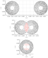 |
Fig. 1. Geometry and kinematics of the SMBBH for each model. From top to bottom panels: distant, contact, and mixed. Black arrows show the non-perturbed velocity field, while red ones are for clumps with an additional random component of the velocity. |
Additionally, we simulated two models with mass ratio q = 0.5 and q = 0.1 for this case. Assuming that photoionization and recombination following radiative de-excitation is the main mechanism for the emission of broad Balmer lines, the BLR size scales with luminosity in the form of RBLR ∝ L0.5 (Kaspi et al. 2005). We used the mass luminosity relation MBH ∝ L0.7 (Woo & Urry 2002) in order to obtain the BLR size depending solely on mass of each component. An illustration for these two cases is shown in Fig. 2.
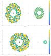 |
Fig. 2. Distant model with mass ratio q = 0.5 (upper panel) and with q = 0.1 (lower panel). The black cross shows the center of mass, while the blue asterisk marks the L1 Lagrangian point. The color bar denotes the vertical offset from the xy plane. |
Contact. Black holes are separated by a = 16.7 light days with orbital period of 15.5 years, which allows for certain parts of the BLRs to overlap (Fig. 1, middle panel). In this regime, the BLR kinematics is similar to the previous model, except for the overlapping part where we assigned a chaotic component to the velocity for each clump due to chocks, stirring, and inelastic collisions.
Mixed. For this model, the black holes are much closer to each other, at an orbital separation of three light days and with an orbital period of 1.2 years. In Fig. 1, third panel, clumps in red are the ones with an additional chaotic component, while for the rest we calculated velocity as if in the center was a single SMBH with mass equal to the sum of the binary components.
Spiral. Hydrodynamic simulations involving subparsec SMBBHs have shown that black holes are surrounded by a common circumbinary (CB) disk. Accreting gas around the binaries forms a low density cavity inside the CB disk (MacFadyen & Milosavljević 2008; Cuadra et al. 2009). We found that the accretion streams are in the form of spiral arms with higher density, which connects the mini accretion disk of each black hole with the surrounding CB disk (Noble et al. 2012; Shi & Krolik 2015). In this scenario, the cavity is of the order of a, and the CB disk extends from 1.5a to 3a. Following a similar setup to Smailagić & Bon (2015), we built a SMBBH model with spiral arms and the surrounding CB disk in order to investigate the polarization signatures coming from the SMBBH. We keep the same mass of each component as 5 × 10⁷ M⊙ with the orbital separation the same as in the case for contact model, a = 16.7 light days. We approximated spiral arms with logarithmic spirals with boundaries in polar coordinates given as
where b and B are parameters that describe the wrapping of the spirals. We chose wrapping parameters of B = 0.55 and b = 0.45. This set of parameters for b and B was chosen in order to have two distinct spirals with single winding and to avoid the mixture or interaction of the spirals. We chose the half-opening angle for the spirals and the CB disk to be 20°. An illustration of the model is shown in Fig. 3. For the kinematics of the spirals, we used the rotation of an absolutely rigid body, that is, the spirals are stationary in the rotating reference frame of the SMBBH. The CB is under the Keplerian motion around the common center of mass. The system is again surrounded by the same scattering region as in previous models, with the same radial optical depth in the equatorial plane.
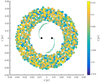 |
Fig. 3. SMBBHs (black circles) with spiral arms surrounded by a CB disk. Each spiral is modeled with 500 clumps. The CB is modeled with 1000 clumps. The color bar denotes the vertical offset from the xy plane. |
The BLR is represented by thousands of clumps. The volume filling factor of the BLR is 0.25, as constrained from simulations and observations (Marin et al. 2015). The total number of clumps per model, as well as the other parameters used in the model, are listed in Table 1.
Description of the three SMBBH models.
2.1. Scattering region
Optical continuum and line polarization properties typically found in Type-1 objects can be produced by electron scattering of a flattened distribution that is surrounding the accretion disk and the BLR (Antonucci 1984; Smith et al. 2005). The scattering region is modeled with flared-disk geometry with an inner and outer radius of 0.1 and 0.5 parsec. The half-opening angle is 30° with respect to the equatorial plane. Electron concentration is chosen in such a way that the total radial optical depth in the equatorial plane for Thomson scattering is three, which is enough to produce a typical degree of polarization that is found in Type-1 objects (Marin et al. 2012). An illustration of the scattering region surrounding the central engine is illustrated on Fig. 4.
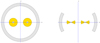 |
Fig. 4. Cartoon illustrating equatorial scattering region. The left figure shows the face-on view, while on the right the same geometry is shown when viewed edge-on. An example is shown for the case in which the two BLRs are separated. The BLRs are shown in yellow. The scattering region is shown in gray. |
2.2. Numerical simulations
Assuming that AGN polarization arises predominantly from scattering in non-jetted systems, we apply full 3D radiative transfer with polarization using the publicly available code, STOKES (Goosmann & Gaskell 2007; Marin et al. 2012, 2015; Marin 2018; Rojas Lobos et al. 2018). It is based on a Monte Carlo algorithm, for which a vast literature already exist, and with 3D kinematics fully implemented in spherical coordinates. The code follows the trajectory of each photon through the model space, from their creation until they are registered by the web of virtual detectors positioned all over the sky. The net Stokes parameters I, Q, U, and V are thus determined and other physical quantities may be inferred, namely degree of linear polarization (PO), polarized flux (PF), and polarization position angle (φ). Originally, the code was developed for studying optical and UV scattering-induced continuum polarization in the radio-quiet AGN, but nowadays it is widely used for studying the polarization of many astrophysical phenomena (Marin & Goosmann 2014). We used the intermediate 2.04 version of STOKES, which is not yet publicly available2. We adopt the same convention as Goosmann & Gaskell (2007): we defined φ to be 0° when the polarization angle is perpendicular to the projected symmetry axis of the model. When φ is 90°, the polarization angle is parallel to the symmetry axis of the model.
3. Results
We simulated the different SMBBH scenarios presented in the previous section with different kinematics of the BLR depending on the model. In the following, we thoroughly investigate the results for each case. For clarity and easy comparison, we present the results of a model with a single SMBH in the center with mass Mbh = 108 M⊙, so the reader could have a clearer picture when comparing the results for a single SMBH scenario with a SMBBH. The result of the single SMBH model is given in Fig. 5, the results for a SMBBH with the same center of mass in Fig. 6, and the numerous results for all the SMBBH scenarios are shown in Appendix A.
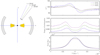 |
Fig. 5. Left panel: illustration of the model with a single SMBH in the center surrounded by a BLR (yellow) and the scattering region (gray) is shown. Right panel: profiles of polarization angle (top panel), the degree polarization (middle panel), and the total flux (bottom panel) when viewed from two intermediate inclinations. The polarization angle is given in degrees (°). We point out that the degree of polarization is given as fraction units and is lower than the ones we obtain in the following section due to the different size and optical depth of the scattering region. The total flux is given in arbitrary units. Model parameters are the same as the ones given by Savić et al. (2018). |
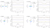 |
Fig. 6. Left panels: illustration of each model with SMBBH in the center: Distant (panel a), contact (panel b), mixed (panel c), and spiral (panel d). Right panels, from top to bottom: φ, PO, and TF for two viewing inclinations and for azimuthal viewing angle ϕ = 18°. |
For Type-1 objects, for a single case scenario – a single black hole and a single BLR surrounded by a dusty torus – in the case for equatorial scattering, the φ shows symmetric swing around the line center (Smith et al. 2005; Afanasiev et al. 2014; Afanasiev & Popović 2015; Savić et al. 2018). This feature was very well observed in few objects (e.g., Mrk 6, NGC 4051, NGC 4151) and can be used for measuring masses of SMBHs using the polarization of broad-line profiles (Afanasiev et al. 2014; Afanasiev & Popović 2015; Savić et al. 2018).
3.1. Distant
In Figs. 6 (panel a) and A.1 we show the simulated φ-profiles for two viewing inclinations i and for different azimuthal viewing angles ϕ. We can see that profiles of φ are complex and differ much from the profiles for the single black hole scenario. For a fixed viewing ϕ, the φ-profiles show similar profiles with the peaks most prominent when viewed towards face-on inclinations. For different azimuthal viewing angles, φ-profiles are quite diverse. This diversity is the result of different velocity projections toward the observer since the model is not azimuthally symmetric. The φ-profiles are symmetric with respect to the line center, which is not the case for a single case scenario where the swing occurs.
The typical degree of polarization (PO) found for Type-1 objects is around 1% or less. Our simulations show that PO is in the range between 1% and 4% (Fig. A.2). This unusually high PO is due to the high radial optical depth of the scattering region. It is inclination dependent and it is increasing when observing from face-on toward edge-on viewing inclinations, as expected from Thomson’s law. For some ϕ (Fig. A.2, top left and bottom right panels), the PO profile peaks in the line wings and has a minimum value in the line core. This is the same as in the case for a single black hole scenario and has been confirmed observationally (e.g., Mrk 6, Smith et al. 2002; Afanasiev et al. 2014). However, this is not the case for all ϕ and we can see the opposite situation in which PO peaks in the line core and is minimum in the line wings.
The total flux (TF) shows variability in the line profiles (Fig. A.3). Line profiles are sensitive both to viewing inclinations and viewing azimuthal angles. In general, double-peaked profiles are observed, with line width being broader when observing from face-on towards edge-on inclinations. Line widths are different with respect to ϕ with the broadest lines observed for ϕ = 90° or ϕ = 270° (Fig. A.3, middle upper and bottom panels). Some viewing angles show single-peak lines (Fig. A.3, top left and bottom right panels) and the corresponding PO profiles are as in the case for a single black hole scenario. This means that in the certain orbital phase, we would not be able to observationally distinguish between the SMBBHs and SMBHs from the unpolarized optical spectra. However, for this case, φ shows a different profile than expected, which could provide more insight if the SMBBHs are situated in the center.
For the distant model, with mass ratio q = 0.5, we can expect asymmetric profiles for φ, PO, and TF (Figs. A.4–A.6). The φ has similar profiles as for the case with mass ratio q = 1, except that peaks are not symmetric and they have different intensities. When compared with the previous case, the φ-profile is similar except for azimuthal viewing angles ϕ = 224° where the profile is flat in the core (Fig. A.4, lower left panel), or an additional swing can be noticed in the core for ϕ = 342° (Fig. A.4, upper right panel).
The degree of polarization has profiles with the same shape as for the previous case except that they are asymmetric and it is the case for all viewing angles. We obtained the same order of polarization with the same inclination dependency (Fig. A.5).
The unpolarized line shows a displaced single peak profile when viewed almost face-on for most of the azimuthal viewing angles, except when ϕ = 224° and 270° where a clear double-peaked profile can be observed (Fig. A.6, bottom left and middle panels). For intermediate inclinations, line profiles are asymmetric with double peaks and with different line shifts depending on the azimuthal viewing angles (Fig. A.6).
For the same model with q = 0.1, we obtained similar profiles as before for φ, PO, and TF (Figs. A.7–A.9), however, they are more asymmetric than for the case with q = 0.5. The φ has similar profiles as for the cases with q = 1 and q = 0.5 with asymmetry highlighted (Fig. A.7).
The degree of polarization shows profiles with the same shape in the same way as before for all viewing angles. Polarization is of the same order with the same inclination dependency (Fig. A.8).
The unpolarized flux shows complex asymmetric profiles with line peaks having different positions as the system is viewed in different orbital phases (Fig. A.9). When q = 0.1, the more massive component has a smaller orbital velocity and it is much smaller compared to the Keplerian velocity of the BLR clouds surrounding it. For the less massive component, orbital velocity is of the same order in comparison to the Keplerian velocity of the BLR clouds surrounding it, which contributes to higher line shift. With these two effects combined, we observe highly asymmetric line profiles that significantly vary with the orbital phase.
3.2. Contact
This scenario is geometrically similar to the previous one, with the SMBBHs being closer and allowing an additional chaotic velocity component that will affect the line profile mostly around its core. The simulated φ is shown on Figs. 6 (panel b) and A.10. The φ profiles are also similar to the case of separated BLRs. Figure A.10 (left panels; upper and middle right) clearly show two minima in the wings and a maximum in the line core; or a minimum in the line core and maximum in the line wings. The observed φ profile is the most sensitive to random velocity when the system is viewed from ϕ = 90° and ϕ = 270° (Fig. A.10, middle up and bottom panels), for which we observe two minima and an almost flat profile in the core. For ϕ = 342° (Fig. A.10, bottom right panel), we see one peak in the red wing for the near face-on viewing i, while the profile is almost constant for the intermediate inclination. We expect that an additional chaotic velocity component will affect the profile, mostly at the core, which is exactly what we get from the models.
In Fig. A.11 the resulting PO is shown. The degree of polarization is in the same range as it was for the previous case. Again, PO increases when viewing from face-on toward edge-on inclinations.
The total flux is largely affected by the additional random motion of the BLR clouds in the line core (Fig. A.12). We can clearly observe double-peaked lines for intermediate inclinations (i = 38° and i = 41°, Fig. A.12, upper panels and bottom left and middle panels). For ϕ = 18 ° ,198°, and 342° (Fig. A.12), we observe single-peak profiles, and for intermediate inclinations, line cores are flattened. The highest line widths are for ϕ = 90° and ϕ = 270°.
3.3. Mixed
When the two BLRs are mixed and surround both black holes, we can observe that the change of φ is small with the respect to the continuum level (Figs. 6 (panel c) and A.13) and it is the highest for nearly face-on inclinations. For intermediate inclinations, the φ profiles could be considered as constant with additional noise. This is expected since the largest fraction of flux is coming from the clouds, with additional random velocity components that are close to the black holes.
Figure A.14 shows the resulting PO for a set of viewing inclinations and azimuthal angles. We can see that the broad-line profiles are almost flat with very low characteristic features. We obtain the same range for PO as in the previous models.
The total flux shows seemingly complex profiles (Fig. A.15) with multiple spikes. However, this is due to the fact that we are very much limited to the number of BLR clouds when running the simulations. Running the STOKES code with more than 5000 individual clouds would be impractical and extremely time consuming. These results are in agreement with the ones obtained by Smith et al. (2005); we can see that, when applied to a large number of BLR clouds, an additional random velocity component plus the Keplerian component tend to smooth and flatten the resulting spectra. We obtain flat profiles for φ and PO, and we can expect a single-peaked line.
3.4. Spiral
In Figs. 6 (panel d) and A.16, the results for φ for the spiral model are shown. The simulated φ shows double-peak profiles, with minima or maxima occurring around V ≈ 3000 km s−1 for all i and ϕ. This velocity is close to the orbital velocity of each binary component for which V ≈ 2800 km s−1. This result is due to the majority of the emitted flux that originates from the inner parts of the spiral arms closer to the black holes, and due to the velocity of the rigid body scaling with the distance. The intensity of the peaks is inclination dependent and decreases when the system is viewed from face-on toward edge-on inclinations.
In Fig. A.17 the results for the simulated PO are shown. We can see that PO has similar profiles to φ – visible peaks in the line wings and minimum in the line core (Fig. A.17, left upper and middle panels; right bottom and middle panels), which is characteristic for a single black hole scenario, or the opposite profiles, with maximum PO in the line core and minimum in the wings.
The results for TF are shown in Fig. A.18. We can see various line profiles for different ϕ. For intermediate inclinations, we observe double-peaked line profiles. For near face-on viewing angles and some ϕ, profiles with a strong single peak (Fig. A.18, bottom right panel), or two peaks very close to each other (Fig. A.18, middle left and right panels) are observed.
4. Discussion
4.1. Overview of our results
The presence of another BLR (as in the case of our model) has a unique signature on the simulated φ-profiles for all the models we tested. A double-peaked feature can be observed, and the φ-profile varies drastically depending on the observed orbital phase of the system and it is different from the case of a single SMBH. This is always the case for PO and TF, which often show complex profiles. However, in some cases, when viewed from certain azimuthal viewing angles, the simulated PO and TF profiles are very similar for the case with a single SMBH in the center. AGN monitoring is therefore required to distinguish between these two cases. We have seen that additional random motion tends to smooth the profiles of TF in the line core, while diluting φ-profiles. The total flux is also largely dependent on the observed phase of the binary system. Lines show complex varying profiles, and long-term monitoring spectroscopy combined with spectropolarimetry could prove very useful in the search for SMBBH candidates. In order to see the variability in the line, we are limited only to close subparsec SMBBHs for which the half-period of revolution is of the order of up to a few tens of years. Less massive SMBBHs or the ones with greater orbital distance would yield orbital periods of the order of a few centuries, the line profile change of which would be impractical to observe.
In Savić et al. (2018), we simulated equatorial scattering with additional complex (inflows/outflows) motion in the BLR for a single SMBH in the center. The φ-profiles show point (central) symmetry for all treated cases (e.g., a prominent minimum followed by a maximum of the same amplitude), while the TF remains axisymmetric with the respect to the line center. Smith et al. (2005) have included inflows and high-velocity rotation in the scattering region and this yielded complex but again point-symmetric φ-profiles. Depending on the model, our simulations involving SMBBHs as a result have axisymmetric φ-profiles. This behavior of the polarization angle may prove crucial as a distinct feature in the search for SMBBHs.
4.2. AGN with double-peaked emission line profiles
Broad emission line profiles and line variability can be explained by a wide variety of different kinematic models that would yield similar results. Naturally, AGN with variable double-peaked lines make good targets for spectropolarimetric observations and long-term monitoring campaigns. We discuss our results with observations of three well-known double-peaked AGN: NGC 1097, 3C 390.3, and Arp 102B.
Spectral optical monitoring of Arp 102B over the period from 1987 to 2010 shows no significant change in the broad double-peaked Hα and Hβ profiles (Shapovalova et al. 2013; Popović et al. 2014). The Hβ line is broader than Hα during the monitored period and both can be well reproduced by a disk model. However, spectropolarimetric observations are partially inconsistent with the disk model (Corbett et al. 1998, 2000). The Hα polarization angle has almost the same value as the angle of the jet direction, which is in good agreement with equatorial scattering. The observed single-peak profile of the polarized line with respect to the unpolarized line suggests that the BLR clouds might be undergoing biconical outflows (Antonucci et al. 1996; Corbett et al. 1998, 2000). The φ-profile is flat without any distinctive features.
The active galaxy 3C 390.3 is a well-known source with remarkably strong variability in the X-ray, UV, and optical regime (see Afanasiev et al. 2015, and the references therein). The unpolarized and polarized flux are quite different. The unpolarized Hα has a double-peaked profile with the blue peak being more prominent. The polarized Hα is single-peaked and shifted to blue for 1200 km s−1 with the respect to the narrow component, and is strongly depolarized in the center (Afanasiev et al. 2015). A model with biconical outflows (Corbett et al. 2000) for this object is not in agreement with the optical monitoring of the BLR. The cross-correlation (CCF) analysis by Afanasiev et al. (2015) for Hα and Hβ shows no significant delay in the variation between the blue and the red line wings relative to each other or with the respect to the line core. This is in favor of a model in which the BLR originates from an accretion disk with dominant Keplerian motion. A two-component BLR model with a disk and an outflowing region can explain well spectropolarimetric observations. In this model, an outflowing region is located above the disk and it can depolarize the radiation emitted from the disk.
Optical monitoring of NGC 1097 between 1991 and 1996 has shown a peculiar evolution of the Hα line profile. The broad Hα double peak showed a red-peak dominance (Storchi-Bergmann et al. 1993), followed by a nearly symmetrical profile (Storchi-Bergmann et al. 1995) and up to a blue-peak dominant profile (Storchi-Bergmann et al. 1997). A model of a precessing elliptical ring around the SMBH (Eracleous et al. 1995) was used to explain the observed line profiles and to fit the data. In this model it was proposed that the origin of the elliptical disk is due to the tidal disruption of a star by a SMBH or it could be due to the existence of a SMBBH. In both cases, the broad line variability that could be observed is of the order of a few years when the total mass is smaller than 106 M⊙. For SMBH with mass of the order of 108 M⊙, which is the case for NGC 10973, the precession period is of the order of a few centuries and could not be observed. However, in the scenario we studied, where each component has a separate accretion disk surrounded by the BLR, the variability of the order of a few years could be observed if the binary system is close enough. Line variability would show systematic periodicity and it is attributed only to the viewed orbital phase of the system. In order to fit the observational data with our model, a large grid of models needs to be constructed. Besides the main parameters of the model such as total mass, orbital distance, mass ratio, the parameter space would also include luminosities and BLR sizes of each component along with the parameters describing the scattering region as well as the optical depth. This is well beyond the scope of the present work and limits our investigation, which is based on a simple model.
When viewed in polarized light, NGC 1097 shows a weak continuum polarization (p = 0.26 ± 0.02%) in the optical domain over 5100–6100 Å (Barth et al. 1999). The Hα line also shows weak polarization and no characteristic feature for a single or binary BH could be detected in the PO and PF profiles. New high-quality spectropolarimetric observations are thus required in order to confirm our results.
AGN with unpolarized double-peaked profiles with varying red and blue peaks with respect to each other are probably the best candidates in the search for SMBBHs. Although a single SMBH in the center of AGN is the most probable case, SMBBH in the central engine should have their distinctive signature in the polarized spectra due to the polarization sensitivity to the geometry and kinematics.
5. Conclusions
We investigated the polarization signatures of SMBBHs in AGN using a set of simple yet representative models. We assumed equatorial scattering as a main mechanism for optical polarization and we used the Monte Carlo code STOKES to solve 3D polarized radiative transfer with kinematics. We used simple geometry for polarization modeling of SMBBHs in AGN and we treated four different cases in which the BLRs have different geometry: distant, contact, mixed, and spiral. We outline the characteristic features of φ, PO and TF that are in common for all the models we studied. The polarization position angle φ shows double-peaked or even more complex profiles most of the time. The PO shows double-peaked profiles with minimum in the line core, which is common for the single SMBH scenario, but there are opposite profiles with minima in the line wings and maximal PO in the line core, which may be an indicator of a SMBBHs. Most of the time, the TF shows double- or multi-peaked profiles, which are often associated with the disk profiles. The combined results of all of our simulations involving SMBBHs lead to the following two conclusions:
-
The degree of polarization and total flux, along with the unique profiles characteristic of SMBBHs also show profiles that are common for single SMBHs and alone may prove inconclusive for disentangling the central engine of AGN.
-
On the other hand, the polarization position angle φ shows quite different and unique profiles from the ones observed for the single SMBH scenario, and the inspection of these could be used as a first step for finding SMBBH candidates.
We demonstrated that when a SMBBH is situated in the center of Type-1 AGN, spectropolarimetry could be a powerful tool for searching for the SMBBH candidates amongst them. In this paper we assumed that the accretion disks of the two black holes are coplanar and that they are coplanar with the torus, that is, the scattering region. Our assumption of coplanarity is very well supported by previous results from high-resolution hydrodynamical simulations. However, for a general picture of how significant the orientation between the disks in the short-lived phase and misaligned disks is, a more detailed analysis with the expanded model space grid is required. With the results obtained so far, in this case, we expect to have highly asymmetric profiles of the total flux and the degree of polarization, while for the polarization position angle, we expect to have lower amplitude and flatter profiles. We intend to explore the cases of non-coplanarity in a follow-up paper that will investigate the whole (and large) phase space of free parameters.
The quasar has highly shifted Balmer lines around 1000 km s−1 and a red asymmetry (see Shapovalova et al. 2016).
Mbh = (1.2 ± 0.2)×108 M⊙ (Lewis & Eracleous 2006); Mbh = (1.40 ± 0.32)×108 M⊙ (Onishi et al. 2015).
Acknowledgments
This work was supported by the Ministry of Education and Science (Republic of Serbia) through the project Astrophysical Spectroscopy of Extragalactic Objects (176001), the French PNHE, and the grant ANR-11-JS56-013-01 “POLIOPTIX”. F. M. is grateful to the Centre national d’études spatiales (CNES) and its post-doctoral grant “Probing the geometry and physics of active galactic nuclei with ultraviolet and X-ray polarized radiative transfer”. D. Savić thanks the French Government and the French Embassy in Serbia for supporting his research without which this work would not be possible.
References
- Abbott, B. P., Abbott, R., Abbott, T. D., et al. 2016, Phys. Rev. Lett., 116, 061102 [Google Scholar]
- Afanasiev, V. L., & Popović, L. Č. 2015, ApJ, 800, L35 [Google Scholar]
- Afanasiev, V. L., Popović, L. Č., Shapovalova, A. I., Borisov, N. V., & Ilić, D. 2014, MNRAS, 440, 519 [Google Scholar]
- Afanasiev, V. L., Shapovalova, A. I., Popović, L. Č., & Borisov, N. V. 2015, MNRAS, 448, 2879 [NASA ADS] [CrossRef] [Google Scholar]
- Antonucci, R. R. J. 1984, ApJ, 278, 499 [NASA ADS] [CrossRef] [Google Scholar]
- Antonucci, R., Hurt, T., & Agol, E. 1996, ApJ, 456, L25 [NASA ADS] [Google Scholar]
- Barth, A. J., Filippenko, A. V., & Moran, E. C. 1999, ApJ, 525, 673 [NASA ADS] [CrossRef] [Google Scholar]
- Begelman, M. C., Blandford, R. D., & Rees, M. J. 1980, Nature, 287, 307 [NASA ADS] [CrossRef] [Google Scholar]
- Bogdanović, T., Reynolds, C. S., & Miller, M. C. 2007, ApJ, 661, L147 [NASA ADS] [CrossRef] [Google Scholar]
- Bon, E., Jovanović, P., Marziani, P., et al. 2012, ApJ, 759, 118 [NASA ADS] [CrossRef] [Google Scholar]
- Boroson, T. A., & Lauer, T. R. 2009, Nature, 458, 53 [NASA ADS] [CrossRef] [PubMed] [Google Scholar]
- Capriotti, E., Foltz, C., & Byard, P. 1979, ApJ, 230, 681 [NASA ADS] [CrossRef] [Google Scholar]
- Corbett, E. A., Robinson, A., Axon, D. J., Young, S., & Hough, J. H. 1998, MNRAS, 296, 721 [NASA ADS] [CrossRef] [Google Scholar]
- Corbett, E. A., Robinson, A., Axon, D. J., & Young, S. 2000, MNRAS, 319, 685 [NASA ADS] [CrossRef] [Google Scholar]
- Cuadra, J., Armitage, P. J., Alexander, R. D., & Begelman, M. C. 2009, MNRAS, 393, 1423 [NASA ADS] [CrossRef] [Google Scholar]
- Dobbie, P. B., Kuncic, Z., Bicknell, G. V., & Salmeron, R. 2009, Plasma Fusion Res., 4, 017 [NASA ADS] [CrossRef] [Google Scholar]
- Dotti, M., Volonteri, M., Perego, A., et al. 2010, MNRAS, 402, 682 [NASA ADS] [CrossRef] [Google Scholar]
- Eracleous, M., & Halpern, J. P. 2003, ApJ, 599, 886 [NASA ADS] [CrossRef] [Google Scholar]
- Eracleous, M., Livio, M., Halpern, J. P., & Storchi-Bergmann, T. 1995, ApJ, 438, 610 [NASA ADS] [CrossRef] [Google Scholar]
- Eracleous, M., Lewis, K. T., & Flohic, H. M. L. G. 2009, New Astron. Rev., 53, 133 [NASA ADS] [CrossRef] [Google Scholar]
- Eracleous, M., Boroson, T. A., Halpern, J. P., & Liu, J. 2012, ApJS, 201, 23 [NASA ADS] [CrossRef] [Google Scholar]
- Gaskell, C. M. 1983, in Liege International Astrophysical Colloquia, ed. J. P. Swings, 24, 473 [NASA ADS] [Google Scholar]
- Gaskell, C. M. 2008, Rev. Mex. Astron. Astrofis. Conf. Ser., 32, 1 [NASA ADS] [Google Scholar]
- Gaskell, C. M. 2009, New Astron. Rev., 53, 140 [NASA ADS] [CrossRef] [Google Scholar]
- Gaskell, C. M., & Klimek, E. S. 2003, Astron. Astrophys. Trans., 22, 661 [NASA ADS] [CrossRef] [Google Scholar]
- Goosmann, R. W., & Gaskell, C. M. 2007, A&A, 465, 129 [NASA ADS] [CrossRef] [EDP Sciences] [Google Scholar]
- Goosmann, R. W., Gaskell, C. M., & Marin, F. 2014, Adv. Space Res., 54, 1341 [NASA ADS] [CrossRef] [Google Scholar]
- Graham, M. J., Djorgovski, S. G., Stern, D., et al. 2015, MNRAS, 453, 1562 [NASA ADS] [CrossRef] [Google Scholar]
- Kaspi, S., Maoz, D., Netzer, H., et al. 2005, ApJ, 629, 61 [NASA ADS] [CrossRef] [Google Scholar]
- Kormendy, J., & Ho, L. C. 2013, ARA&A, 51, 511 [Google Scholar]
- Kormendy, J., & Richstone, D. 1995, ARA&A, 33, 581 [NASA ADS] [CrossRef] [Google Scholar]
- Landau, L., & Lifshitz, E. 1969, Mechanics, Ch. VII (Oxford: Pergamon Press) [Google Scholar]
- Lewis, K. T., & Eracleous, M. 2006, ApJ, 642, 711 [NASA ADS] [CrossRef] [Google Scholar]
- Li, Y.-R., Wang, J.-M., Ho, L. C., et al. 2016, ApJ, 822, 4 [Google Scholar]
- MacFadyen, A. I., & Milosavljević, M. 2008, ApJ, 672, 83 [Google Scholar]
- Marin, F. 2018, A&A, 615, A171 [NASA ADS] [CrossRef] [EDP Sciences] [Google Scholar]
- Marin, F., & Goosmann, R. W. 2014, in SF2A-2014: Proceedings of the Annual meeting of the French Society of Astronomy and Astrophysics, eds. J. Ballet, F. Martins, F. Bournaud, R. Monier, & C. Reylé, 103 [Google Scholar]
- Marin, F., Goosmann, R. W., Gaskell, C. M., Porquet, D., & Dovčiak, M. 2012, A&A, 548, A121 [NASA ADS] [CrossRef] [EDP Sciences] [Google Scholar]
- Marin, F., Goosmann, R. W., & Gaskell, C. M. 2015, A&A, 577, A66 [Google Scholar]
- Mayer, L., Kazantzidis, S., Escala, A., & Callegari, S. 2010, Nature, 466, 1082 [NASA ADS] [CrossRef] [Google Scholar]
- Meyers, K. A., & Peterson, B. M. 1985, PASP, 97, 734 [NASA ADS] [CrossRef] [Google Scholar]
- Miller, M. C., & Krolik, J. H. 2013, ApJ, 774, 43 [NASA ADS] [CrossRef] [Google Scholar]
- Milosavljević, M., & Merritt, D. 2003, in The Astrophysics of Gravitational Wave Sources, ed. J. M. Centrella, Am. Inst. Phys. Conf. Ser., 686, 201 [NASA ADS] [CrossRef] [Google Scholar]
- Netzer, H. 1990, in Active Galactic Nuclei, eds. R. D. Blandford, H. Netzer, L. Woltjer, T. J. L. Courvoisier, & M. Mayor, 57 [Google Scholar]
- Netzer, H. 2013, The Physics and Evolution of Active Galactic Nuclei (Cambridge University Press) [CrossRef] [Google Scholar]
- Nguyen, K., & Bogdanović, T. 2016, ApJ, 828, 68 [NASA ADS] [CrossRef] [Google Scholar]
- Noble, S. C., Mundim, B. C., Nakano, H., et al. 2012, ApJ, 755, 51 [NASA ADS] [CrossRef] [Google Scholar]
- Onishi, K., Iguchi, S., Sheth, K., & Kohno, K. 2015, ApJ, 806, 39 [NASA ADS] [CrossRef] [Google Scholar]
- Peterson, B. M., Ferrarese, L., Gilbert, K. M., et al. 2004, ApJ, 613, 682 [NASA ADS] [CrossRef] [Google Scholar]
- Piotrovich, M. Y., Gnedin, Y. N., Natsvlishvili, T. M., & Buliga, S. D. 2017, Ap&SS, 362, 110 [NASA ADS] [CrossRef] [Google Scholar]
- Popović, L. Č. 2012, New Astron. Rev., 56, 74 [Google Scholar]
- Popovic, L. C., Mediavilla, E. G., & Pavlovic, R. 2000, Serb. Astron., J, 162 [Google Scholar]
- Popović, L. Č., Shapovalova, A. I., Ilić, D., et al. 2014, A&A, 572, A66 [NASA ADS] [CrossRef] [EDP Sciences] [Google Scholar]
- Robinson, A., Young, S., Axon, D. J., Kharb, P., & Smith, J. E. 2010, ApJ, 717, L122 [NASA ADS] [CrossRef] [Google Scholar]
- Rojas Lobos, P. A., Goosmann, R. W., Marin, F., & Savić, D. 2018, A&A, 611, A39 [NASA ADS] [CrossRef] [EDP Sciences] [Google Scholar]
- Savić, D., Goosmann, R., Popović, L. Č., Marin, F., & Afanasiev, V. L. 2018, A&A, 614, A120 [NASA ADS] [CrossRef] [EDP Sciences] [Google Scholar]
- Shannon, R. M., Ravi, V., Lentati, L. T., et al. 2015, Science, 349, 1522 [NASA ADS] [CrossRef] [Google Scholar]
- Shapovalova, A. I., Popović, L. Č., Burenkov, A. N., et al. 2013, A&A, 559, A10 [NASA ADS] [CrossRef] [EDP Sciences] [Google Scholar]
- Shapovalova, A. I., Popović, L. Č., Chavushyan, V. H., et al. 2016, ApJS, 222, 25 [NASA ADS] [CrossRef] [Google Scholar]
- Shemmer, O., Netzer, H., Maiolino, R., et al. 2004, ApJ, 614, 547 [NASA ADS] [CrossRef] [Google Scholar]
- Shen, Y., & Loeb, A. 2010, ApJ, 725, 249 [NASA ADS] [CrossRef] [Google Scholar]
- Shi, J.-M., & Krolik, J. H. 2015, ApJ, 807, 131 [NASA ADS] [CrossRef] [Google Scholar]
- Simić, S., & Popović, L. Č. 2016, Ap&SS, 361, 59 [NASA ADS] [CrossRef] [Google Scholar]
- Smailagić, M., & Bon, E. 2015, JApA, 36, 513 [NASA ADS] [Google Scholar]
- Smith, J. E., Young, S., Robinson, A., et al. 2002, MNRAS, 335, 773 [NASA ADS] [CrossRef] [Google Scholar]
- Smith, J. E., Robinson, A., Young, S., Axon, D. J., & Corbett, E. A. 2005, MNRAS, 359, 846 [NASA ADS] [CrossRef] [Google Scholar]
- Storchi-Bergmann, T., Baldwin, J. A., & Wilson, A. S. 1993, ApJ, 410, L11 [NASA ADS] [CrossRef] [Google Scholar]
- Storchi-Bergmann, T., Eracleous, M., Livio, M., et al. 1995, ApJ, 443, 617 [NASA ADS] [CrossRef] [Google Scholar]
- Storchi-Bergmann, T., Eracleous, M., Teresa Ruiz, M., et al. 1997, ApJ, 489, 87 [NASA ADS] [CrossRef] [Google Scholar]
- Vika, M., Driver, S. P., Graham, A. W., & Liske, J. 2009, MNRAS, 400, 1451 [NASA ADS] [CrossRef] [Google Scholar]
- Volonteri, M., Haardt, F., & Madau, P. 2003a, ApJ, 582, 559 [NASA ADS] [CrossRef] [Google Scholar]
- Volonteri, M., Madau, P., & Haardt, F. 2003b, ApJ, 593, 661 [NASA ADS] [CrossRef] [Google Scholar]
- Walker, S. A., Fabian, A. C., Russell, H. R., & Sanders, J. S. 2014, MNRAS, 442, 2809 [NASA ADS] [CrossRef] [Google Scholar]
- Woo, J.-H., & Urry, C. M. 2002, ApJ, 579, 530 [NASA ADS] [CrossRef] [Google Scholar]
- Zuo, W., Wu, X.-B., Fan, X., et al. 2015, ApJ, 799, 189 [NASA ADS] [CrossRef] [Google Scholar]
Appendix A: Detailed results of modeling
Simulations for all models are presented in Figs. A.1–A.18. The simulated profiles for φ, PO, and TF are given for two viewing inclinations: i ≈ 18° and 32°. Azimuthal viewing angles take eight values: ϕ = 18°, 54°, 90°, 126°, 198°, 224°, 270°, and 342°. The results are given as a function of velocity defined as V = c(λ − λ0)/λ0, where λ is wavelength and λ0 is the central wavelength of a given spectral line. The broad-line region for each model is shown in the center of every image. Arrows represent the velocity field of the BLR. For each model, we outline the main features for completeness.
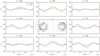 |
Fig. A.1. Simulated profiles of φ across the line profile for two viewing inclinations i when observed from different azimuthal angles ϕ. Geometry and kinematics of the model are in the center for clarity. |
Distant. This case is shown in Figs. A.1–A.3 for mass ratio q = 1. In Fig. A.1 the polarization angle φ is shown. We can observe double-peaked profiles of φ that drastically vary depending on the orbital phase of the system. For ϕ = 18° and 198°, φ reaches maximum values in the line wings and minimum in the core, while for ϕ = 90° and ϕ = 270°, it is the opposite way around. The PO is shown in Fig. A.2 and shows similar profiles to φ, but they are not correlated. Profiles with minimum in the core and maxima in the wings, which is common for the single SMBH scenario, can be seen for ϕ = 126° and 342°. The opposite profiles are for ϕ = 18°, 54°, 198°, and 234°. The TF is shown in Fig. A.3. Double-peaked profiles can be seen for ϕ = 18°, 54°, 198°, and 234° and for all viewing inclinations. Single-peaked profiles are for ϕ = 342° and ϕ = 126°.
The results of the same model for mass ratio q = 0.5 are shown in Figs. A.4–A.6. The φ and PO are shown in Figs. A.4–A.5 respectively; both follow the same trend as for the case with mass ratio q = 1 and both show mild asymmetry in the profiles. The TF (Fig. A.6) shows asymmetric double-peak or single-peak profiles with the positions of the peaks varying depending on the observed orbital phase of the system. For q = 0.1, simulated profiles for φ, PO, and TF are shown in Figs. A.7–A.9. The results are very similar to the previous case with remarkable asymmetry in the profiles.
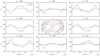 |
Fig. A.10. Same as Fig. A.1, but for contact model. |
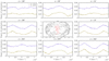 |
Fig. A.11. Same as Fig. A.10, but for PO. |
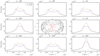 |
Fig. A.12. Same as Fig. A.10, but for TF. |
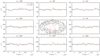 |
Fig. A.13. Same as Fig. A.1, but for mixed model. |
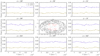 |
Fig. A.14. Same as Fig. A.13, but for PO. |
Contact. The results for this model are shown in Figs. A.10–A.12. The φ-profiles are shown in Fig. A.10 for different orbital phases of the system. Profiles are very similar to the ones obtained for the distant model, but with greater amplitude of maxima and minima. The PO profiles are shown in Fig. A.11. For ϕ = 18°, 198°, and 342°, the profiles are the same as for the single SMBH scenario, while for all the other azimuthal viewing angles, the maximum PO is in the line core. The TF is shown in Fig. A.12. Lines are broadest when viewed for ϕ = 90° and 270°. The random velocity component in this model, which is present in the BLR, flattens the line profiles, making it difficult to distinguish between single-peaked and double-peaked profiles.
Mixed. Simulations for this model are shown in Figs. A.13–A.15. The polarization angle is shown in Fig. A.13. The φ-profiles are double-peaked for ϕ = 18°, 126°, and 198°. A swing in the φ-profile in the line core, common for single SMBH, occurs when ϕ = 270°. The PO is flat overall, with very mild features in the line core (Fig. A.14). As explained in the Results section, due to a finite number of clouds in the simulations we obtain spiky profiles for TF (Fig. A.15). We could expect unpolarized lines to be single-peaked.
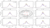 |
Fig. A.15. Same as Fig. A.13, but for TF. |
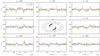 |
Fig. A.16. Same as Fig. A.1, but for spiral model. |
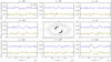 |
Fig. A.17. Same as Fig. A.16, but for PO. |
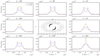 |
Fig. A.18. Same as Fig. A.16, but for TF. |
Spiral. The results for this model are shown in Figs. A.16–A.18. The φ-profiles are shown in Fig. A.16. This model is unique in having double-peaked φ-profiles when viewed from all azimuthal angles, similar to those found for distant and contact models, but with lower amplitude. The PO is shown in Fig. A.17. It shows a profile common for the single SMBH scenario for ϕ = 18°, 126°, 126°, and 342°, but also those with maximum PO in the core when viewed for all the other azimuthal viewing angles. The TF is shown in Fig. A.18. For intermediate inclination, it shows clear double-peaked profiles, while for nearly face-on viewing inclinations, a single-peaked profile or profiles with peaks very close to each other can be seen when ϕ = 18°, 198°, and 342°.
All Tables
All Figures
|
Fig. 1. Geometry and kinematics of the SMBBH for each model. From top to bottom panels: distant, contact, and mixed. Black arrows show the non-perturbed velocity field, while red ones are for clumps with an additional random component of the velocity. |
| In the text | |
|
Fig. 2. Distant model with mass ratio q = 0.5 (upper panel) and with q = 0.1 (lower panel). The black cross shows the center of mass, while the blue asterisk marks the L1 Lagrangian point. The color bar denotes the vertical offset from the xy plane. |
| In the text | |
|
Fig. 3. SMBBHs (black circles) with spiral arms surrounded by a CB disk. Each spiral is modeled with 500 clumps. The CB is modeled with 1000 clumps. The color bar denotes the vertical offset from the xy plane. |
| In the text | |
|
Fig. 4. Cartoon illustrating equatorial scattering region. The left figure shows the face-on view, while on the right the same geometry is shown when viewed edge-on. An example is shown for the case in which the two BLRs are separated. The BLRs are shown in yellow. The scattering region is shown in gray. |
| In the text | |
|
Fig. 5. Left panel: illustration of the model with a single SMBH in the center surrounded by a BLR (yellow) and the scattering region (gray) is shown. Right panel: profiles of polarization angle (top panel), the degree polarization (middle panel), and the total flux (bottom panel) when viewed from two intermediate inclinations. The polarization angle is given in degrees (°). We point out that the degree of polarization is given as fraction units and is lower than the ones we obtain in the following section due to the different size and optical depth of the scattering region. The total flux is given in arbitrary units. Model parameters are the same as the ones given by Savić et al. (2018). |
| In the text | |
|
Fig. 6. Left panels: illustration of each model with SMBBH in the center: Distant (panel a), contact (panel b), mixed (panel c), and spiral (panel d). Right panels, from top to bottom: φ, PO, and TF for two viewing inclinations and for azimuthal viewing angle ϕ = 18°. |
| In the text | |
|
Fig. A.1. Simulated profiles of φ across the line profile for two viewing inclinations i when observed from different azimuthal angles ϕ. Geometry and kinematics of the model are in the center for clarity. |
| In the text | |
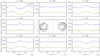 |
Fig. A.2. Same as Fig. A.1, but for PO. |
| In the text | |
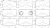 |
Fig. A.3. Same as Fig. A.1, but for TF. |
| In the text | |
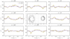 |
Fig. A.4. Same as Fig. A.1, but for q = 0.5. |
| In the text | |
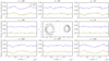 |
Fig. A.5. Same as Fig. A.2, but for q = 0.5. |
| In the text | |
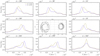 |
Fig. A.6. Same as Fig. A.3, but for q = 0.5. |
| In the text | |
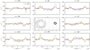 |
Fig. A.7. Same as Fig. A.1, but for q = 0.1. |
| In the text | |
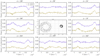 |
Fig. A.8. Same as Fig. A.2, but for q = 0.1. |
| In the text | |
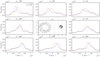 |
Fig. A.9. Same as Fig. A.3, but for q = 0.1. |
| In the text | |
|
Fig. A.10. Same as Fig. A.1, but for contact model. |
| In the text | |
|
Fig. A.11. Same as Fig. A.10, but for PO. |
| In the text | |
|
Fig. A.12. Same as Fig. A.10, but for TF. |
| In the text | |
|
Fig. A.13. Same as Fig. A.1, but for mixed model. |
| In the text | |
|
Fig. A.14. Same as Fig. A.13, but for PO. |
| In the text | |
|
Fig. A.15. Same as Fig. A.13, but for TF. |
| In the text | |
|
Fig. A.16. Same as Fig. A.1, but for spiral model. |
| In the text | |
|
Fig. A.17. Same as Fig. A.16, but for PO. |
| In the text | |
|
Fig. A.18. Same as Fig. A.16, but for TF. |
| In the text | |
Current usage metrics show cumulative count of Article Views (full-text article views including HTML views, PDF and ePub downloads, according to the available data) and Abstracts Views on Vision4Press platform.
Data correspond to usage on the plateform after 2015. The current usage metrics is available 48-96 hours after online publication and is updated daily on week days.
Initial download of the metrics may take a while.