| Issue |
A&A
Volume 623, March 2019
|
|
|---|---|---|
| Article Number | A60 | |
| Number of page(s) | 16 | |
| Section | Galactic structure, stellar clusters and populations | |
| DOI | https://doi.org/10.1051/0004-6361/201834188 | |
| Published online | 05 March 2019 | |
Galactic Archaeology with asteroseismic ages: Evidence for delayed gas infall in the formation of the Milky Way disc
1
Stellar Astrophysics Centre, Department of Physics and Astronomy, Aarhus University, Ny Munkegade 120, 8000 Aarhus C, Denmark
e-mail: This email address is being protected from spambots. You need JavaScript enabled to view it.
2
Dipartimento di Fisica, Sezione di Astronomia, Università di Trieste, Via G.B. Tiepolo 11, 34131 Trieste, Italy
3
I.N.A.F. – Osservatorio Astronomico di Trieste, Via G.B. Tiepolo 11, 34131 Trieste, Italy
4
I.N.F.N. – Sezione di Trieste, Via Valerio 2, 34100 Trieste, Italy
5
I.N.A.F. – Osservatorio Astronomico di Bologna, Via Gobetti 93/3, 40129 Bologna, Italy
Received:
4
September
2018
Accepted:
28
January
2019
Abstract
Context. Precise stellar ages from asteroseismology have become available and can help to set stronger constraints on the evolution of the Galactic disc components. Recently, asteroseismology has confirmed a clear age difference in the solar annulus between two distinct sequences in the [α/Fe] versus [Fe/H] abundance ratios relation: the high-α and low-α stellar populations.
Aims. We aim to reproduce these new data with chemical evolution models including different assumptions for the history and number of accretion events.
Methods. We tested two different approaches: a revised version of the “two-infall” model where the high-α phase forms by a fast gas accretion episode and the low-α sequence follows later from a slower gas infall rate, and the parallel formation scenario where the two disc sequences form coevally and independently.
Results. The revised two-infall model including uncertainties in age and metallicity is capable of reproducing: i) the [α/Fe] versus [Fe/H] abundance relation at different Galactic epochs, ii) the age−metallicity relation and the time evolution [α/Fe]; iii) the age distribution of the high-α and low-α stellar populations, iv) the metallicity distribution function. The parallel approach is not capable of properly reproducing the stellar age distribution, in particular at old ages.
Conclusions. The best chemical evolution model is the revised two-infall one, where a consistent delay of ∼4.3 Gyr in the beginning of the second gas accretion episode is a crucial assumption to reproduce stellar abundances and ages.
Key words: Galaxy: abundances / Galaxy: evolution / ISM: general / asteroseismology
© ESO 2019
1. Introduction
The main goal of Galactic Archaeology is to find and interpret signatures for the formation and evolution of our Galaxy from the observed chemical abundances and kinematics of resolved stellar populations (Bland-Hawthorn & Gerhard 2016). Tracing the history of the formation and evolution of our Galaxy is a fundamental step to understand the evolution of the Universe.
Each stellar atmosphere carries the enrichment history of the interstellar medium (ISM) from which it was formed. Once a star is born, and although its interior composition evolves, its atmosphere is negligibly polluted by the effects of stellar evolution. For this reason, stars are the surviving relics of formation and accretion episodes, and carry the most genuine signature of the processes that determined the formation and regulated the evolution of the various components of our Galaxy.
Chemical abundances are now routinely measured in stars belonging to the Galactic disc by spectroscopic surveys such as the Apache Point Observatory Galactic Evolution Experiment project (APOGEE, Majewski et al. 2017), the Gaia-ESO survey (Gilmore et al. 2012), and Galactic Archaeology with HERMES (GALAH, Buder et al. 2019) which makes use of the High-Efficiency and high-Resolution Mercator Echelle Spectrograph (HERMES) at the Anglo-Australian Telescope. Combining this wealth of information with kinematic properties of stellar “fossil” relics provided by the second Gaia data release (DR2, Gaia Collaboration 2018) offers an unparalleled opportunity to test galaxy formation models. This synergy has the potential to set strong constraints on the history of star formation and unravel the importance of the various physical processes that led to the formation of our Galaxy.
Previous works accomplished the determination of stellar ages based purely on spectroscopic or photometric information but for a limited number of stars in the solar vicinity: the Bensby et al. (2014) data sample is composed of 714 stars, that of Bergemann et al. (2014) of 144 stars, and the Haywood et al. (2013) sample is composed of 363 stars. Due to the difficulties in determining ages for field stars based purely on spectroscopic or photometric information, most studies of the Milky Way disc have focused on identifying different populations in the solar neighbourhood using chemistry and kinematics tagging. Recent data from spectroscopy pointed out the existence of a clear distinction between two sequences of disc stars in the [α/Fe] versus [Fe/H] space, for example the Gaia ESO Survey (Recio-Blanco et al. 2014; Rojas-Arriagada et al. 2016, 2017), the APOGEE project (Nidever et al. 2014; Hayden et al. 2015), and the the Archéologie avec Matisse Basée sur les aRchives de l’ESO (AMBRE) project (Mikolaitis et al. 2017). These sequences have been reproduced by tuning different parameters in chemical evolution models (e.g. Nidever et al. 2014; Snaith et al. 2015; Haywood et al. 2016; Grisoni et al. 2018, 2017), and recently predicted in the context of cosmological zoom-in simulations of Milky-Way-type galaxies (Grand et al. 2018; Mackereth et al. 2018).
Different prescriptions can be used in the chemical evolution models to reproduce particular features in the spectroscopic data. For instance, Snaith et al. (2015) and Haywood et al. (2016) considered the Galaxy as a closed-box system assuming that the accretion gas episodes are concentrated in the early initial phase of Galactic evolution. Those model are characterised by a significant dip in star formation between the high-α and low-α stars. On the other hand, several authors have developed models with episodes of exponential infall of gas throughout Galactic history, such as Spitoni et al. (2014), Côté et al. (2017), Rybizki et al. (2017), and Prantzos et al. (2018). All these models share the common feature of reproducing the observed distribution of stars in chemical space, that is, the two sequences in the [α/Fe] versus [Fe/H] plane. However, they predict different star formation histories and thus different correlations of stellar properties with age.
A step further from the constraints provided by abundance ratios and kinematics of stars comes from the new dimension provided by asteroseismology: precise stellar ages. Detailed asteroseismic analysis is a powerful tool to probe stellar interiors, since the oscillation frequencies are closely related to the physical properties of stars via the density and sound speed profiles (see Aerts et al. 2010; Chaplin & Miglio 2013, and references therein). Since these quantities are closely linked to the stellar mass and evolutionary stage, they can deliver precise ages of stars by comparing their oscillation spectrum with the predictions of stellar models (e.g. Casagrande et al. 2014; Serenelli et al. 2017; Pinsonneault et al. 2018). For field red giants, asteroseismic age uncertainties are at the level of ∼25% (e.g. Casagrande et al. 2016; Anders et al. 2017; Silva Aguirre et al. 2018).
With the recently established synergy of asteroseismic observations and high-resolution spectroscopy surveys, it has become possible to determine stellar properties for thousands of red giants in different regions of the Galaxy. Combining atmospheric parameters from APOGEE with data from the Kepler satellite, Silva Aguirre et al. (2018, hereafter VSA18) found that the two distinct sequences in the [α/Fe] versus [Fe/H] abundance ratios plane are characterised by a clear age difference. The low-α sequence age distribution peaks at ∼2 Gyr, whereas the high-α one does so at ∼11 Gyr. This was the first confirmation using asteroseismology of the age gap between these chemically selected populations, as already pointed out by for example Fuhrmann (1998) using a very local (∼25 pc) but complete sample in the solar neighbourhood. This age gap still needs to be confirmed in other Galactic regions, and the advent of asteroseismology as a tool for Galactic archaeology appears as the most promising route to test this paradigm across the Milky Way (e.g. Miglio et al. 2013; Casagrande et al. 2014; Stello et al. 2015).
In this paper we test our chemical evolution models with the aim of reproducing the new data by Silva Aguirre et al. (2018). We discuss two different approaches to reproduce the high and low-α sequences: i) the two-infall approach and the ii) parallel one. In the latter, the various Galactic stellar components begin to form at the same time but evolve in parallel at different rates. On the other hand, the revised two-infall model by Grisoni et al. (2017) follows a sequential scenario: first the thick disc is formed by a gas infall episode, and later a totally independent gas accretion event creates the thin disc over longer timescales.
Our paper is organised as follows. In Sect. 2 we present the APOKASC (APOGEE+ Kepler Asteroseismology Science Consortium) sample by VSA18. In Sect. 3 we describe the details of our adopted chemical evolution model for the solar neighbourhood. Section 4 presents our results related to the best two-infall model, and in Sect. 5 the model results in which we take into account the observational errors for the age and metallicity estimates are drawn. In Sect. 6 we present our results varying the infall timescales of the different accretion episodes. In Sect. 7 the parallel chemical evolution model results are reported. Finally, our conclusions are drawn in Sect. 8.
2. APOKASC sample by Silva Aguirre et al. (2018)
Pinsonneault et al. (2014) presented the first APOKASC catalogue of spectroscopic and asteroseismic properties of 1916 red giants observed in the Kepler field. The updated APOKASC sample presented by VSA18 is composed of 1989 red giants, with stellar properties determined combining the photometric, spectroscopic, and asteroseismic observables in the BAyesian STellar Algorithm (BASTA, Silva Aguirre et al. 2015, 2017) framework.
They associated to this sample proper motions from the first DR of Gaia (Lindegren et al. 2016; Gaia Collaboration 2016) and the Fourth US Naval Observatory CCD Astrograph Catalog (UCAC-4) catalogue (Zacharias et al. 2013). A first pruning procedure was applied by retaining only stars with precise kinematic information available.
To ensure that the chosen sample was representative of the physical and kinematic characteristics of the true underlying population of red giants in that direction of the sky, a selection function was applied adopting the Casagrande et al. (2016) method. Briefly, they corrected for the selection of oscillating giants with available APOGEE spectra, and after for the target selection effects of the Kepler spacecraft as a function of distance. The final sample presented by VSA18 is composed of 1197 stars. Due to its large number of stars with available ages and correction for selection effects compared to other studies (Haywood et al. 2013; Bergemann et al. 2014; Bensby et al. 2014), the APOKASC sample is to be regarded as extremely valuable and particularly suited for chemical evolution studies.
In Fig. 1 the observed [α/Fe] versus [Fe/H] abundance ratios for the stars presented by VSA18 are reported. Here, it is assumed that α abundances are given by the sum of the individual Mg and Si abundances (Salaris et al. 2018). The figure shows the disc components selected on the basis of their chemical properties: the high-α stars have ages of ∼11 Gyr, while the low-α sequence peaks at ∼2 Gyr. For guidance, we also depict the resulting prediction of our fiducial chemical evolution model (see Sect. 3 for details).
 |
Fig. 1. Observed [α/Fe] versus [Fe/H] abundance ratios presented by VSA18, compared with our fiducial chemical evolution model (blue line) and the classical two-infall model (yellow line) (see Sect. 4). The purple filled circles are the observed “high-α” stars, whereas the green filled circles are the observed “low-α” stars. The black-purple and black-green contour lines enclose the observed high-α and low-α stars, respectively. |
In the sample that we use throughout this work, we have not taken into account the so-called “young α rich” (YαR) stars. Understanding the origin of these stars has been the subject of a number of recent studies and they have been attributed to stars migrated from the Galactic bar (Chiappini et al. 2015) as well as evolved blue stragglers (Martig et al. 2015; Chiappini et al. 2015; Yong et al. 2016; Jofré et al. 2016). In the former case, it is believed that these stars formed in reservoirs of almost inert gas close to the end of the Galactic bar, while the latter scenario proposes that the YαR stars are the product of mass transfer or stellar merger events.
In the next sections we want to present a chemical evolution model focused only on the solar neighbourhood stars. Our aim is to provide a simple and valid scenario capable of explaining the majority of the stars and the new stellar ages contraints as provided by asteroseismology.
3. Chemical evolution model for the solar neighbourhood
We concentrate our study on the evolution with time of the solar annulus, defined here by an annular ring 2 kpc wide centred at 8 kpc from the Galactic centre. Our chemical evolution model is capable of tracing the abundance change with time of several chemical species (H, D, He, Li, C, N, O, α-elements, Fe, Fe-peak elements, s- and r-process elements). We take into account detailed nucleosynthesis from low and intermediate mass stars, Type Ia supernovae (SNe) (originating from white dwarfs in binary systems) and Ib/c and II SNe (originating from core-collapse of massive stars). The contribution of Type Ia SNe was first introduced by Matteucci & Greggio (1986). Here, the rate is calculated by assuming the single-degenerate model for the progenitor of these SNe, namely a carbon-oxygen white dwarf (C-O WD) plus a red giant companion in a binary system, and is expressed as
![Mathematical equation: $$ \begin{aligned} R_{\rm SNeIa}=A_{\rm Ia}\int \limits ^{M_{\rm BM}}_{M_{\rm Bm}}\phi (M_{\rm B})\left[ \int \limits ^{0.5}_{\mu _{\rm m}}f({\,}\mu )\psi (t-\tau _{M_{2}})\mathrm{d}\mu \right] \mathrm{d}M_{\rm B}, \end{aligned} $$](/articles/aa/full_html/2019/03/aa34188-18/aa34188-18-eq1.gif) (1)
(1)
where M2 is the mass of the secondary, MB is the total mass of the binary system, μ = M2/MB, μm = max[M2(t)/MB,(MB−0.5MBM)/MB], MBm = 3 M⊙, MBM = 16 M⊙. The initial mass function (IMF) is represented by ϕ(MB) and refers to the total mass of the binary system for the computation of the Type Ia SN rate, f( μ) is the distribution function for the mass fraction of the secondary, and AIa is the fraction of systems in the appropriate mass range, which can give rise to Type Ia SN events. Details about the assumed parameter values can be found in Spitoni et al. (2009).
The star formation rate (SFR) is implemented with the Kennicutt (1998) law
 (2)
(2)
where ν is the star formation efficiency, σg is the surface gas density, and k is the gas surface exponent with an exponent k = 1.5. For the IMF we use that of Scalo (1986) (constant in time and space).
The temporal evolution of the surface density of a certain chemical element Σi(R, t) is given by the expression
 (3)
(3)
where Xi(R, t) is the abundance by mass of the element i, ℛi(R, t) is the returned fraction, and ℬi(R, t) is the infall rate term.
We assume that the Galaxy is an “open” system and forms by gas accretion episodes that follow an exponentially decreasing infall rate as a function of time. This fundamental assumption adopted in most of the detailed numerical chemical evolution models of our Galaxy (Chiappini et al. 1997; Romano et al. 2010; Spitoni et al. 2014; Grisoni et al. 2017) helps solving the G dwarf distribution problem. Moreover, Colavitti et al. (2008) showed that the two-infall model of Chiappini et al. (1997) is qualitatively in agreement with results of the second release of GAlaxies with Dark matter and Gas intEracT (GADGET2, Springel 2005) cosmological hydrodynamical simulations when the standard cosmological parameters from Wilkinson Microwave Anisotropy Probe (WMAP; Spergel et al. 2007) are assumed.
Although an important ingredient of the Nidever et al. (2014) chemical evolution model to reproduce the APOGEE data was the inclusion of Galactic winds proportional to the SFR coupled to a variable loading factor, in this paper we do not consider outflows. In fact, Melioli et al. (2008, 2009) and Spitoni et al. (2008, 2009), studying the Galactic fountains processes originated by the explosions of Type II SNe in OB associations, found that the ejected metals fall back close to the same Galactocentric region where they are delivered and thus do not modify significantly the chemical evolution of the disc as a whole. Therefore, we do not take into account events of gas outflows in our models.
3.1. Updated two-infall model for the high-α and low-α components formation
We present here the two-infall chemical evolution model designed to reproduce the high-α and low-α stars sequences presented by VSA18. The infall rate ℬi(t, i), to be inserted in the right side of Eq. (3) is
![Mathematical equation: $$ \begin{aligned} {\mathcal{B} }_i(t,i)=(X_i)_{\rm inf} \left[ c_1 \, e^{-t/ \tau _{D1}}+ c_2 \, e^{-(t-t_{\rm max})/ \tau _{D2}} \right], \end{aligned} $$](/articles/aa/full_html/2019/03/aa34188-18/aa34188-18-eq4.gif) (4)
(4)
where (Xi)inf is the abundance by mass of the element i of the infall gas that here is assumed to be primordial, while tmax is the time for the maximum infall on the second accretion episode, that is, it indicates the delay of the beginning of the second infall. The typical value assumed for tmax in previous two-infall models without constraints from stellar ages is ∼1 Gyr (Chiappini et al. 2001; Romano et al. 2010; Spitoni et al. 2009).
The quantity τD1 is the timescale for the creation of the high-α stars and τD2 is the timescale for the formation of the low-α disc phase. Finally, the coefficients c1 and c2 are obtained by imposing a fit to the observed current total surface mass density in the solar neighbourhood, adopting the relations
 (5)
(5)
 (6)
(6)
where Σtot1(tG) and Σtot2(tG) are the present day total surface mass density of the high-α and low-α phases, respectively. In this particular model, differently from Nidever et al. (2014), we do not consider Galactic winds, in fact in the presence of winds, Eqs. (5) and (6) need to be revised.
3.2. Parallel formation scenario
With the aim of reproducing the data from the AMBRE project in the solar neighbourhood, Grisoni et al. (2017) tested the possibility of abandoning a sequential scenario in favour of a picture in which thick disc and thin disc stars are described by two coeval and independent evolutionary phases. This scenario was suggested by the fact that AMBRE data seemed to form two parallel sequences in the [Mg/Fe] versus [Fe/H] abundance ratio relation. In this paper we consider this scenario in the light of the new observational data by VSA18, comparing the stellar ages predicted by the model with the one provided by asteroseismology.
Therefore we have to solve in this case two independent sets of integro-differential equations presented by Eq. (3) assuming two distinct infall episodes. The gas infall rates for the high-α and low-α sequences are, respectively,
 (7)
(7)
 (8)
(8)
The quantities cT and cD along with the parameters τT and τD have the same meaning as the parameters introduced in Eq. (4). The novelty introduced by Grisoni et al. (2017) with this scenario is the fact that the infall rates of the phases are totally disentangled and coeval.
3.3. Nucleosynthesis prescriptions
For the nucleosynthesis prescriptions of Fe, Mg, and Si we adopted those suggested by François et al. (2004), who found that the yields at solar metallicity of Type II SNe of Woosley & Weaver (1995) provide the best fit to the data (details related to the adopted observational data are in François et al. 2004). The authors artificially increased the yields of Mg from massive stars from Woosley & Weaver (1995) to reproduce the solar Mg abundance. Magnesium yields from stars in the range 11–20 M⊙ have been increased by a factor of seven whereas those from stars larger than 20 M⊙ are lower than predicted by Woosley & Weaver (1995) (a factor of two on average). No modifications are required for the yields of Fe, as computed for solar chemical composition. Concerning Si, only the yields of the very massive stars (M > 40 M⊙) should be increased by a factor of two. The complete grid of the modified Mg, Si, and Fe yields can be retrieved from Table 1 of François et al. (2004). François et al. (2004) showed that concerning the yields from Type Ia SNe, revisions in the theoretical yields by Iwamoto et al. (1999) are suggested for Mg; with the aim of preserving the observed pattern of [Mg/Fe] versus [Fe/H], they also needed to increase the Mg yields from Type Ia SNe by a factor of five. The prescription for single low to intermediate mass stars is from van den Hoek & Groenewegen (1997), for the case of the mass loss parameter, which varies with metallicity (see Chiappini et al. 2003, model5). The choice of such ad-hoc nucleosynthesis prescriptions is supported by the fact that stellar yields are still a relatively uncertain component of chemical evolution models (Romano et al. 2010). The set of yields used in this paper has been adopted in several works (Cescutti et al. 2007; Spitoni et al. 2009, 2015, 2017; Spitoni & Matteucci 2011; Mott et al. 2013), and turned out to be able to reproduce the main features of the solar neighbourhood.
4. Model results for the revised two-infall model
First, we show the results related to the revised two-infall model considering the new constraints provided by the stellar ages computed with asteroseismology in terms of the [α/Fe] versus [Fe/H] abundance ratios. We recall that with α, here we mean the sum of the abundances of Mg and Si. We have adopted the photospheric values of Asplund et al. (2005) as our solar reference to be consistent with the APOGEE data release (García Pérez et al. 2016).
We tested several values for the input parameters of the chemical evolution model, and retained the combination that provided the best fit on chemistry and age to the observations reported by VSA18. The parameters included in this model are the following: the first infall is characterised by a current total surface mass density of 8 M⊙ pc−2 (Σtot1(tG) in Eq. (5)) and an infall timescale of τD1 = 0.1 Gyr. The second infall corresponds to a current total surface mass density of 64 M⊙ pc−2 (Σtot2(tG) in Eq. (6)) with an infall timescale of τD2 = 8 Gyr, and occurs after a delay of tmax = 4.3 Gyr. The star formation efficiency (SFE) is fixed at the value of ν = 1.3 Gyr−1. The total surface density for the low-α sequence is in agreement with the range of 54 and 74 M⊙ pc−2 for the thin disc given by Nesti & Salucci (2013, and references therein). For the thick disc surface mass density, the value suggested by Nesti & Salucci (2013) is approximately one tenth of that for the thin disc. In our model we assumed values consistent with this ratio (the ratio of total mass surface densities of high-α and low-α is 0.125).
In Fig. 1 we compare our best chemical evolution model with the VSA18 data in the [α/Fe] versus [Fe/H] plane, where an excellent agreement between the two is clearly seen. This level of agreement is only achieved if the second episode of gas infall (related to the low-α sequence) begins when the model curve of the first infall already covers the region populated by some of the stars from the low-α sequence. For this reason, we assume a slightly larger total surface mass density for the high-α component (8 M⊙ pc−2 than the 6.5 M⊙ pc−2 adopted by Grisoni et al. 2017), and require a delay time of tmax = 4.3 Gyr for the start of the second episode of gas infall. The sum of the high-α and low-α surface mass densities in our model, however, is very similar to the one of thick and thin disc components of Grisoni et al. (2017). In Fig. 1 we also show a model with the same parameters as in our fiducial one but with a delay time of tmax = 1.3 Gyr, hence similar to the one adopted in the “classical” two infall models (i.e. Chiappini et al. 1997; Spitoni et al. 2009; Grisoni et al. 2017). It is clear that the high-α stars are not reproduced. Here we can conclude that the usual delay adopted by the classical two infall model does not properly apply to the new VSA18 stellar sample. In Fig. 2 we present the α versus [Fe/H] plane colour coded by density of stars, and we labelled the ages of the stars created during the chemical evolution model curve. The densest regions are, as expected, also the regions where our model spends most of the time during its evolution (for roughly 10 Gyr the Galactic disc model is confined to the low-α evolutionary sequence). Different timescales of accretion are motivated by the fact that at early times the Galaxy assembled very quickly and efficiently, while at later times the formation of the Milky Way proceeded on much longer timescales as a consequence of dissipative collapse effects (Larson 1976; Cole et al. 2000).
 |
Fig. 2. Observed density of stars in the [α/Fe] versus [Fe/H] space for the APOKASC stars by VSA18, compared with our chemical evolution model (black solid line) in the solar neighbourhood. Filled red circles indicate the abundance ratios of the chemical evolution model at the given age. The area of each bin is fixed at the value of (0.083 dex) × (0.02 dex). |
In the title of this section we defined our two-infall model as a “revised” one. The novelty of our model compared to the classical two-infall model by Chiappini et al. (1997) and Spitoni et al. (2016, 2018) is the long delay before the starting of the second infall of gas.
In Fig. 2 the dilution effect caused by the second infall of primordial gas can be appreciated. Contrary to previous models (e.g. those of François et al. 2004; Cescutti et al. 2007; Romano et al. 2010; Grisoni et al. 2017), the delay of tmax = 4.3 Gyr in the peak of the second infall produces the nearly horizontal stripe at nearly constant [α/Fe] from [Fe/H] ≃ 0.35 dex to [Fe/H] ≃ −0.2 dex. The late accretion of pristine gas has the effect of decreasing the metallicity of each stellar population born immediately after the infall event, and has little effect on the [α/Fe] ratio since both α and Fe are diluted by the same amount.
When star formation resumes, Type II SNe produce a steep rise in the [α/Fe] ratio, which is then decreased and shifted towards higher metallicities due to pollution from Type Ia SNe. This sequence produces a loop in the [α/Fe] versus [Fe/H] plane of the chemical evolution track, which nicely overlaps with the region spanned by the observed low-α population. In our picture the observed “high-α” sequence can be explained in terms of our first infall phase, whereas the “low-α” is reproduced by the second gas infall.
A long delay between the gas infall episodes has been reported in simulations of late-type galaxies within a cosmological framework. For instance, Calura & Menci (2009) investigated the chemical properties of Milky-Way-like galaxies using a semi-analytical model within the hierarchical picture of galaxy formation and predicted the presence of an horizontal stripe in the [O/Fe] versus [Fe/H] plane caused by the presence of a substantial increment of late infall episodes. Moreover, Grand et al. (2018) studied the stellar disc properties of different Milky-Way-sized haloes extracted from very high resolution cosmological zoom-in AURIGA simulations. They found that a bimodal distribution in the [α/Fe] versus [Fe/H] plane is present when an early high-[α/Fe] star formation phase in the disc is followed by a shrinking of the gas disc. This shrinking is caused by a temporarily significant lowered gas accretion rate at ages between 6–9 Gyr, after which disc growth resumes through the occurrence of another infall episode. In our two-infall model, a lowering of the gas accretion is mimicked by a consistent delay in the second infall of gas.
A late time second accretion phase in a two-infall context has been also derived by Noguchi (2018) using the “cold flow” model by Dekel & Birnboim (2006) for cold-flows/shock heating. The Milky Way has been simulated using a code that divides the Galactic disc into a series of concentric annuli and the growth of the virial mass of the dark matter halo follows cosmological numerical simulations by Wechsler et al. (2002).
A first infall episode originates the high-α sequence, which is followed by a hiatus of 2 Gyr until the shock-heated gas in the Galactic dark matter halo has radiatively cooled and can accrete onto the Galaxy. The low-α sequence stars form during a second phase, after the hiatus. In agreement with our model, the SFR is characterised by two peaks, and in Noguchi (2018) they are separated by around five billion years. However, the pause in gas infall in Noguchi (2018) is present at later times than the one presented here, due to the fact that the author did not use the constraint from stellar ages to locate the infall hiatus as done in our analysis.
In Table 1, the solar abundances of Fe, Mg, and Si predicted by our two-infall model are compared with observations. The model solar abundances are determined from the composition of the ISM at the time of the formation of the Sun (after 9.5 Gyr from the Big Bang). It is evident that our model is able to reproduce the solar abundance ratios for the elements considered in this work. We have also tested whether our model is capable of reproducing the trends in Mg and Si provided by other observational studies and surveys. To this end, in Fig. 3 we compare the [Mg/Fe] and [Si/Fe] versus [Fe/H] predicted by our model in the solar neighbourhood with the data reported by Bensby et al. (2014). We find that our model reproduces satisfactorily the data.
Theoretical and observed solar abundances.
 |
Fig. 3. Comparison of our updated two-infall model with the observational data for thin and thick disc stars presented by Bensby et al. (2014). Upper panel: [Si/Fe] versus [Fe/H]. Lower panel: [Mg/Fe] versus [Fe/H]. Further details can be found in the text. |
An important constraint is represented by the present-time SFR in the solar vicinity. The upper panel of Fig. 4 shows the time evolution of the SFR in our model, which predicts a present day SFR value of 2.60 M⊙ pc−2 Gyr−1. This is in excellent agreement with the measured range in the solar vicinity of 2–5 M⊙ pc−2 Gyr−1 as suggested by Matteucci (2012) and Prantzos et al. (2018).
 |
Fig. 4. Upper panel: SFR time evolution predicted by the two-infall model for the solar neighbourhood. Lower panel: time evolution of the Type Ia SN (blue) and Type II SN (red) rates predicted by the two-infall model for the whole Galactic disc. |
By adopting a closed-box chemical evolution model, in Snaith et al. (2015) and Haywood et al. (2016) the SFR has been selected ad-hoc in order to reproduce the solar neighbourhood chemical data by Adibekyan et al. (2012) and Haywood et al. (2013). This different methodology compared to the two-infall approach leads roughly to the same transition time between the two α sequences, supporting our results and the robustness of the updated two-infall model.
The time evolution of the Type Ia SN and Type II SN rates is plotted in the lower panel of Fig. 4. The present day Type II SN rate in the whole Galactic disc predicted by our model is 1.31/[100 yr], in good agreement with the observations by Li et al. (2011), which yield a value of 1.54 ± 0.32/[100 yr]. The predicted present day Type Ia SN rate in the whole Galactic disc is 0.33/[100 yr], slightly below the observations by Li et al. (2011), which yield 0.54 ± 0.12/[100 yr], but in excellent agreement with the value provided by Cappellaro & Turatto (1997) of 0.30 ± 0.20/[100 yr].
In the VSA18 sample, the metallicity [M/H] is computed using the expression introduced by Salaris et al. (1993),
![Mathematical equation: $$ \begin{aligned} {\mathrm{[M/H]} } = {\mathrm{[Fe/H]} } (t) + \log \left(0.638 \times 10^\mathrm{[\alpha /Fe]}+0.362 \right). \end{aligned} $$](/articles/aa/full_html/2019/03/aa34188-18/aa34188-18-eq9.gif) (9)
(9)
We combined the abundance ratios [Fe/H] and [α/Fe] predicted by our model using this formulation to be consistent with the data. In Fig. 5 the results of the time evolution of the metallicity [M/H] and the [α/Fe] ratios are reported. Also here the effect of the dilution is evident, which produces a drop in the [M/H] when the second infall takes place. The general trend of the data is reproduced, however the VSA18 sample does not seem to show this kind of “knee” feature at an age of ∼9.6 Gyr.
 |
Fig. 5. Time evolution of [M/H] (upper panel) and [α/Fe] (lower panel) ratios for the stellar sample presented by VSA18, compared with our chemical evolution model predictions (black solid line). Purple filled circles depict the high-α population, whereas green filled circles represent the low-α one. In the upper panel, light blue symbols indicate median age uncertainties for 3 and 11 Gyr old stars of the VSA18 sample. |
In the lower panel of Fig. 5 the time evolution of [α/Fe] is presented. When the second infall begins, a sudden increase of [α/Fe] is predicted by our model as a result of the accretion of new primordial gas: Type II SNe (which trace the SFR) can pollute the ISM with α elements on short timescales, while Type Ia SNe need longer timescales to substantially pollute the ISM with Fe. The expected decrease in the [α/Fe] abundance is seen ∼2 Gyr after the second infall.
In conclusion, our revised two-infall model can reproduce the main features presented in the VSA18 dataset. The sudden drop in [M/H] and increase in [α/Fe] associated with the second accretion episode are not obvious in the observations but could be hidden behind the observational uncertainties. In the next section we will present the two-infall model results taking into account the error estimates related to stellar ages and metallicity.
5. Model results taking into account the observational errors
In Fig. 6 we report the average errors in bins of 0.5 Gyr as a function of the Galactic age for the estimated stellar ages for the APOKASC sample by VSA18. We note that the errors in the stellar age determination are strongly dependent on the Galactic age, and span a huge range of values: between σAge = 0.13 Gyr (at the Galactic age of 0.25 Gyr) and σAge = 4.93 Gyr (at a Galactic age of 14 Gyr). On the other hand, the errors on the abundance ratio [M/H] reported by APOGEE are independent from the stellar ages and the average value is σ[M/H] ∼ 0.118 dex.
 |
Fig. 6. Observed error estimate on the stellar ages for the whole data sample (both low-α and high-α stars) by VSA18 (blue circles). The red line is the average observed error estimate on age bins of 0.5 Gyr. |
We take into account these errors in our model by adding, at each Galactic time, a random error to the ages and metallicities [M/H] of the stellar populations formed at Galactic time t. These random errors are uniformly distributed in the interval described by the average errors estimated at that time (see solid red line in Fig. 6), and we define the “new age” including these uncertainties as
![Mathematical equation: $$ \begin{aligned} {\mathrm{Age} }_{\rm new}(t) = {\mathrm{Age} } (t) + U([-\sigma _{\rm Age}(t), \sigma _{\rm Age}(t) ]), \end{aligned} $$](/articles/aa/full_html/2019/03/aa34188-18/aa34188-18-eq10.gif) (10)
(10)
where Age (t) = (13.7 − t) Gyr, and U is the random generator function. Similarly, we implement the error in the chemical abundance space through the relation
![Mathematical equation: $$ \begin{aligned}[{\mathrm{M/H} }]_{\rm new}(t) = [{\mathrm{M/H} }](t)+ U([-\sigma _{\rm [M/H]}(t), \sigma _{\rm [M/H]}(t) ]). \end{aligned} $$](/articles/aa/full_html/2019/03/aa34188-18/aa34188-18-eq11.gif) (11)
(11)
In Fig. 7 the results of the metallicity time evolution [M/H] and the [α/Fe] ratios including the errors described in Eqs. (10) and (11) are reported.
 |
Fig. 7. Chemical evolution model results for the time evolution of [M/H] (upper panel) and [α/Fe] (lower panel) distributions produced from the age and metallicity uncertainties reported by VSA18 following Eqs. (10) and (11). With the purple filled pentagons we label the stellar populations formed during the first infall (“high-α” sequence) at Galactic time t < tmax = 4.3 Gyr (time for the maximum infall on the second gas infall) before including the errors. Analogously, the filled pentagons green circles represent the stellar populations formed in “low-α” sequence at Galactic time t > tmax = 4.3 Gyr. The pentagon size indicates the local number density of formed stars normalised to maximum value. We also show the contour density curves of the observed “high-α” stars (black and blue lines stand for the higher and lower levels, respectively) and “low-α” stars (black and white lines stand for the higher and lower levels, respectively) of the VSA18 sample. |
In the remainder of the paper we will refer to our chemical evolution model combined with the observational errors as to our synthetic model. Comparing our model results with the data, we see that they effectively reproduce the observational trends, and our synthetic model results do not show the “knee-like” feature in the [M/H] and [α/Fe] associated with the second gas infall episode (in contrast to the model curves in the two upper panels of the same figure). The inclusion of the error in the stellar ages and metallicites allows our model to also predict a presence component of old (t > 10 Gyr) low-α stars that are observed in the dataset. Moreover it can be seen that, in the [α/Fe] versus age plot, the observed spread of the oldest high-α stars is comparable with that of the model.
Our “simple” scenario is able to explain the general trends of the APOKASC sample. We underline that the sample presented by VSA18 selected stars with a [M/H] > −1 dex, and therefore we show only predicted stars above this threshold for [M/H]. With variable symbol size we also indicate the density of the local number of formed stars predicted by our synthetic model normalised to its maximum number. In the upper panel of Fig. 7 we see that some of the high-α stars predicted by our synthetic model show larger [M/H] values than the observed ones (purple pentagons outside the blue contour lines). These stars appear in the lower panel of Fig. 7 at ages older than 6 Gyr and [α/Fe] abundance ratios smaller than 0.05 dex, not seen in the VSA18 observations. However, the number density of these high-α stars is negligible compared to the density of low-α stars formed at the same age. In conclusion, there is no tension between our synthetic model results and the VSA18 sample. We notice that our synthetic high-α stars present less spread than the observed one, and stellar migration from outer Galactic regions could be a possible explanation for this discrepancy (Schönrich & Binney 2009).
VSA18 claimed that the majority of the observed high-α stars have ages in the range of ∼8 to ∼14 Gyr and show no tight correlation between age and [α/Fe]. Our synthetic model for the high-α sequence is in agreement with this statement. In fact, the region with higher predicted stellar density is above [α/Fe] = 0.05 dex, and the inclusion of observational errors washes away the visible tight correlation in the chemical evolution results. Rojas-Arriagada et al. (2016) claimed that the formation of the high-α and low-α sequences is not strictly sequential but they partly overlap in time. This fact would imply that the two sequences are not entirely sequential as noted in Haywood et al. (2013) and Noguchi (2018). On the other hand, the inclusion of observational errors in our synthetic model creates in the age-metallicity and in the age-[α/Fe] a partial overlapping of the two stellar sequences as visible in Fig. 7.
In Fig. 8 we compare our model results with the inclusion of errors with the observational data in the classical chemical evolution plot [α/Fe] versus [Fe/H] for different stellar ages. Overall, it is clearly shown how our synthetic model including observational errors adopting Eqs. (10) and (11) fits the data extremely well. The upper left panel shows the stars in the VSA18 sample with ages older than 11 Gyr. It is also evident that the oldest stars seem to confirm our astroarcheology scenario: they keep the signature of the delayed infall of gas and the successive dilution effect on the [α/Fe] versus [Fe/H] relation as shown by the horizontal stripe at roughly constant [α/Fe]. However, stars considered here are older than 11 Gyr, whereas our delayed infall starts 4.3 Gyr after the Big Bang (corresponding to a Galactic age of 9.4 Gyr). When taking into account the observational errors in our synthetic model, stars born shortly after the second infall episode have corresponding age uncertainties large enough to make them consistent with ages older than 11 Gyr (cf., Fig 6). Thus, our model suggests that the population of old low-α stars is an artefact created by large errors in the ages of stars older than ∼8 Gyr.
 |
Fig. 8. Abundance ratios of [α/Fe] as a function of [Fe/H] predicted by our two-infall chemical evolution model (cyan circles) taking into account the average observational errors on age and metallicity (following Eqs. (10) and (11)) computed for different age ranges. Also plotted are the observational data, colour coded as in Fig. 1. Upper left panel: stars older than 11 Gyr. Upper right panel: stars formed throughout the Galactic history. Lower left panel: stars younger than 8 Gyr. Lower right panel: stars younger than 4 Gyr. |
In the upper right panel all stars of the sample are compared with our model, showing that very good agreement between data and model prediction is clearly achieved. The lower left panel presents ages younger than 8 Gyr, and we note that the bulk of stars predicted by our model belong to the low-α sequence and only a small fraction present high-α values. The data shows a small number of stars in the high-α sequence at metallicities below [Fe/H] ≃ −0.3 not predicted by our model, but the overall agreement is good. Finally, the lower right panel shows the case of stars younger than 4 Gyr. Almost all the observed stars belong to the low-α sequence and occupy a metallicity range larger than that predicted by our model. However, the region between −0.2 dex < [Fe/H] < 0.3 dex where synthetic results are located corresponds to the area with the highest number of observed stars.
The value of tmax has been tuned by imposing that our synthetic model should be able to reproduce the observed stars older than 11 Gyr (upper left of Fig. 8) in the [α/Fe] versus [Fe/H] relation. Including the observational error, our “best model” should predict the horizontal stripe that characterises low-α sequence stars older than 11 Gyr.
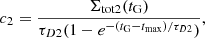
We recall that in this work we adopt for the high-α sequence the same infall timescale as the thick disc phase of Grisoni et al. (2017), τD1 = 0.1 Gyr. With this particular value, Grisoni et al. (2017) successfully reproduced the metallicity distribution function (MDF) of the thick disc stars of the AMBRE project. Figure 1 shows that the high-α sequence stars in the [α/Fe] versus [Fe/H] relation of the VSA18 sample are also well reproduced with τD1 = 0.1 Gyr: the model line passes through the higher density peaks indicated by the contour plot curves. In the upper panel of Fig. 9, we explore different tmax values spanning the range between 1.3 and 4.3 Gyr, assuming τD1 = 0.1 Gyr. It is clear that already a delay tmax 1 Gyr shorter than the one adopted in this work will not allow us to reproduce the data. In the lower panel of Fig. 9, we show the predicted [α/Fe] versus [Fe/H] abundance ratios by the synthetic model for stars older than 11 Gyr with τD1 = 0.1 Gyr, τD2 = 8 Gyr, and τmax = 3.3 Gyr. The horizontal stripe is located at a much higher [α/Fe] value than the one shown by low-α data.
 |
Fig. 9. Upper panel: effects on the chemical evolution of the solar neighbourhood in the [α/Fe] versus [Fe/H] abundance ratios of different values for the delay of the beginning of the second infall (the quantity tmax in Eq. (4)). Lower panel: [α/Fe] abundance ratios as a function of [Fe/H] predicted by our two-infall chemical evolution model (salmon circles) taking into account the average observational errors on age and metallicity (following Eqs. (10) and (11)) for stars older than 11 Gyr, considering a delay for the beginning of the second infall of tmax = 3.3 Gyr. Also plotted is the observational data, colour coded as in Fig. 1. |
We stress that the location of the horizontal stripe is independent of the choice of τD2. Naturally, different values of τD2 will lead to different loop sizes in the low-α sequence: smaller values will lead to more extended loops in the [α/Fe] versus [Fe/H] relation (see discussion in Sect. 6).
Finally, the value of τD2 has been tuned with the aim of:
-
reproducing 1) the present day SFR, 2) the present day Type Ia and Type II SN rates, 3) the solar abundances of Asplund et al. (2005);
-
covering the spread in chemical space of the low-α sequence with our synthetic model, which takes into account the observational errors (see upper right panel of Fig. 8);
-
reproducing the observed age distributions of the high-α and low-α sequences, and the MDF (see Figs. 10 and 11).
 |
Fig. 10. Upper panel: age distribution of stars formed during the whole Galactic history predicted by our two-infall chemical evolution models. Middle panel: age distribution of the observed high-α sequence stars of the VSA18 sample (purple histogram) compared to the predicted distribution of stars created during the first infall episode, and taking into account the errors given by Eqs. 10 and 11 (cyan histogram). Lower panel: age distribution of low-α stars in the VSA18 sample (green histogram) compared to the model-predicted distribution of stars created during the second infall episode, taking into account the errors given by Eqs. (10) and (11) (cyan histogram). |
 |
Fig. 11. Metallicity distribution predicted by our chemical evolution model indicated by the red histogram. The observed distribution calculated including both high-α and low-α stars is shown by the black, empty histogram. The cyan line indicates the metallicity distribution of our chemical evolution model convolved with a Gaussian with standard deviation σ = 0.13 dex. Finally, the purple line indicates the metallicity distribution of our chemical evolution model convolved with a Gaussian with standard deviation σ = 0.07 dex. |
In Fig. 9 we note that a delay of tmax = 1.3 Gyr at the beginning of the second gas accretion episode is similar to the one adopted in the classical two-infall chemical evolution model presented by Chiappini et al. (2001) and Spitoni et al. (2009). Small differences between the two-infall model presented in Fig. 9 with tmax = 1.3 Gyr and the classical ones are due to the adopted model prescriptions: in our model we did not consider a threshold in the SFR and the first infall timescale is shorter. Here we can conclude that the usual delay adopted by the classical two-infall model does not properly apply to the new VSA18 stellar sample. In Sect. 6 we will show how sensitive the chemical evolution results are to different choices for the infall timescales τD1 and τD2.
It is also worth noting that Hayden et al. (2015) presented the [α/Fe] versus [Fe/H] relation for APOGEE stars at different Galactocentric distances. The correspondence between our results reported in Fig. 8 for different stellar ages in the solar neighbourhood and the Hayden et al. (2015) results (see their Fig. 4) is evident. In fact, according to Hayden et al. (2015), stars preferentially populate the low-α sequence in the [α/Fe] versus [Fe/H] relation in the outer Galactic regions, which is in agreement with our results for stars younger than 4 Gyr. In the light of our results and in the presence of the stellar ages provided by asteroseismology, our analysis coupled with the observations presented by Hayden et al. (2015) confirms an inside-out formation scenario for the Galactic disc: outer Galactic regions have few old stars and show only recent episodes of star formation. Moreover, the Hayden et al. (2015) data show that in the outer regions the locus of the low-α sequence shifts towards lower metallicity. This can be well explained by inside-out formation: external Galactic regions are formed on longer timescales, hence the chemical enrichment is weaker and less efficient than the inner Galactic regions, leading to a smaller metallicity. As discussed in the Introduction, inside-out formation is well motivated by the dissipative collapse scenario (Larson 1976; Cole et al. 2000).
In Fig. 10 we report our model results in terms of the stellar age distribution. In the upper panel the distribution of stars formed during the whole Galactic history predicted by our two-infall chemical evolution models is drawn. The distinction between old stars, whose distribution peaks within the first Gyr of the Galactic time, and the young ones related to the second infall of gas is clearly shown. In order to compare our model results with the age distributions given by VSA18, we considered the errors introduced in Eqs. (10) and (11).
With the aim of comparing the observed high-α sequence with our model, we want to consider only the stars formed up to the time at which the second infall starts (i.e. Galactic time t < tmax = 4.3 Gyr). For this purpose, we convolved our stellar age distribution with mock observational errors to create a new stellar age distribution.
Moreover, to be consistent with the data, we considered only stars with [M/H] > −1 dex. In the middle panel of Fig. 10, we report this distribution along with the observed one. We note that the data are reasonably well reproduced, even if we predict more stars at the early times. The median of the observed high-α stellar ages distribution is  Gyr, whereas the one predicted by our synthetic model for the high-α sequence is
  Gyr.
Gyr.
In fact, in order to best match the [α/Fe] versus [Fe/H] abundance ratio, we have to consider a very fast evolution for the high-α stars. Anyway, including the observational age error, our model predicts a spread in the age distribution in agreement with the one suggested by the data.
Adopting the same method, the age distribution of the stars formed during the second infall of gas is compared with the APOKASC low-α sample in the middle plot of Fig. 10. The general data trend is reproduced, but some differences between model and observations can be noticed also in this case: the observations show a distribution peaked at slightly younger ages. In fact, the median of the observed low-α stellar ages distribution is  Gyr, whereas the one predicted by our synthetic model is
  Gyr.
Gyr.
In Fig. 11 the MDF of the two-infall model, without taking into account any kind of observational errors, is compared with the whole data sample (low-α + high-α stars). The MDF is expressed in terms of the abundance ratio [M/H] introduced in Eq. (9). It is evident that our model is consistent with the data but predicts less stars at super-solar metallicities compared to the data. The two distributions are normalised to the corresponding maximum number of stars for each distribution.
In the same figure we also show the curve related to the model distribution convolved with a Gaussian with a σ fixed at the value of 0.13 dex, consistent with observational errors. The model line with the convolution (normalised at the total number of stars) better reproduces the data, as shown by the cyan line in Fig. 11. The model results related to the case in which we convolved our MDF with a Gaussian with a σ0.07 dex is also shown. We recall that the average [M/H] error in APOGEE is ∼0.12 dex. We show results for two values of sigma: one slightly larger (σ = 0.13 dex) and another one smaller (σ = 0.07 dex) than the average observational error with the aim of showing how the distribution is affected by different σ values. In conclusion, this scenario is capable of reproducing almost all the observational proprieties. Contrary to Nidever et al. (2014), we do not need the superposition of several populations with different enrichment histories, or variable loading factor winds combined with different star formation efficiencies in time. Our scenario is simpler and it is in agreement with the stellar ages provided by asteroseismology.
In Fig. 12 we compare the age-metallicity and time evolution of the [α/Fe] abundance ratio of our updated two-infall model (without including errors) with the Bensby et al. (2014) data. Our model is consistent with the data given the large uncertainty in the stellar age determinations. Comparing the age errors of Fig. 12 with those of the asteroseismology in Fig. 6, it is clear that asteroseismology has opened a new era in Galactic Asteroarchaelogy. While our results are also consistent with the data by Bergemann et al. (2014), some discrepancy related to the high-α sequence emerges with the Haywood et al. (2013) data. In that paper the high-α stars show a tight relation in the age versus [α/Fe] in contrast with the finding by VSA18. Also our chemical evolution model predicts a tight correlation with a steeper slope; however, once we include the observational errors, this correlation disappears in the [α/Fe] versus age. As underlined above, regions with the higher density of high-α stars formed by our model (see lower panel of the Fig. 7) overlap with the VSA18 data (stars with ages between 8 and 14 Gyr and [α/Fe] larger than 0.05 dex).
 |
Fig. 12. Time evolution of [Fe/H] (left panel) and [α/Fe] (right panel) predicted by our chemical evolution model (black solid lines) compared with the observational values of the sample presented by Bensby et al. (2014). |
The discrepancy between Haywood et al. (2013) and VSA18 data could be due to the fact that Haywood et al. (2013) results are based on a sub-sample of Adibekyan et al. (2012) composed of only 363 stars with meaningful ages, corresponding to bright turn-off dwarfs (in Adibekyan et al. 2012 dwarfs are selected for exoplanet detection studies) where no assessment has been made of how representative they are of the underlaying population.
6. Testing different timescales of accretion τD1 and τD2
In this section we test the impact on the chemical evolution of the solar neighbourhood of varying the timescales of primordial infalling gas. Retaining the same model prescriptions of the best model presented in Sect. 4, in the upper panel of Fig. 13 we show the results of considering different values of τD1: 0.1, 0.5, 1, and 2 Gyr. It is evident that as chemical enrichment is faster and more efficient (i.e. as τD1 gets shorter):
-
the high-α disc phase is shifted towards larger [Fe/H] values;
-
the system presents a lower [α/Fe] value when the second infall starts (we recall that it takes place at tmax = 4.3 Gyr). This is due to the fact that Type II SNe trace the SFR. If the SFR peaks at an early time (e.g. τD1 = 0.1), at tmax = 4.3 Gyr the iron produced by Type Ia SNe with a time delay will dominate the ISM pollution (Matteucci et al. 2009; Bonaparte et al. 2013; Vincenzo et al. 2017). When the SFR is more extended in time (e.g. τD1 = 2), a smaller [α/Fe] abundance ratio is therefore expected.
In Fig. 14 we explore the age-metallicity (in terms of [M/H]) and age-α relations for models with different τD1 values (same values as in the upper panel of Fig. 13). Models with shorter infall timescales predict higher metallicities at the beginning of the second accretion phase (t = tmax = 4.3 Gyr), while the model with the longest timescale (τD1 = 2 Gyr) reaches the lowest metallicity after tmax before the pollution by Type II SNe resumes.
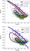 |
Fig. 13. Effects on the chemical evolution of the solar neighbourhood in the [α/Fe] versus [Fe/H] plane of different timescales for primordial gas infall. Upper panel: timescale variations for primordial gas accretion related to the high-α sequence (τD1). Lower panel: timescale variations for primordial gas accretion related to the low-α sequence (τD2). |
In the lower panel of Fig. 14 we show the same models in terms of the predicted time evolution of the abundance ratio [α/Fe]. At the moment of the start of the second infall (tmax = 4.3 Gyr after the Big Bang), models with shorter timescales of gas accretion τD1 have smaller SFR compared to models with longer timescales. Therefore, the Type II SN contribution is smaller, whereas the Fe produced by Type Ia SNe with a delay time distribution is important. Hence a smaller [α/Fe] is expected as shown in Fig. 14.
Always adopting the same model prescriptions of our best two-infall model (and τD1 = 0.1), in the lower panel of Fig. 13 we show the results when we vary the second infall timescale τD2 assuming the following values: τD2 = 2, 4, 8, and 9 Gyr. It is evident that the size of the “loop” is strongly dependent on the timescale of gas accretion τD2. In fact, at the beginning of the second accretion event, the infall rate of pristine gas is higher for smaller τD2 and therefore the dilution effect (longer horizontal excursion towards lower [Fe/H] values) is more evident. Consequently, a more extended loop in the [α/Fe] versus [Fe/H] relation appears as a result of the larger increase in [α/Fe] produced by Type II SNe for smaller τD2.
In Fig. 15 we show the age and α abundances evolution compared to our models calculated with different τD2 values (the same models as those shown in the lower panel of Fig. 13). In systems with shorter timescales of accretion τD2, the rate of gas accretion during the second infall is high at Galactic times t ≃ tmax, hence the dilution works efficiently. In fact, in the upper panel of Fig. 15 we see that the model with τD2 = 2 Gyr presents the deepest drop in the age versus [M/H] relation.
 |
Fig. 14. Time evolution of [M/H] (upper panel) and [α/Fe] (lower panel) shown for the VSA18 sample (same as Fig. 5) and our chemical evolution model with different timescale values for the first infall of gas (τD1) |
In the lower panel of Fig. 15, the model with the highest bump in the [α/Fe] abundance ratio is the one with the shortest timescale of accretion τD2. As briefly mentioned before, the star formation activity is tightly connected with the rate of Type II SNe, and hence to the α-element production. On the other hand, Fe production needs a certain time delay and this is the reason why the model curve with τD2 = 2 Gyr shows the steepest increase in the [α/Fe] soon after the beginning of the second infall.
7. Model results for the parallel formation scenario
Following the scenario proposed by Grisoni et al. (2017) we show here the results for the parallel model. We recall that in this scenario the high-α and low-α sequences evolve 1) independently 2) and coevally.
In Fig. 16 we show the results of a chemical evolution model in the [α/Fe] versus [Fe/H] plane. Following Eqs. (7) and (8), the timescales of gas accretion are τT = 0.1 Gyr and τD = 7 Gyr, assuming the same values adopted by Grisoni et al. (2017).
 |
Fig. 16. Model results of the parallel approach for the abundance ratios [α/Fe] versus [Fe/H]. We report the evolution of the high-α (solid line) and the low-α (dashed line) model sequences. Observational data are the same as in Fig. 1. |
The SFEs for the high-α and low-α sequences are fixed at the values of ν = 1.3 Gyr−1 and ν = 0.7 Gyr−1, respectively, and the current total surface mass densities are the same as those from our revised two-infall model. An overall good level of agreement is obtained between the data and the model: the high-α sequence is reproduced by a fast and efficient evolution, whereas the low-α stars are better characterised by a slower evolution (as shown by Grisoni et al. 2017).
However, this scenario presents several flaws in the light of the new key information as provided by asteroseismology: stellar ages. In fact, in Fig. 17 we present the age distribution of the low-α sequence predicted by our chemical evolution model, which also takes into account the observational errors described by Eqs. (10) and (11).
We notice that the age distribution of the stars formed in the low-α model is very different from the one presented by VSA18: too many stars in the parallel approach are created at early times, whereas the observed distribution shows that the majority of them have ages between between 2 and 4 Gyr. We recall that the median of the observed low-α age distribution is located at  Gyr, whereas the one predicted by our synthetic parallel model is
  Gyr.
Gyr.
On the other hand, in Fig. 18 we show that the age distribution predicted by the high-α sequence of the parallel approach is in agreement with the observational data. The median of the observed high-α age distribution is  Gyr, whereas the one predicted by our high-α synthetic parallel model sequence is
  Gyr.
Gyr.
 |
Fig. 17. Upper panel: stellar age distribution predicted by the parallel chemical evolution model for the low-α phase. Lower panel: age distribution for the low-α model sequence in which we have taken into account age and [M/H] errors (cyan histogram). Also plotted is the histogram of the age distribution for the low-α stars from VSA18 (green). |
These results are further analysed in Fig. 19, where we show the evolution of metallicity and [α/Fe] for the parallel model. The thin line in the high-α sequence represents the chemical evolution phase in which the number of stars formed in age bins of 1 Gyr is smaller than 2% of total number of stars created over the whole Galactic lifetime (the age distribution in the upper panel of Fig. 18 shows that it is true for Galactic ages smaller than ∼8 Gyr).
 |
Fig. 19. Panels a and b: same as Fig. 5 for the parallel model results. The dashed black line depicts the low-α model phase, whereas the black solid line stands for the high-α phase. In the latter case, the thin line shows the period of the evolution when the number of stars born in age bins of 1 Gyr is smaller than 2% of total number of stars formed. Panels c and d: chemical evolution model results where we have taken into account estimated age and [M/H] errors. Analogously to the thin solid line in the upper two panels, smaller purple starred symbols are associated to stars with ages lower than 8 Gyr (before the inclusion of age errors). Details are given in the text. |
We notice that the high-α sequence is characterised by a fast and efficient chemical enrichment, with high values of [M/H] compared to the low-α model. In the two lower panels of Fig. 19, the time evolution of metallicity [M/H] and [α/Fe] ratios including the errors described in Eqs. (10) and (11) are reported for the parallel model. The metallicity predicted by the model for the high-α sequence at young ages is much higher than the observed metallicity distribution of stars. However, given that the fraction of young stars formed in the high-α sequence is negligible compared to the old ones (cf. Fig. 18), these stars are unlikely to be observed.
Looking at the evolution of [α/Fe] predicted by the parallel model, we see significant differences compared to the observed distribution obtained from asteroseismology. In fact, at early times the low-α model predicts that the majority of the stars should have high [α/Fe] values. Moreover, the low-α sequence predicts at young ages stars with much lower [α/Fe] values than the ones observed.
A more evident tension between the observational data and the models is present in the [α/Fe] versus [Fe/H] plane for stars older than 11 Gyr, as shown in Fig. 20. After including the uncertainties in age and metallicity, the model cannot reproduce the population of stars at −0.5 < [Fe/H] < 0.25 and [α/Fe] ≤ 0.05. Even if this population of old low-α stars is misclassified due to large age uncertainties, the revised two-infall model was capable of predicting the existence of such objects once appropriate errors were included in the model calculations. In the parallel model there is the lack of an horizontal stripe in the [α/Fe] versus [Fe/H] plane, which characterises the observational data at different Galactic ages (see data in Fig. 8). We conclude that the purely parallel approach fails to reproduce the data in the solar neighbourhood if we take into account the new dimension provided by asteroseismology, the stellar age.
 |
Fig. 20. Abundance ratios of [α/Fe] as a function of [Fe/H] predicted by means of the parallel chemical evolution model including age and [M/H] errors for the high-α and low-α model phases (empty magenta and green pentagons, respectively). Both models and data are related to stars older than 11 Gyr. |
8. Conclusions
We have studied in detail chemical evolution models in the solar annulus with the aim of reproducing the new observational data by Silva Aguirre et al. (2018), concerning both chemical abundance ratios and precise stellar ages as provided by asteroseismology. Our main conclusions can be summarised as follows:
-
Our revised two-infall model in the solar neighbourhood reproduces well the observational stellar properties of both the high-α and low-α sequences;
-
The APOGEE data is consistent with the presence of a delayed second infall of gas, which in our model creates a loop in the [α/Fe] versus [Fe/H] plane that corresponds to low-α stars;
-
With the inclusion in our model of the observational age and metallicity uncertainties, we effectively reproduce i) the spread in the age-metallicity relation, and ii) the time evolution of the [α/Fe] abundance ratio. Moreover, the observed stars older than 11 Gyr seem to confirm our astroarcheology scenario. In fact, these stars keep the signature of a second infall of gas delayed by ∼4.3 Gyr with respect to the first episode and the successive dilution effect in the [α/Fe] versus [Fe/H] plane;
-
Our revised two-infall model results are in agreement with the observed age distribution of the stars of the high-α and low-α sequences, and with the observed metallicity distribution function;
-
We showed that the parallel model, in which the high-α and low-α sequences form coevally but independently with different timescales of accretion is not able to reproduce the constraints given by the stellar ages. In fact, the low-α sequence model cannot reproduce the location in the [α/Fe] versus [Fe/H] plane of stars older than 11 Gyr even when observational uncertainties are taken into account. Moreover, the low-α sequence predicts, at young ages, stars with much lower [α/Fe] values than the ones observed.
By means of chemical evolution models, we provide constraints on the accretion history of the Milky Way in the light of new observational data. We show that the two-infall model is still a valid one but we pointed out the importance of a consistent delay in the second accretion (tmax = 4.3 Gyr) to properly reproduce the properties of the low-α stars. The presence of an horizontal sequence in the [α/Fe]-[Fe/H] plane was predicted by Calura & Menci (2009) by means of chemical evolution models in a cosmological framework. A new assessment of such a feature by means of up-to-date galaxy formation models is to be considered for future work. Our results are consistent with very high-resolution cosmological zoom-in AURIGA simulations for Milky-Way-sized haloes presented by Grand et al. (2018). They found that a bimodal distribution in the [α/Fe] versus [Fe/H] plane is due to the presence of a temporarily lowered gas accretion rate. In our two-infall model a lowering of the gas accretion is mimicked by a consistent delay in the second infall of gas.
Nevertheless, the scenario presented in this work is not complete. In fact, we ignored in our analysis the YαR stars, which are believed to be initiated by an interacting binary stellar system or stellar migration. We did not discuss the effects of stellar migration, which plays an important role, but focused on providing a simple formation scenario still able to reproduce the new, tight constraints provided by the asteroseismic stellar ages. Further analysis including stellar kinematics will be the subject of an upcoming publication.
Acknowledgments
We thank the anonymous referee for various suggestions that improved the paper. E. Spitoni thanks K. Verma for helpful discussions. E. Spitoni and V. Silva Aguirre acknowledge support from the Independent Research Fund Denmark (Research grant 7027-00096B). V. Silva Aguirre acknowledges support from VILLUM FONDEN (Research Grant 10118). F. Matteucci acknowledges research funds from the University of Trieste (FRA2016). F. Calura acknowledges funding from the INAF PRIN-SKA 2017 programme 1.05.01.88.04.
References
- Adibekyan, V. Z., Sousa, S. G., Santos, N. C., et al. 2012, A&A, 545, A32 [NASA ADS] [CrossRef] [EDP Sciences] [Google Scholar]
- Aerts, C., Christensen-Dalsgaard, J., & Kurtz, D. W. 2010, Asteroseismology (New York: Springer) [Google Scholar]
- Anders, F., Chiappini, C., Rodrigues, T. S., et al. 2017, A&A, 597, A30 [NASA ADS] [CrossRef] [EDP Sciences] [Google Scholar]
- Asplund, M., Grevesse, N., & Sauval, A. J. 2005, in Cosmic Abundances as Records of Stellar Evolution and Nucleosynthesis, eds. T. G. Barnes, III, & F. N. Bash, ASP Conf. Ser., 336, 25 [NASA ADS] [Google Scholar]
- Bensby, T., Feltzing, S., & Oey, M. S. 2014, A&A, 562, A71 [NASA ADS] [CrossRef] [EDP Sciences] [Google Scholar]
- Bergemann, M., Ruchti, G. R., Serenelli, A., et al. 2014, A&A, 565, A89 [NASA ADS] [CrossRef] [EDP Sciences] [Google Scholar]
- Bland-Hawthorn, J., & Gerhard, O. 2016, Ann. Rev. Astron. Astrophys., 54, 529 [Google Scholar]
- Bonaparte, I., Matteucci, F., Recchi, S., et al. 2013, MNRAS, 435, 2460 [NASA ADS] [CrossRef] [Google Scholar]
- Buder, S., Lind, K., Ness, M. K., et al. 2019, A&A, in press, DOI: 10.1051/0004-6361/201833218 [EDP Sciences] [Google Scholar]
- Calura, F., & Menci, N. 2009, MNRAS, 400, 1347 [NASA ADS] [CrossRef] [Google Scholar]
- Cappellaro, E., & Turatto, M. 1997, in NATO Advanced Science Institutes (ASI) Series C, eds. P. Ruiz-Lapuente, R. Canal, & J. Isern, 486, 77 [Google Scholar]
- Casagrande, L., Silva Aguirre, V., Stello, D., et al. 2014, ApJ, 787, 110 [NASA ADS] [CrossRef] [Google Scholar]
- Casagrande, L., Silva Aguirre, V., Schlesinger, K. J., et al. 2016, MNRAS, 455, 987 [NASA ADS] [CrossRef] [Google Scholar]
- Cescutti, G., Matteucci, F., François, P., & Chiappini, C. 2007, A&A, 462, 943 [NASA ADS] [CrossRef] [EDP Sciences] [Google Scholar]
- Chaplin, W. J., & Miglio, A. 2013, Annu. Rev. Astron. Astrophys., 51, 353 [Google Scholar]
- Chiappini, C., Matteucci, F., & Gratton, R. 1997, ApJ, 477, 765 [NASA ADS] [CrossRef] [Google Scholar]
- Chiappini, C., Matteucci, F., & Romano, D. 2001, ApJ, 554, 1044 [NASA ADS] [CrossRef] [Google Scholar]
- Chiappini, C., Matteucci, F., & Meynet, G. 2003, A&A, 410, 257 [NASA ADS] [CrossRef] [EDP Sciences] [Google Scholar]
- Chiappini, C., Anders, F., Rodrigues, T. S., et al. 2015, A&A, 576, L12 [NASA ADS] [CrossRef] [EDP Sciences] [Google Scholar]
- Colavitti, E., Matteucci, F., & Murante, G. 2008, A&A, 483, 401 [NASA ADS] [CrossRef] [EDP Sciences] [Google Scholar]
- Cole, S., Lacey, C. G., Baugh, C. M., & Frenk, C. S. 2000, MNRAS, 319, 168 [NASA ADS] [CrossRef] [Google Scholar]
- Côté, B., O’Shea, B. W., Ritter, C., Herwig, F., & Venn, K. A. 2017, ApJ, 835, 128 [NASA ADS] [CrossRef] [Google Scholar]
- Dekel, A., & Birnboim, Y. 2006, MNRAS, 368, 2 [NASA ADS] [CrossRef] [Google Scholar]
- François, P., Matteucci, F., Cayrel, R., et al. 2004, A&A, 421, 613 [NASA ADS] [CrossRef] [EDP Sciences] [Google Scholar]
- Fuhrmann, K. 1998, A&A, 338, 161 [NASA ADS] [Google Scholar]
- Gaia Collaboration (Brown, A. G. A., et al.) 2016, A&A, 595, A2 [NASA ADS] [CrossRef] [EDP Sciences] [Google Scholar]
- Gaia Collaboration (Katz, D., et al.) 2018, A&A, 616, A11 [NASA ADS] [CrossRef] [EDP Sciences] [Google Scholar]
- García Pérez, A. E., Allende Prieto, C., Holtzman, J. A., et al. 2016, AJ, 151, 144 [NASA ADS] [CrossRef] [Google Scholar]
- Gilmore, G., Randich, S., Asplund, M., et al. 2012, The Messenger, 147, 25 [NASA ADS] [Google Scholar]
- Grand, R. J. J., Bustamante, S., Gómez, F. A., et al. 2018, MNRAS, 474, 3629 [NASA ADS] [CrossRef] [Google Scholar]
- Grisoni, V., Spitoni, E., Matteucci, F., et al. 2017, MNRAS, 472, 3637 [NASA ADS] [CrossRef] [Google Scholar]
- Grisoni, V., Spitoni, E., & Matteucci, F. 2018, MNRAS, 481, 2570 [NASA ADS] [Google Scholar]
- Hayden, M. R., Bovy, J., Holtzman, J. A., et al. 2015, ApJ, 808, 132 [NASA ADS] [CrossRef] [Google Scholar]
- Haywood, M., Di Matteo, P., Lehnert, M. D., Katz, D., & Gómez, A. 2013, A&A, 560, A109 [NASA ADS] [CrossRef] [EDP Sciences] [Google Scholar]
- Haywood, M., Lehnert, M. D., Di Matteo, P., et al. 2016, A&A, 589, A66 [NASA ADS] [CrossRef] [EDP Sciences] [PubMed] [Google Scholar]
- Iwamoto, K., Brachwitz, F., Nomoto, K., et al. 1999, ApJS, 125, 439 [NASA ADS] [CrossRef] [MathSciNet] [Google Scholar]
- Jofré, P., Jorissen, A., Van Eck, S., et al. 2016, A&A, 595, A60 [NASA ADS] [CrossRef] [EDP Sciences] [Google Scholar]
- Kennicutt, Jr., R. C. 1998, ApJ, 498, 541 [NASA ADS] [CrossRef] [Google Scholar]
- Larson, R. B. 1976, MNRAS, 176, 31 [NASA ADS] [CrossRef] [Google Scholar]
- Li, W., Chornock, R., Leaman, J., et al. 2011, MNRAS, 412, 1473 [NASA ADS] [CrossRef] [Google Scholar]
- Lindegren, L., Lammers, U., Bastian, U., et al. 2016, A&A, 595, A4 [NASA ADS] [CrossRef] [EDP Sciences] [Google Scholar]
- Mackereth, J. T., Crain, R. A., Schiavon, R. P., et al. 2018, MNRAS, 477, 5072 [NASA ADS] [CrossRef] [Google Scholar]
- Majewski, S. R., Schiavon, R. P., Frinchaboy, P. M., et al. 2017, AJ, 154 [Google Scholar]
- Martig, M., Rix, H.-W., Silva Aguirre, V., et al. 2015, MNRAS, 451, 2230 [NASA ADS] [CrossRef] [Google Scholar]
- Matteucci, F. 2012, Chemical Evolution of Galaxies (Berlin, Heidelberg: Springer-Verlag) [CrossRef] [Google Scholar]
- Matteucci, F., & Greggio, L. 1986, A&A, 154, 279 [NASA ADS] [Google Scholar]
- Matteucci, F., Spitoni, E., Recchi, S., & Valiante, R. 2009, A&A, 501, 531 [NASA ADS] [CrossRef] [EDP Sciences] [Google Scholar]
- Melioli, C., Brighenti, F., D’Ercole, A., & de Gouveia Dal Pino, E. M. 2008, MNRAS, 388, 573 [NASA ADS] [CrossRef] [Google Scholar]
- Melioli, C., Brighenti, F., D’Ercole, A., & de Gouveia Dal Pino, E. M. 2009, MNRAS, 399, 1089 [NASA ADS] [CrossRef] [Google Scholar]
- Miglio, A., Chiappini, C., Morel, T., et al. 2013, MNRAS, 429, 423 [NASA ADS] [CrossRef] [Google Scholar]
- Mikolaitis, S., de Laverny, P., Recio-Blanco, A., et al. 2017, A&A, 600, A22 [NASA ADS] [CrossRef] [EDP Sciences] [Google Scholar]
- Mott, A., Spitoni, E., & Matteucci, F. 2013, MNRAS, 435, 2918 [NASA ADS] [CrossRef] [Google Scholar]
- Nesti, F., & Salucci, P. 2013, JCAP, 7, 016 [NASA ADS] [CrossRef] [Google Scholar]
- Nidever, D. L., Bovy, J., Bird, J. C., et al. 2014, ApJ, 796, 38 [NASA ADS] [CrossRef] [Google Scholar]
- Noguchi, M. 2018, Nature, 559, 585 [NASA ADS] [CrossRef] [Google Scholar]
- Pinsonneault, M. H., Elsworth, Y., Epstein, C., et al. 2014, ApJS, 215, 19 [NASA ADS] [CrossRef] [Google Scholar]
- Pinsonneault, M. H., Elsworth, Y. P., Tayar, J., et al. 2018, ApJS, 239, 32 [NASA ADS] [CrossRef] [Google Scholar]
- Prantzos, N., Abia, C., Limongi, M., Chieffi, A., & Cristallo, S. 2018, MNRAS, 476, 3432 [NASA ADS] [CrossRef] [Google Scholar]
- Recio-Blanco, A., de Laverny, P., Kordopatis, G., et al. 2014, A&A, 567, A5 [NASA ADS] [CrossRef] [EDP Sciences] [Google Scholar]
- Rojas-Arriagada, A., Recio-Blanco, A., de Laverny, P., et al. 2016, A&A, 586, A39 [NASA ADS] [CrossRef] [EDP Sciences] [Google Scholar]
- Rojas-Arriagada, A., Recio-Blanco, A., de Laverny, P., et al. 2017, A&A, 601, A140 [NASA ADS] [CrossRef] [EDP Sciences] [Google Scholar]
- Romano, D., Karakas, A. I., Tosi, M., & Matteucci, F. 2010, A&A, 522, A32 [NASA ADS] [CrossRef] [EDP Sciences] [Google Scholar]
- Rybizki, J., Just, A., & Rix, H.-W. 2017, A&A, 605, A59 [NASA ADS] [CrossRef] [EDP Sciences] [Google Scholar]
- Salaris, M., Chieffi, A., & Straniero, O. 1993, ApJ, 414, 580 [NASA ADS] [CrossRef] [Google Scholar]
- Salaris, M., Cassisi, S., Schiavon, R. P., & Pietrinferni, A. 2018, A&A, 612, A68 [NASA ADS] [CrossRef] [EDP Sciences] [Google Scholar]
- Scalo, J. M. 1986, Fund. Cosmic Phys., 11, 1 [NASA ADS] [EDP Sciences] [Google Scholar]
- Schönrich, R., & Binney, J. 2009, MNRAS, 396, 203 [NASA ADS] [CrossRef] [Google Scholar]
- Serenelli, A., Johnson, J., Huber, D., et al. 2017, ApJS, 233 [NASA ADS] [CrossRef] [Google Scholar]
- Silva Aguirre, V., Davies, G. R., Basu, S., et al. 2015, MNRAS, 452, 2127 [NASA ADS] [CrossRef] [Google Scholar]
- Silva Aguirre, V., Lund, M. N., Antia, H. M., et al. 2017, ApJ, 835, 173 [NASA ADS] [CrossRef] [Google Scholar]
- Silva Aguirre, V., Bojsen-Hansen, M., Slumstrup, D., et al. 2018, MNRAS, 475, 5487 [NASA ADS] [Google Scholar]
- Snaith, O., Haywood, M., Di Matteo, P., et al. 2015, A&A, 578, A87 [NASA ADS] [CrossRef] [EDP Sciences] [Google Scholar]
- Spergel, D. N., Bean, R., Doré, O., et al. 2007, ApJS, 170, 377 [NASA ADS] [CrossRef] [Google Scholar]
- Spitoni, E., & Matteucci, F. 2011, A&A, 531, A72 [NASA ADS] [CrossRef] [EDP Sciences] [Google Scholar]
- Spitoni, E., Recchi, S., & Matteucci, F. 2008, A&A, 484, 743 [NASA ADS] [CrossRef] [EDP Sciences] [Google Scholar]
- Spitoni, E., Matteucci, F., Recchi, S., Cescutti, G., & Pipino, A. 2009, A&A, 504, 87 [NASA ADS] [CrossRef] [EDP Sciences] [Google Scholar]
- Spitoni, E., Matteucci, F., & Sozzetti, A. 2014, MNRAS, 440, 2588 [NASA ADS] [CrossRef] [Google Scholar]
- Spitoni, E., Romano, D., Matteucci, F., & Ciotti, L. 2015, ApJ, 802, 129 [NASA ADS] [CrossRef] [Google Scholar]
- Spitoni, E., Vincenzo, F., Matteucci, F., & Romano, D. 2016, MNRAS, 458, 2541 [NASA ADS] [CrossRef] [Google Scholar]
- Spitoni, E., Gioannini, L., & Matteucci, F. 2017, A&A, 605, A38 [NASA ADS] [CrossRef] [EDP Sciences] [Google Scholar]
- Spitoni, E., Matteucci, F., Jönsson, H., Ryde, N., & Romano, D. 2018, A&A, 612, A16 [NASA ADS] [CrossRef] [EDP Sciences] [Google Scholar]
- Springel, V. 2005, MNRAS, 364, 1105 [NASA ADS] [CrossRef] [Google Scholar]
- Stello, D., Huber, D., Sharma, S., et al. 2015, ApJ, 809, L3 [NASA ADS] [CrossRef] [Google Scholar]
- van den Hoek, L. B., & Groenewegen, M. A. T. 1997, A&AS, 123, 305 [NASA ADS] [CrossRef] [EDP Sciences] [Google Scholar]
- Vincenzo, F., Matteucci, F., & Spitoni, E. 2017, MNRAS, 466, 2939 [NASA ADS] [CrossRef] [Google Scholar]
- Wechsler, R. H., Bullock, J. S., Primack, J. R., Kravtsov, A. V., & Dekel, A. 2002, ApJ, 568, 52 [NASA ADS] [CrossRef] [Google Scholar]
- Woosley, S. E., & Weaver, T. A. 1995, ApJS, 101, 181 [NASA ADS] [CrossRef] [Google Scholar]
- Yong, D., Casagrande, L., Venn, K. A., et al. 2016, MNRAS, 459, 487 [NASA ADS] [CrossRef] [Google Scholar]
- Zacharias, N., Finch, C. T., Girard, T. M., et al. 2013, AJ, 145, 44 [NASA ADS] [CrossRef] [EDP Sciences] [Google Scholar]
All Tables
All Figures
|
Fig. 1. Observed [α/Fe] versus [Fe/H] abundance ratios presented by VSA18, compared with our fiducial chemical evolution model (blue line) and the classical two-infall model (yellow line) (see Sect. 4). The purple filled circles are the observed “high-α” stars, whereas the green filled circles are the observed “low-α” stars. The black-purple and black-green contour lines enclose the observed high-α and low-α stars, respectively. |
| In the text | |
|
Fig. 2. Observed density of stars in the [α/Fe] versus [Fe/H] space for the APOKASC stars by VSA18, compared with our chemical evolution model (black solid line) in the solar neighbourhood. Filled red circles indicate the abundance ratios of the chemical evolution model at the given age. The area of each bin is fixed at the value of (0.083 dex) × (0.02 dex). |
| In the text | |
|
Fig. 3. Comparison of our updated two-infall model with the observational data for thin and thick disc stars presented by Bensby et al. (2014). Upper panel: [Si/Fe] versus [Fe/H]. Lower panel: [Mg/Fe] versus [Fe/H]. Further details can be found in the text. |
| In the text | |
|
Fig. 4. Upper panel: SFR time evolution predicted by the two-infall model for the solar neighbourhood. Lower panel: time evolution of the Type Ia SN (blue) and Type II SN (red) rates predicted by the two-infall model for the whole Galactic disc. |
| In the text | |
|
Fig. 5. Time evolution of [M/H] (upper panel) and [α/Fe] (lower panel) ratios for the stellar sample presented by VSA18, compared with our chemical evolution model predictions (black solid line). Purple filled circles depict the high-α population, whereas green filled circles represent the low-α one. In the upper panel, light blue symbols indicate median age uncertainties for 3 and 11 Gyr old stars of the VSA18 sample. |
| In the text | |
|
Fig. 6. Observed error estimate on the stellar ages for the whole data sample (both low-α and high-α stars) by VSA18 (blue circles). The red line is the average observed error estimate on age bins of 0.5 Gyr. |
| In the text | |
|
Fig. 7. Chemical evolution model results for the time evolution of [M/H] (upper panel) and [α/Fe] (lower panel) distributions produced from the age and metallicity uncertainties reported by VSA18 following Eqs. (10) and (11). With the purple filled pentagons we label the stellar populations formed during the first infall (“high-α” sequence) at Galactic time t < tmax = 4.3 Gyr (time for the maximum infall on the second gas infall) before including the errors. Analogously, the filled pentagons green circles represent the stellar populations formed in “low-α” sequence at Galactic time t > tmax = 4.3 Gyr. The pentagon size indicates the local number density of formed stars normalised to maximum value. We also show the contour density curves of the observed “high-α” stars (black and blue lines stand for the higher and lower levels, respectively) and “low-α” stars (black and white lines stand for the higher and lower levels, respectively) of the VSA18 sample. |
| In the text | |
|
Fig. 8. Abundance ratios of [α/Fe] as a function of [Fe/H] predicted by our two-infall chemical evolution model (cyan circles) taking into account the average observational errors on age and metallicity (following Eqs. (10) and (11)) computed for different age ranges. Also plotted are the observational data, colour coded as in Fig. 1. Upper left panel: stars older than 11 Gyr. Upper right panel: stars formed throughout the Galactic history. Lower left panel: stars younger than 8 Gyr. Lower right panel: stars younger than 4 Gyr. |
| In the text | |
|
Fig. 9. Upper panel: effects on the chemical evolution of the solar neighbourhood in the [α/Fe] versus [Fe/H] abundance ratios of different values for the delay of the beginning of the second infall (the quantity tmax in Eq. (4)). Lower panel: [α/Fe] abundance ratios as a function of [Fe/H] predicted by our two-infall chemical evolution model (salmon circles) taking into account the average observational errors on age and metallicity (following Eqs. (10) and (11)) for stars older than 11 Gyr, considering a delay for the beginning of the second infall of tmax = 3.3 Gyr. Also plotted is the observational data, colour coded as in Fig. 1. |
| In the text | |
|
Fig. 10. Upper panel: age distribution of stars formed during the whole Galactic history predicted by our two-infall chemical evolution models. Middle panel: age distribution of the observed high-α sequence stars of the VSA18 sample (purple histogram) compared to the predicted distribution of stars created during the first infall episode, and taking into account the errors given by Eqs. 10 and 11 (cyan histogram). Lower panel: age distribution of low-α stars in the VSA18 sample (green histogram) compared to the model-predicted distribution of stars created during the second infall episode, taking into account the errors given by Eqs. (10) and (11) (cyan histogram). |
| In the text | |
|
Fig. 11. Metallicity distribution predicted by our chemical evolution model indicated by the red histogram. The observed distribution calculated including both high-α and low-α stars is shown by the black, empty histogram. The cyan line indicates the metallicity distribution of our chemical evolution model convolved with a Gaussian with standard deviation σ = 0.13 dex. Finally, the purple line indicates the metallicity distribution of our chemical evolution model convolved with a Gaussian with standard deviation σ = 0.07 dex. |
| In the text | |
|
Fig. 12. Time evolution of [Fe/H] (left panel) and [α/Fe] (right panel) predicted by our chemical evolution model (black solid lines) compared with the observational values of the sample presented by Bensby et al. (2014). |
| In the text | |
|
Fig. 13. Effects on the chemical evolution of the solar neighbourhood in the [α/Fe] versus [Fe/H] plane of different timescales for primordial gas infall. Upper panel: timescale variations for primordial gas accretion related to the high-α sequence (τD1). Lower panel: timescale variations for primordial gas accretion related to the low-α sequence (τD2). |
| In the text | |
|
Fig. 14. Time evolution of [M/H] (upper panel) and [α/Fe] (lower panel) shown for the VSA18 sample (same as Fig. 5) and our chemical evolution model with different timescale values for the first infall of gas (τD1) |
| In the text | |
 |
Fig. 15. Same as Fig. 14 but for different timescale values of the second infall of gas (τD2). |
| In the text | |
|
Fig. 16. Model results of the parallel approach for the abundance ratios [α/Fe] versus [Fe/H]. We report the evolution of the high-α (solid line) and the low-α (dashed line) model sequences. Observational data are the same as in Fig. 1. |
| In the text | |
|
Fig. 17. Upper panel: stellar age distribution predicted by the parallel chemical evolution model for the low-α phase. Lower panel: age distribution for the low-α model sequence in which we have taken into account age and [M/H] errors (cyan histogram). Also plotted is the histogram of the age distribution for the low-α stars from VSA18 (green). |
| In the text | |
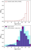 |
Fig. 18. Same as Fig. 17 but for the high-α sequence. Details are given in the text. |
| In the text | |
|
Fig. 19. Panels a and b: same as Fig. 5 for the parallel model results. The dashed black line depicts the low-α model phase, whereas the black solid line stands for the high-α phase. In the latter case, the thin line shows the period of the evolution when the number of stars born in age bins of 1 Gyr is smaller than 2% of total number of stars formed. Panels c and d: chemical evolution model results where we have taken into account estimated age and [M/H] errors. Analogously to the thin solid line in the upper two panels, smaller purple starred symbols are associated to stars with ages lower than 8 Gyr (before the inclusion of age errors). Details are given in the text. |
| In the text | |
|
Fig. 20. Abundance ratios of [α/Fe] as a function of [Fe/H] predicted by means of the parallel chemical evolution model including age and [M/H] errors for the high-α and low-α model phases (empty magenta and green pentagons, respectively). Both models and data are related to stars older than 11 Gyr. |
| In the text | |
Current usage metrics show cumulative count of Article Views (full-text article views including HTML views, PDF and ePub downloads, according to the available data) and Abstracts Views on Vision4Press platform.
Data correspond to usage on the plateform after 2015. The current usage metrics is available 48-96 hours after online publication and is updated daily on week days.
Initial download of the metrics may take a while.