| Issue |
A&A
Volume 622, February 2019
|
|
|---|---|---|
| Article Number | A198 | |
| Number of page(s) | 8 | |
| Section | Stellar structure and evolution | |
| DOI | https://doi.org/10.1051/0004-6361/201834635 | |
| Published online | 19 February 2019 | |
Properties of the transient X-ray pulsar Swift J1816.7–1613 and its optical companion
1
Department of Physics and Astronomy, University of Turku, 20014, Finland
e-mail: This email address is being protected from spambots. You need JavaScript enabled to view it.
2
Space Research Institute, Russian Academy of Sciences, Profsoyuznaya str. 84/32, Moscow 117997, Russia
3
Nordita, KTH Royal Institute of Technology and Stockholm University, Roslagstullsbacken 23, 10691 Stockholm, Sweden
4
Sobolev Astronomical Institute, Saint Petersburg State University, Staryj Peterhof, Saint Petersburg 198504, Russia
Received:
13
November
2018
Accepted:
8
January
2019
Abstract
We present results of investigation of the poorly studied X-ray pulsar Swift J1816.7–1613 during its transition from the type I outburst to the quiescent state. Our studies are based on the data obtained from X-ray observatories Swift, NuSTAR, and Chandra alongside with the latest IR data from UKIDSS/GPS and Spitzer/GLIMPSE surveys. The aim of the work is to determine the parameters of the system, namely the strength of the neutron star magnetic field and the distance to the source, which are required for the interpretation of the source behaviour in the framework of physically motivated models. No cyclotron absorption line was detected in the broad-band energy spectrum. However, the timing analysis hints at the typical for the X-ray pulsars magnetic field from a few ×1011 to a few ×1012 G. We also estimated the type of the IR-companion as a B0-2e star located at a distance of 7–13 kpc.
Key words: accretion, accretion disks / magnetic fields / pulsars: individual: Swift J1816.7–1613 / X-rays: binaries / stars: neutron
© ESO 2019
1. Introduction
The transient X-ray pulsar (XRP) Swift J1816.7–1613 was first detected by the Swift/BAT monitor on March 24, 2008 (Krimm et al. 2008). Pulsations with a period of 142.9 ± 0.2 s were discovered in the archival Chandra/ACIS data obtained serendipitously on February 11, 2007 (Halpern & Gotthelf 2008). An analysis of two other observations of the source performed by RXTE/PCA on March 29 and April 7, 2008, revealed a weighted average pulse period of 143.2 ± 0.1 s (Krimm et al. 2013), with a hint of the spin-up between these two observations with Ṗ = −5.93 × 10⁻⁷ s s−1.
Based on the observed periodicity of the outbursts detected by Swift/BAT, Corbet & Krimm (2014) proposed an orbital period of 151.4 ± 1.0 d for the system. However, La Parola et al. (2014) reported a different orbital period of 118.5 ± 0.8 d using a 113-month BAT survey. Recently, Corbet et al. (2017) searched for the periodicity of the system by performing power spectral analysis covering two different time intervals. First, they used the full BAT light curve of the source and found an orbital period of 151.1 ± 0.5 d, which is consistent with the period reported by Corbet & Krimm (2014), but they did not detect the orbital period of 118.5 d. Second, Corbet et al. (2017) considered the same time restrictions as La Parola et al. (2014) used in their analysis and found a period of 118.9 ± 0.6 d. Corbet et al. (2017) stated that the difference between the orbital periods is mainly because of the different time intervals used and that they both may be not actual orbital periods of the source.
The energy spectrum of Swift J1816.7–1613 obtained with the Chandra observatory on February 11, 2007, was described by a simple power-law model with a photon index of Γ = 1.2, modified by the photoelectric absorption with NH = 1.2 × 1023 cm−2, resulting in a flux of 4 × 10⁻¹² erg cm−2 s−1 in the 2–10 keV energy band (Halpern & Gotthelf 2008). The broad-band combined Swift/XRT and BAT spectrum obtained from the outburst episodes in the energy range of 0.2–150 keV was analysed by La Parola et al. (2014). It was modelled by a power-law model with a photon index of Γ ∼ 0.1 with a high energy cut-off at ∼10 keV, resulting in the average flux of about 1.3 × 10⁻¹⁰ erg cm−2 s−1 in the 0.2–150 keV energy range. The column density was estimated to be NH = 1.0 × 1023 cm−2, which is significantly higher than the average Galactic value in the source direction of 1.35 × 1022 cm−2 obtained from NHTOT (Willingale et al. 2013)1. The authors also derived the off-outburst flux from the source of ≈2.9 × 10⁻¹² erg cm−2 s−1 in the same energy band. Swift J1816.7–1613 was also detected by BeppoSAX in September 29, 1998, with a flux of 3.6 × 10⁻¹¹ erg cm−2 s−1 in 15–30 keV (Orlandini & Frontera 2008) and by XMM-Newton under the name 2XMM J181642.7–161320 on March 8, 2003, at the lowest flux of 7 × 10⁻¹³ erg cm−2 s−1 in the 0.2–12 keV band (Halpern & Gotthelf 2008).
The nature of the companion star in this system has not been determined yet. The archival Swift/UVOT observations of the source in the given Chandra location did not show any optical counterpart. However, taking into account the pulse and orbital periods and their location in the Corbet diagram for high-mass X-ray binaries (Corbet 1986), both Corbet & Krimm (2014) and La Parola et al. (2014) argued that the type of system is consistent with a Be/neutron star binary.
The magnetic field of the neutron star (NS) in Swift J1816.7–1613 has never been measured, and the properties of the system in the hard X-ray band remained unknown. In the current work we use our single NuSTAR observation in the hard X-rays, multiple archival observations in the standard X-ray energy band, and the infrared (IR) data in order to determine the properties of the system and its optical companion.
2. Observations and data reduction
This study is based on the data provided by three X-ray space satellites Swift, Chandra, and NuSTAR and the latest public IR data from the UKIDSS/GPS and Spitzer/GLIMPSE surveys. The details of the X-ray observations are given in Table 1. For all timing and spectral analysis we use HEASOFT 6.22.12 and XSPEC version 12.9.1p3.
X-ray observations of Swift J1816.7–1613.
2.1. Swift/XRT observations
Swift J1816.7–1613 was observed by the XRT telescope (Burrows et al. 2005) on board the Neil Gehrels Swift Observatory (Gehrels et al. 2004) multiple times in 2008 and 2017 with total exposures of 10.2 and 23 ks, respectively (see Table 1). All the Swift observations used in this study were obtained by the XRT telescope in the photon counting (PC) mode. To produce the cleaned event files (level 2) from level 1 products, the XRTPIPELINE tool from the XRTDAS package v3.4.04 was used. Also, we used XSELECT V2.4d with the standard criteria to reduce and analyse Swift/XRT data of Swift J1816.7–1613. We extracted the X-ray spectrum and the light curve of the source for every single observation in the energy range of 0.5–10 keV using circular region with a radius of 25″. The background spectra and light curves, likewise, were extracted from a source-free region with radius of 50″. The standard grade filtering (0–12 for PC) was used for the analysis. In order to calculate the ancillary response files for each observation, we used the task XRTMKARF.
2.2. Chandra observations
Swift J1816.7–1613 was also observed by the Chandra (Weisskopf et al. 1996) advanced CCD Imaging Spectrometer (ACIS; Garmire et al. 2003) for about 16 ks on February 11, 2007 (MJD 54142; ObsID 6689). The source was placed at the ACIS-S2 with no gratings in use yielding a moderate energy resolution. To reproduce and reprocess the archival level 1 data, the standard pipeline processing was performed using the software packages CIAO v4.9 (Fruscione et al. 2006) with a suitable CALDB v4.7.7. The source and background light curves and spectra were extracted from circular regions of the same radius of 20″.
2.3. NuSTAR observation
The Nuclear Spectroscopic Telescope Array (NuSTAR), launched on June 13, 2012, is the first focusing hard X-ray telescope operating in a wide energy range of 3–79 keV (Harrison et al. 2013). It consists of two co-aligned grazing incidence X-ray telescope systems which provide imaging resolution of 18″ (full width at half maximum, FWHM). The instruments have the spectral energy resolution of 400 eV (FWHM) at 10 keV.
In order to reduce the raw observational data, we performed the standard data reduction procedure described in the NuSTAR user guide5 using the NuSTAR Data Analysis Software NUSTARDAS v1.8.0 with a CALDB version 20180419. The source spectra and the light curves were extracted from a circular region with radius of 100″ for both FMPA and FMPB using NUPRODUCTS task (Fig. 1). The background photons were extracted from the source-free circular regions of the same radius located close to the source in the nearby chips because the background area in the source chip is contaminated by a faint X-ray source (bottom right corner of the source chip). Also, as shown in Fig. 1, a large fraction of the FPMA field of view is contaminated by stray light. The barycentric correction was applied to the resulting light curves using standard BARYCOR task and the position of the source from the XMM-Newton catalogue (source XMM J181642.7–161320).
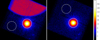 |
Fig. 1. NuSTAR image of Swift J1816.7–1613 extracted from FPMA (left panel) and FPMB (right panel) in the energy range of 3–79 keV. The solid white circles are the source extraction regions of radius 100″ and the dashed white circles are the background regions of the same radius which were selected from the source-free regions. The colour bar on the right hand side shows the number of counts per pixel. |
2.4. Infrared observations
In order to study the companion star in the IR band we use the latest data of the public release of UKIDSS/GPS6 and Spitzer/GLIMPSE7 surveys. Based on these surveys and the catalogue position of 2XMM J181642.7–161320 we can identify its IR counterpart as UGPS J181642.74–161322.2 or GLIMPSE:G014.5877+00.0913 (see Table 2).
Coordinates and IR-magnitudes of the counterpart of Swift J1816.7–1613 based on UKIDSS/GPS and Spitzer data.
3. Analysis and results
In this section we present the results of the timing and spectral analysis performed on X-ray data, and the analysis of the infrared observations.
3.1. Long-term light curve
To investigate the long-term variability of the source we use individual XRT observations obtained in 2017. The bolometric, absorption-corrected light curve is shown in the upper panel of Fig. 2.
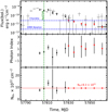 |
Fig. 2. Top panel: bolometric absorption-corrected X-ray light curve of Swift J1816.7–1613 obtained by Swift/XRT in 2017. Black points correspond to individual XRT observations and the red points show the observations in which we fixed the NH at the average value of 9.3 × 1022 cm−2. Grey points represent the 3-day-averaged Swift/BAT flux in the 15–50 keV band (in arbitrary units). Middle panel: variations in the power-law photon index. Bottom panel: variations in the hydrogen column density NH. The vertical green line indicates the date of our NuSTAR observation. |
First of all, we fitted individual spectra using a simple power law model modified with the photoelectric absorption (PHABS × PO in XSPEC). Due to low count rates all the spectra were binned to have at least one count in each energy channel and fitted using the W-statistics (Wachter et al. 1979). In order to find the bolometric flux from the source we converted the unabsorbed flux in the narrow energy band (0.5–10 keV) to a wider energy range (0.5–100 keV) using the bolometric correction factor Kbol = F0.5−100 keV/F0.5−10 keV. To calculate Kbol we used the simultaneous Swift/XRT and NuSTAR observations. From the measured fluxes F0.5−100 keV = 4.6 × 10⁻¹⁰ and F0.5−10 keV = 1.3 × 10⁻¹⁰ erg s−1 cm−2 (see Sect. 3.4), we estimated the bolometric correction factor Kbol ≈ 3.7. To find the X-ray flux in the 0.5–100 keV energy band, the spectral model (see Sect. 3.4) was extrapolated to 100 keV. We finally note that in our analysis the value of Kbol was assumed to be independent of the source flux.
The variability of the photon index and hydrogen column density calculated in the 0.5–10 keV band are shown in the middle and bottom panels of Fig. 2, respectively. For the three data points, shown with red dots, we fixed NH to the average value of 9.3 × 1022 cm−2 because of the low-count statistics. The last data point (around MJD 57860) presents the parameters obtained from the averaging of two nearby observations. The blue horizontal dashed lines show the source fluxes obtained from Chandra (MJD 54142) and XMM-Newton (MJD 52706) observations of 7.1 × 10⁻¹² and 7 × 10⁻¹³ erg s−1 cm−2 in the 2–10 keV energy band, respectively. For the two possible values of the orbital period of the system of 118.5 and 151.1 d, Chandra and XMM-Newton observations correspond to the different orbital phases not close to periastron. These fluxes, as well as the flux 2.9 × 10⁻¹² erg s−1 cm−2 obtained from XRT and BAT observations during the off-outburst state of the source (La Parola et al. 2014), suggest that the flux never drops much below ∼10−12 erg s−1 cm−2. The green dashed vertical line indicates the date of our NuSTAR observation.
As can be seen from Fig. 2 the peak of the outburst in both XRT and BAT data is reached around MJD 57800. It is worth mentioning that this date deviates by a few tens of days from the expectations derived using orbital period and phasing reported by La Parola et al. (2014) and Corbet et al. (2017). Most probably this is because both values of the orbital period of the source do not represent its true value due to the non-periodic behaviour of the source, as discussed in Corbet et al. (2017).
3.2. Pulse profile and pulsed fraction
Because no accurate orbital parameters required for the correction for the binary motion are available for the source, we used only the barycentric-corrected light curves in our temporal analysis. Therefore, the yielding periods might be affected by the orbital motion of the system. Using our NuSTAR data we obtained the spin period Pspin = 143.6863(2) s, which is consistent within errors with the value obtained by La Parola et al. (2014). The spin period and its uncertainty were obtained from the distribution of the results of the period search in 103 simulated light curves following procedure described by Boldin et al. (2013). To get the pulse period in each light curve, we use the standard EFSEARCH procedure from the FTOOLS package.
Thanks to the wide energy coverage of the NuSTAR observatory, we can study the pulse profile dependence on energy. We first extracted the barycentric-corrected light curves in five energy bands 3–7, 7–18, 18–30, 30–50, and 50–79 keV and then combined the individual light curves from modules FPMA and FPMB to get better statistics (see details in Krivonos et al. 2015).
Using the program EFOLD, the obtained light curves were folded with the pulse period to get the pulse profile in each energy band. The five top panels in Fig. 3 show the evolution of the pulse profile with increasing energy (from top to bottom). The pulse profiles have quite complicated structure with multiple peaks. The dominating features, the main maximum around phases 0.9–1.1 and the main minimum around phases 0.2–0.3 (zero phase was chosen arbitrarily), are shown by the dashed and dotted lines, respectively. The pulse profile demonstrates a clear dependence on energy. For instance, the right part of the main peak disappears at higher energies. To illustrate the energy dependence, we plotted the hardness ratio of the fluxes in the 7–18 and 3–7 keV bands in the bottom panel of Fig. 3. The described behaviour is clearly seen from the obvious decrease in the hardness ratio around the phase 0.1 (1.1). On the other hand there is a clear hardening of the emission at phases 0.7–0.9 (left wing of the main peak).
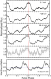 |
Fig. 3. Top panels: pulse profiles of Swift J1816.7–1613 in five different energy bands 3–7, 7–18, 18–30, 30–50, and 50–79 keV (from top to bottom) obtained with the NuSTAR observatory. The fluxes are normalized by the mean flux in each band. The position of the main maximum and minimum are shown by vertical dashed and dotted lines, respectively. The zero phase was chosen arbitrarily. Bottom panel: hardness ratio of Swift J1816.7–1613 pulse profiles in the energy bands 7–18 and 3–7 keV. The blue horizontal line indicates the hardness ratio of unity. |
The pulsed fraction calculated as PF = (Fmax − Fmin)/(Fmax + Fmin) is plotted as a function of energy in Fig. 4, where Fmin and Fmax are the minimum and maximum fluxes of the pulse profile, respectively. Below ∼30 keV the pulsed fraction has a nearly constant value around 45–50%. However, at energies above 30 keV, it increases above 60% that is typical for most XRPs (Lutovinov & Tsygankov 2009).
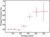 |
Fig. 4. Dependence of the pulsed fraction of Swift J1816.7–1613 on energy obtained from the NuSTAR observation. |
3.3. Power density spectrum
Figure 5 shows the power density spectrum (PDS) of the combined light curves from FPMA and FPMB in the full energy band. The PDS was calculated with the HEASOFT software task POWSPEC using a Miyamoto normalization. The Poisson noise level was estimated from the high-frequency 20–100 Hz part of the PDS and subtracted. The continuum of the PDS was fit with two models, a single power law and a broken power law. The regular pulsations at ≈143 s (0.007 Hz) and several harmonics are clearly visible in the PDS and were masked out for the fitting purposes. The simple power law with an index of −1.1 is able to fit the data very well. The broken power law deviates from the single power law only above ≈1 Hz and gives a poorly constrained break frequency of 2.4 ± 1.8 Hz, but does not significantly improve the quality of the fit. Therefore, we do not claim a detection of the break in the PDS. Rather, we take 0.6 Hz as a lower limit for the break frequency in order to estimate the NS magnetic field strength (see Sect. 4).
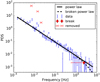 |
Fig. 5. Power density spectrum of Swift J1816.7–1613 obtained from combined light curves from FPMA and FPMB in the 3–79 keV energy band. The solid line represents a single power-law fit with index −1.1. Regular pulsations at ∼7 mHz and their harmonics were masked out in the fit. The dashed line is the broken power-law fit and the red diamond is the resulting break frequency at 2.4 ± 1.8 Hz. |
3.4. Spectral analysis
One of the main goals of this study was searching for the cyclotron resonant scattering feature (cyclotron absorption line) in the Swift J1816.7–1613 spectrum using the NuSTAR data. NuSTAR presents a unique sensitivity in the energy range where most of the known cyclotron absorption features have been detected so far (see Walter et al. 2015, for a review). First, we extracted the spectra using the described procedure from the NuSTAR and Swift observations performed simultaneously (Swift/XRT ObsID 00031188007). It allowed us to obtain and analyse in XSPEC a broad-band, 0.5–79 keV spectrum of Swift J1816.7–1613 for the first time.
The spectrum of the source has a shape typical of other accreting XRPs, demonstrating a cut-off at high energies (see e.g. Filippova et al. 2005). Although, the NuSTAR observation provided good statistics, we did not detect a cyclotron absorption line in the spectrum. To describe the spectral shape, we first fitted the spectrum using a cut-off power-law model modified by the photoelectric absorption PHABS × CUTOFFPL. This is the same model as was used by La Parola et al. (2014) to fit successfully the joint XRT and BAT spectrum of the source. However, for the better quality NuSTAR data it resulted in an unacceptable C-statistic value of 2006 (for 1576 d.o.f.). A better fit quality was obtained by using the Comptonization model of soft photons in a hot plasma (Titarchuk 1994), modified by the fluorescent iron line at 6.4 keV and photoelectric absorption PHABS (COMPTT + GAU). This composite model yielded a much lower C-value of 1477 (for 1572 d.o.f.).
The broad-band unfolded spectrum and the corresponding residuals from the best-fit model are shown in Fig. 6. In order to take into account the uncertainty in cross-calibration between different instruments we added the normalization factor to the model. It gives a normalization of 0.97 between NuSTAR instruments (FMPA and FMPB) and 0.63 between FMPA and Swift/XRT. The GAUSSIAN component representing an iron fluorescent emission line has peak at 6.44 keV and width of 0.21 keV. The best-fit parameters and their uncertainties are listed in Table. 3.
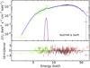 |
Fig. 6. Top panel: broad-band spectrum of Swift J1816.7–1613 obtained by NuSTAR/FPMA and FPMB (red and black crosses) and Swift/XRT (green crosses) together with the best-fit model CONSTANT × PHABS(COMPTT + GAUSSIAN) (solid line). Bottom panel: residuals from the best-fit model in units of standard deviations. |
Best-fit parameters for the joint NuSTAR and Swift/XRT spectrum approximation with CONSTANT × PHABS(COMPTT + GAUSSIAN) model.
We note that the best-fit value for the hydrogen column density NH = (6.3 ± 0.5)×1022 cm−2 is significantly higher than the Galactic mean value in this direction of 1.35 × 1022 cm−2 (Willingale et al. 2013). This difference can be due to either a significant intrinsic absorption in the system or some non-uniformities in the interstellar medium in the direction to the source that cannot be detected on the standard maps due to their angular resolution limits. The absorption value obtained in our analysis is somewhat lower than the value NH = (10.2 ± 0.5)×1022 cm−2 calculated by La Parola et al. (2014) in the direction to the source. This discrepancy can be caused by different spectral continuum models used in the mentioned work. For the same reason the NH obtained from the broad-band spectrum is lower than that derived from the individual Swift/XRT spectra (see the bottom panel of Fig. 2).
3.5. Identification of the IR companion
As was mentioned in Sect. 3.4, the absorption value measured from the X-ray spectrum exceeds significantly the Galactic value in the source direction. To determine the nature of Swift J1816.7–1613 we analysed IR properties of the counterpart according to the method proposed by Karasev et al. (2010, 2015a). The idea was to obtain photometric observations of an object in at least two filters, and to know the distance and the absorption up to the Galactic bulge in the direction of the studied object. After that we could evaluate the absorption magnitude to the source and roughly estimate the possible distance and the spectral class of the companion star.
To obtain reliable estimates of the absorption and other parameters using this method, we need to know a correct extinction law in the direction towards the source. Here we used a non-standard law AKs/E(J − Ks)≈0.43 and AKs/E(H − Ks)≈1.12 obtained for the Galactic bulge interstellar medium by Karasev et al. (2015a), Alonso-García et al. (2017), and Karasev & Lutovinov (2018). It is significantly different from the standard one (Cardelli et al. 1989) and more suitable for studying the central parts of the Galaxy.
In the next step, we were able to determine the magnitude of the absorption to the Galactic bulge using the position of the red clump giants (RCG) on the colour–magnitude diagram (CMD), reconstructed for all stars in a ∼3′ × 3′ vicinity around the object (Fig. 7, left panel). We note that all RCG stars have approximately the same luminosity and colour (they are weakly affected by the metallicity and the age). They form a compact and well-recognized clump on the red giant branch with the observed magnitude and colour of their centroid, KsRCG = 13.51 ± 0.05 and (J − Ks)RCG = 3.16 ± 0.04. Taking into account an absolute magnitude of RCG MKs, RCG ≈ −1.61 and their intrinsic colour (J − Ks)0 ≈ 0.68 (Alves 2000; Karasev et al. 2010; Gonzalez et al. 2012; Gontcharov 2017) we were able to estimate the extinction and the distance to these objects (and consequently to the bulge) as AKs = 1.06 ± 0.03 and D = 6.5 ± 0.2 kpc (here we used the relations AJ − AKs = (J − Ks)RGC − (J − Ks)0, AJ ≈ 3.33 × AKs in accordance with the above extinction law, as well as the relation 5 − 5logD = MKs, RCG − KsRCG + AKs, where D is the distance in pc)8. We note that the obtained distance to the bulge at l ≈ 14° agrees roughly with the extrapolation of the results of Gerhard & Martinez-Valpuesta (2012) to these Galactic longitudes.
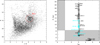 |
Fig. 7. Left panel: colour–magnitude diagram for all stars from UKIDSS/GPS sky survey (see Sect. 2.4) in the 3′ × 3′ vicinity around Swift J1816.7–1613. Red clump giants are marked by the red circle. Right panel: distance-absorption diagram that demonstrates which types of stars can be appropriate as counterparts for Swift J1816.7–1613 (white areas). The stars (cyan crosses for Be stars and black crosses for other stars) located in the grey areas of the diagram cannot be counterparts (see text for details). The black dashed lines represent the absorption and distance to the Galactic bulge. |
Once we determined the distance and absorption to the Galactic bulge in the source direction, we could proceed to estimate the absorption to the source as well as its class and the distance. Assuming stars of different spectral and luminosity classes as a counterpart of Swift J1816.7–1613 we could define a correction for the absorption and distance required for each of them to satisfy the observed magnitudes9. As a result we obtained the distance-absorption diagram (Fig. 7, right panel), where classes of stars that potentially could be a companion of Swift J1816.7–1613 are located in white areas, i.e. if the star is located in front of the bulge, the absorption to it should be lower than the absorption to the bulge, and vice versa. Stars that cannot be a companion are located in grey areas. Dashed lines correspond to the absorption and distance to the Galactic bulge and divide the diagram into the above mentioned areas. We note that we do not know precisely where the extinction law becomes non-standard; therefore, for stars located in front of the bulge we used a standard extinction law, and for stars in the bulge or behind it the non-standard law was applied (for a detailed description of the method, see Karasev et al. 2015a).
From the distance-absorption diagram we could make the first essential conclusion: the absorption magnitude to Swift J1816.7–1613 is AKs ≈ 3.0. Additionally, the source counterpart belongs to the stars with classes not later than B2-3 for main sequence or Be-stars, which are located at distances greater than ≈7 kpc (Fig. 7, right panel). At the same time from the source behaviour in the X-rays and the Corbet diagram, we have indirect indications that the companion of Swift J1816.7–1613 is probably a Be-star (Corbet & Krimm 2014; La Parola et al. 2014). From Fig. 7 we can see that stars of B0-2e or early classes located at the distances of 7–13 kpc can be appropriate companions. We note that we are not able to relate the absorption measured in the X-rays towards the source (NH) to the magnitude of AKs using standard relations (see e.g. Güver & Özel 2009) because the extinction law towards the source is not the standard one (see above). Thus, we are unable to compare the IR and X-ray results directly and dedicated spectroscopic observations in the near IR band are required to firmly establish the nature of the companion star in Swift J1816.7–1613.
4. Discussion
In this work, we presented a detailed investigation of the transient XRP Swift J1816.7–1613 both in X-ray and infrared bands. One of our main goals was to estimate the fundamental physical parameters of the source such as the magnetic field of the NS. The most straightforward way to determine the magnetic field in such systems is to find the cyclotron absorption line in its spectrum. No such feature was detected through the spectral analysis of the NuSTAR data. The lack of the cyclotron absorption line suggests that the magnetic field in Swift J1816.7–1613 is either weaker than ∼5 × 10¹¹ G or stronger than ∼6 × 10¹² G considering the lower and upper limits of the NuSTAR energy range where sensitivity allows us to exclude presence of such feature.
In the literature one can find other indirect methods to estimate the strength of the magnetic field in XRPs. However, all such models require a knowledge of the mass accretion rate onto the NS, and hence the distance to the system. For the following discussion we use the distance D = 10 kpc obtained in Sect. 3.5.
One of indirect methods to estimate the magnetic field is to use the so-called propeller effect (Illarionov & Sunyaev 1975; Stella et al. 1986). In the propeller regime, the accretion would be prohibited by the centrifugal barrier caused by the rotating magnetosphere of the NS if the magnetospheric radius is larger than the corotation radius (Rm > Rc). It happens at the critical luminosity Lprop, which is a function of the pulse period and magnetic field strength (see e.g. Campana et al. 2002). As a result of the propeller effect, the source luminosity drops sharply by about two orders of magnitude for a typical XRP. The method of the magnetic field estimate based on the measurement of the critical luminosity Lprop was recently calibrated using XRPs with known magnetic fields (Tsygankov et al. 2016; Lutovinov et al. 2017). In order to detect the propeller effect, we organized a Swift/XRT monitoring of Swift J1816.7–1613 however, no sharp drop in the flux was found in the tail of the studied outburst (Fig. 2).
Instead of the transition to the propeller regime, the source light curve shows a slowdown of the flux decline at the level of a few ×10−12 erg s−1 cm−2 (see top panel of Fig. 2), which corresponds to the source luminosity of a few ×1034 erg s−1. Although, the XRT monitoring was not long enough to cover a full orbital cycle, the source fluxes measured by Chandra and XMM-Newton (2.6 × 10⁻¹¹ and 2.6 × 10⁻¹² erg s−1 cm−2 after bolometric correction, respectively) as well as the off-outburst flux of 2.9 × 10⁻¹² erg s−1 cm−2 obtained by XRT and BAT (La Parola et al. 2014) confirm that the system does not transit to the propeller regime at any orbital phase between type I outbursts. This behaviour is very similar to what was recently revealed in another transient XRP, GRO J1008-57, where the luminosity stopped its fading around 1035 erg s−1 (Tsygankov et al. 2017). This was interpreted as a transition of the source to the stable accretion from the “cold” low-ionization disc (Lasota 2001). Based on the analogy with GRO J1008-57, where the magnetic field is known from the cyclotron line, and using Eq. (6) from Tsygankov et al. (2017) one can expect the magnetic field in Swift J1816.7–1613 to be below ∼1013 G.
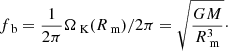
Another indirect method for evaluating the magnetic field of the NS is based on the possibility of estimating the inner radius of the accretion disc (or magnetospheric radius) from the properties of the PDS. The origin of the flux variability can be explained with the perturbation propagation model (Lyubarskii 1997). In the framework of this model, stochastic viscous processes in the accretion disc perturb the mass accretion rate at a given radius on timescales close to the local Keplerian frequency. The resulting PDS of the mass accretion rate at the inner disc radius can be described with the power law up to the maximum frequency that can be generated in the disc (Lyubarskii 1997; Mushtukov et al. 2018). In the case of XRPs, due to the strong magnetic field of the NS, the disc is truncated by the magnetosphere at the radius
 (1)
(1)
where ξ is a parameter describing the accretion geometry, typically taken to be 0.5; M is the NS mass in units of solar masses; R6 is the NS radius in units of 106 cm; B12 is the magnetic field strength in units of 1012 G; and L37 is the luminosity in units of 1037 erg s−1 (Lamb et al. 1973).
At smaller radii the noise is not generated and one can expect a break, i.e. a steepening of the power-law index from ∼−1 to ∼−2, in the PDS at maximum frequency fb corresponding to the magnetospheric radius. As a first approximation, the break frequency is related to the Keplerian orbital frequency ΩK at the innermost radius of the disc and offers a way to connect the power spectrum feature to the magnetic field (Revnivtsev et al. 2009; Tsygankov et al. 2012; Doroshenko et al. 2014):
 (2)
(2)
The PDS based on the NuSTAR data presented in Fig. 5 does not exhibit a significant break and can be fit well with a simple power law. Based on the broken power-law fit, we can give only a lower limit estimate to the break frequency, fb ≳ 0.6 Hz. From Eq. (2) we see that in this case the inner radius has to be smaller than 2.4 × 108 cm. Assuming luminosity during our NuSTAR observation of 5.5 × 1036 erg s−1 and using Eq. (1), we can estimate an upper limit for the magnetic field B ≲ 2 × 10¹² G, which is within the standard range of magnetic fields for XRPs. If, however, the initial mass accretion rate fluctuations are driven by the dynamo process at frequency a few times below the local Keplerian one (King et al. 2004), the resulting magnetic field strength might be even lower by about the same factor.
5. Conclusions
In this work, we presented the results of the X-ray and IR analysis of the poorly studied XRP Swift J1816.7–1613 and its optical companion during the transition from type I outburst to the quiescent state. Data obtained from the Chandra, Swift, and NuSTAR observatories along with data from the UKIDSS/GPS and Spitzer/GLIMPSE surveys were used. The aim of this study was to describe properties of the source in the hard X-ray band as well as its optical companion for the first time. To estimate the distance to the source and the nature of the companion star, we performed an analysis of IR data. As a result, it is suggested that the companion star in this system can be classified as a B0-2e star located at a distance of 7–13 kpc. We attempted to estimate the strength of the NS magnetic field using different methods. The spectral analysis revealed no cyclotron line in the NuSTAR broad-band spectrum, which corresponds to the magnetic field B ≲ 5 × 10¹¹ or B ≳ 6 × 10¹² G. According to the long-term light curve, the system does not switch to the propeller state, keeping a relatively high luminosity of about 1034–1035 erg s−1 between type I outbursts. Using the similarity of this behaviour to that of another transient Be/XRP GRO J1008-57, and based on the cold disc model, the magnetic field can be roughly estimated as B ≲ 1013 G. Another method based on the properties of the fast flux variability resulted in a lower value of an upper limit for the magnetic field strength B ≲ 2 × 10¹² G. It is important to note that these methods are applicable only in the case of accretion from the disc. More sensitive observations in the low state are required to make final conclusions.
The absolute magnitude of RGC was previously converted to the UKIRT system using transformation formulas from http://www.astro.caltech.edu/~jmc/2mass/v3/transformations/
Absolute magnitudes and intrinsic colours of stars of different spectral and luminosity classes for the corresponding filters were taken from Wegner (2000, 2006, 2007, 2014) and Wegner (2015) for Be-stars.
Acknowledgments
This study was supported by the grant TM-17-10606 of the Finnish National Agency for Education (AN); the Academy of Finland travel grants 309228, 316932, and 317552 (SST, JP); and the Russian Foundation for Basic Research projects 16-02-00294 (DIK) and 17-52-80139 BRICS-a (AAL, SST). This work is based in part on data of the UKIRT Infrared Deep Sky Survey. In addition, part of this work is based on observations made with the Spitzer Space Telescope, which is operated by the Jet Propulsion Laboratory, California Institute of Technology under a contract with NASA. We express our thanks to the NuSTAR and Swift teams for the prompt scheduling and execution of our observations. We also acknowledge the support from the COST Actions CA16214 and CA16104.
References
- Alonso-García, J., Minniti, D., Catelan, M., et al. 2017, ApJ, 849, L13 [NASA ADS] [CrossRef] [Google Scholar]
- Alves, D. R. 2000, ApJ, 539, 732 [NASA ADS] [CrossRef] [MathSciNet] [Google Scholar]
- Boldin, P. A., Tsygankov, S. S., & Lutovinov, A. A. 2013, Astron. Lett., 39, 375 [NASA ADS] [CrossRef] [Google Scholar]
- Burrows, D. N., Hill, J. E., Nousek, J. A., et al. 2005, Space Sci. Rev., 120, 165 [NASA ADS] [CrossRef] [Google Scholar]
- Campana, S., Stella, L., Israel, G. L., et al. 2002, ApJ, 580, 389 [NASA ADS] [CrossRef] [Google Scholar]
- Cardelli, J. A., Clayton, G. C., & Mathis, J. S. 1989, ApJ, 345, 245 [NASA ADS] [CrossRef] [Google Scholar]
- Corbet, R. H. D. 1986, MNRAS, 220, 1047 [NASA ADS] [CrossRef] [Google Scholar]
- Corbet, R. H. D., & Krimm, H. A. 2014, ATel, 6253 [Google Scholar]
- Corbet, R. H. D., Coley, J. B., & Krimm, H. A. 2017, ApJ, 846, 161 [NASA ADS] [CrossRef] [Google Scholar]
- Doroshenko, V., Santangelo, A., Doroshenko, R., et al. 2014, A&A, 561, A96 [NASA ADS] [CrossRef] [EDP Sciences] [Google Scholar]
- Filippova, E. V., Tsygankov, S. S., Lutovinov, A. A., & Sunyaev, R. A. 2005, Astron. Lett., 31, 729 [NASA ADS] [CrossRef] [Google Scholar]
- Fruscione, A., McDowell, J. C., Allen, G. E., et al. 2006, in Observatory Operations: Strategies, Processes, and Systems, eds. D. R. Silva, & R. E. Doxsey, Proc. SPIE, 6270, 62701V [CrossRef] [Google Scholar]
- Garmire, G. P., Bautz, M. W., Ford, P. G., Nousek, J. A., & Ricker, Jr., G. R. 2003, in X-Ray and Gamma-Ray Telescopes and Instruments for Astronomy, eds. J. E. Truemper, & H. D. Tananbaum, Proc. SPIE, 4851, 28 [Google Scholar]
- Gehrels, N., Chincarini, G., Giommi, P., et al. 2004, ApJ, 611, 1005 [NASA ADS] [CrossRef] [Google Scholar]
- Gerhard, O., & Martinez-Valpuesta, I. 2012, ApJ, 744, L8 [NASA ADS] [CrossRef] [Google Scholar]
- Gontcharov, G. A. 2017, Astron. Lett., 43, 545 [NASA ADS] [CrossRef] [Google Scholar]
- Gonzalez, O. A., Rejkuba, M., Zoccali, M., et al. 2012, A&A, 543, A13 [NASA ADS] [CrossRef] [EDP Sciences] [Google Scholar]
- Güver, T., & Özel, F. 2009, MNRAS, 400, 2050 [NASA ADS] [CrossRef] [Google Scholar]
- Halpern, J. P., & Gotthelf, E. V. 2008, ATel, 1457 [Google Scholar]
- Harrison, F. A., Craig, W. W., Christensen, F. E., et al. 2013, ApJ, 770, 103 [NASA ADS] [CrossRef] [Google Scholar]
- Illarionov, A. F., & Sunyaev, R. A. 1975, A&A, 39, 185 [NASA ADS] [Google Scholar]
- Karasev, D. I., & Lutovinov, A. A. 2018, Astron. Lett., 44, 220 [NASA ADS] [CrossRef] [Google Scholar]
- Karasev, D. I., Lutovinov, A. A., & Burenin, R. A. 2010, MNRAS, 409, L69 [NASA ADS] [CrossRef] [Google Scholar]
- Karasev, D. I., Tsygankov, S. S., & Lutovinov, A. A. 2015a, Astron. Lett., 41, 394 [NASA ADS] [CrossRef] [Google Scholar]
- King, A. R., Pringle, J. E., West, R. G., & Livio, M. 2004, MNRAS, 348, 111 [NASA ADS] [CrossRef] [Google Scholar]
- Krimm, H. A., Barthelmy, S. D., Baumgartner, W., et al. 2008, ATel, 1456 [Google Scholar]
- Krimm, H. A., Holland, S. T., Corbet, R. H. D., et al. 2013, ApJS, 209, 14 [NASA ADS] [CrossRef] [Google Scholar]
- Krivonos, R. A., Tsygankov, S. S., Lutovinov, A. A., et al. 2015, ApJ, 809, 140 [NASA ADS] [CrossRef] [Google Scholar]
- La Parola, V., Segreto, A., Cusumano, G., et al. 2014, MNRAS, 445, L119 [NASA ADS] [CrossRef] [Google Scholar]
- Lamb, F. K., Pethick, C. J., & Pines, D. 1973, ApJ, 184, 271 [NASA ADS] [CrossRef] [Google Scholar]
- Lasota, J.-P. 2001, New Astron. Rev., 45, 449 [NASA ADS] [CrossRef] [Google Scholar]
- Lutovinov, A. A., & Tsygankov, S. S. 2009, Astron. Lett., 35, 433 [NASA ADS] [CrossRef] [Google Scholar]
- Lutovinov, A. A., Tsygankov, S. S., Krivonos, R. A., Molkov, S. V., & Poutanen, J. 2017, ApJ, 834, 209 [NASA ADS] [CrossRef] [Google Scholar]
- Lyubarskii, Y. E. 1997, MNRAS, 292, 679 [NASA ADS] [CrossRef] [Google Scholar]
- Mushtukov, A. A., Ingram, A., & van der Klis, M. 2018, MNRAS, 474, 2259 [NASA ADS] [CrossRef] [Google Scholar]
- Orlandini, M., & Frontera, F. 2008, ATel, 1462 [Google Scholar]
- Revnivtsev, M., Churazov, E., Postnov, K., & Tsygankov, S. 2009, A&A, 507, 1211 [NASA ADS] [CrossRef] [EDP Sciences] [Google Scholar]
- Stella, L., White, N. E., & Rosner, R. 1986, ApJ, 308, 669 [NASA ADS] [CrossRef] [Google Scholar]
- Titarchuk, L. 1994, ApJ, 434, 570 [NASA ADS] [CrossRef] [Google Scholar]
- Tsygankov, S. S., Krivonos, R. A., & Lutovinov, A. A. 2012, MNRAS, 421, 2407 [NASA ADS] [CrossRef] [Google Scholar]
- Tsygankov, S. S., Lutovinov, A. A., Doroshenko, V., et al. 2016, A&A, 593, A16 [NASA ADS] [CrossRef] [EDP Sciences] [Google Scholar]
- Tsygankov, S. S., Mushtukov, A. A., Suleimanov, V. F., et al. 2017, A&A, 608, A17 [NASA ADS] [CrossRef] [EDP Sciences] [Google Scholar]
- Wachter, K., Leach, R., & Kellogg, E. 1979, ApJ, 230, 274 [Google Scholar]
- Walter, R., Lutovinov, A. A., Bozzo, E., & Tsygankov, S. S. 2015, A&ARv, 23, 2 [NASA ADS] [CrossRef] [Google Scholar]
- Wegner, W. 2000, MNRAS, 319, 771 [NASA ADS] [CrossRef] [Google Scholar]
- Wegner, W. 2006, MNRAS, 371, 185 [NASA ADS] [CrossRef] [Google Scholar]
- Wegner, W. 2007, MNRAS, 374, 1549 [NASA ADS] [CrossRef] [Google Scholar]
- Wegner, W. 2014, Acta Astron., 64, 261 [NASA ADS] [Google Scholar]
- Wegner, W. 2015, Astron. Nachr., 336, 159 [NASA ADS] [CrossRef] [Google Scholar]
- Weisskopf, M. C., O’Dell, S. L., & van Speybroeck, L. P. 1996, in Multilayer and Grazing Incidence X-Ray/EUV Optics III, eds. R. B. Hoover, & A. B. Walker, Proc. SPIE, 2805, 2 [NASA ADS] [CrossRef] [Google Scholar]
- Willingale, R., Starling, R. L. C., Beardmore, A. P., Tanvir, N. R., & O’Brien, P. T. 2013, MNRAS, 431, 394 [NASA ADS] [CrossRef] [Google Scholar]
All Tables
Coordinates and IR-magnitudes of the counterpart of Swift J1816.7–1613 based on UKIDSS/GPS and Spitzer data.
Best-fit parameters for the joint NuSTAR and Swift/XRT spectrum approximation with CONSTANT × PHABS(COMPTT + GAUSSIAN) model.
All Figures
|
Fig. 1. NuSTAR image of Swift J1816.7–1613 extracted from FPMA (left panel) and FPMB (right panel) in the energy range of 3–79 keV. The solid white circles are the source extraction regions of radius 100″ and the dashed white circles are the background regions of the same radius which were selected from the source-free regions. The colour bar on the right hand side shows the number of counts per pixel. |
| In the text | |
|
Fig. 2. Top panel: bolometric absorption-corrected X-ray light curve of Swift J1816.7–1613 obtained by Swift/XRT in 2017. Black points correspond to individual XRT observations and the red points show the observations in which we fixed the NH at the average value of 9.3 × 1022 cm−2. Grey points represent the 3-day-averaged Swift/BAT flux in the 15–50 keV band (in arbitrary units). Middle panel: variations in the power-law photon index. Bottom panel: variations in the hydrogen column density NH. The vertical green line indicates the date of our NuSTAR observation. |
| In the text | |
|
Fig. 3. Top panels: pulse profiles of Swift J1816.7–1613 in five different energy bands 3–7, 7–18, 18–30, 30–50, and 50–79 keV (from top to bottom) obtained with the NuSTAR observatory. The fluxes are normalized by the mean flux in each band. The position of the main maximum and minimum are shown by vertical dashed and dotted lines, respectively. The zero phase was chosen arbitrarily. Bottom panel: hardness ratio of Swift J1816.7–1613 pulse profiles in the energy bands 7–18 and 3–7 keV. The blue horizontal line indicates the hardness ratio of unity. |
| In the text | |
|
Fig. 4. Dependence of the pulsed fraction of Swift J1816.7–1613 on energy obtained from the NuSTAR observation. |
| In the text | |
|
Fig. 5. Power density spectrum of Swift J1816.7–1613 obtained from combined light curves from FPMA and FPMB in the 3–79 keV energy band. The solid line represents a single power-law fit with index −1.1. Regular pulsations at ∼7 mHz and their harmonics were masked out in the fit. The dashed line is the broken power-law fit and the red diamond is the resulting break frequency at 2.4 ± 1.8 Hz. |
| In the text | |
|
Fig. 6. Top panel: broad-band spectrum of Swift J1816.7–1613 obtained by NuSTAR/FPMA and FPMB (red and black crosses) and Swift/XRT (green crosses) together with the best-fit model CONSTANT × PHABS(COMPTT + GAUSSIAN) (solid line). Bottom panel: residuals from the best-fit model in units of standard deviations. |
| In the text | |
|
Fig. 7. Left panel: colour–magnitude diagram for all stars from UKIDSS/GPS sky survey (see Sect. 2.4) in the 3′ × 3′ vicinity around Swift J1816.7–1613. Red clump giants are marked by the red circle. Right panel: distance-absorption diagram that demonstrates which types of stars can be appropriate as counterparts for Swift J1816.7–1613 (white areas). The stars (cyan crosses for Be stars and black crosses for other stars) located in the grey areas of the diagram cannot be counterparts (see text for details). The black dashed lines represent the absorption and distance to the Galactic bulge. |
| In the text | |
Current usage metrics show cumulative count of Article Views (full-text article views including HTML views, PDF and ePub downloads, according to the available data) and Abstracts Views on Vision4Press platform.
Data correspond to usage on the plateform after 2015. The current usage metrics is available 48-96 hours after online publication and is updated daily on week days.
Initial download of the metrics may take a while.