| Issue |
A&A
Volume 622, February 2019
|
|
|---|---|---|
| Article Number | A62 | |
| Number of page(s) | 12 | |
| Section | Cosmology (including clusters of galaxies) | |
| DOI | https://doi.org/10.1051/0004-6361/201834383 | |
| Published online | 30 January 2019 | |
Screenings in modified gravity: a perturbative approach
1
Consejo Nacional de Ciencia y Tecnología, Av. Insurgentes Sur 1582, Colonia Crédito Constructor, Del. Benito Jurez 03940, Ciudad de México, Mexico
2
Departamento de Física, Instituto Nacional de Investigaciones Nucleares, Apartado Postal 18-1027, Col. Escandon, Ciudad de México 11801, Mexico
3
Institute Of Theoretical Astrophysics, University of Oslo, 0315 Oslo, Norway
e-mail: This email address is being protected from spambots. You need JavaScript enabled to view it.
Received:
5
October
2018
Accepted:
29
November
2018
Abstract
We present a formalism to study screening mechanisms in modified theories of gravity through perturbative methods in different cosmological scenarios. We consider Einstein-frame posed theories that are recast as Jordan-frame theories, where a known formalism is employed, although the resulting nonlinearities of the Klein–Gordon equation acquire an explicit coupling between matter and the scalar field, which is absent in Jordan-frame theories. The obtained growth functions are then separated into screening and non-screened contributions to facilitate their analysis. This allows us to compare several theoretical models and to recognize patterns that can be used to distinguish models and their screening mechanisms. In particular, we find anti-screening features in the symmetron model. In contrast, chameleon-type theories in both the Jordan and Einstein frames always present a screening behaviour. Up to third order in perturbation, we find no anti-screening behaviour in theories with a Vainshtein mechanism, such as the Dvali Gabadadze Porrati braneworld model and the cubic Galileon.
Key words: gravitation / large-scale structure of Universe / cosmology: theory / cosmology: miscellaneous / cosmology: observations / dark energy
© ESO 2019
1. Introduction
Two decades have passed since the discovery of the present-day acceleration of the Universe (Riess et al. 1998; Perlmutter et al. 1999). Its physical origin, however, is still a mystery. The simplest choice is that this acceleration is the result of the vacuum energy, in the form of a cosmological constant, in Einstein’s equations. This model is in agreement with current observations, but is plagued by the fine-tuning problem. Another simple option is that dark energy is a dynamical field, as in quintessence models. This field may also interact with the dark matter sector, giving rise to interacting dark energy models (Amendola & Tsujikawa 2010).
Instead of modifying the particle content of the Universe, an alternative solution is extending Einstein gravity in such a way that the current acceleration of the Universe is accounted for. However, precise measurements on Earth, in the solar system, in binary pulsars, and of gravitational waves (LIGO Collaboration & Virgo Collaboration 2016; Bertotti et al. 2003; Will 2006; Williams et al. 2004) strongly constrain deviations); strongly constrain deviations from general relativity (GR) at these scales (Will 2014). This is a challenge to theories of gravity beyond Einstein GR, which claim to be an explanation of the present-day acceleration (Clifton et al. 2012; Joyce et al. 2015; Bull et al. 2016).
We note, however, that all these tests probe extensions to GR in astrophysical systems that reside in dense galactic environments. Conditions are therefore far from the cosmological background density, curvature, and even the gravitational potential differs from that of the background by several orders of magnitude (Baker et al. 2015).
A way of evading the high-density environmental constraints while still allowing deviations from GR on cosmological scales is to hide modifications to Einstein’s gravity in these environments. The idea is that the geometry is modified by introducing a new degree of freedom that drives the acceleration of the Universe. This degree of freedom, in the simplest case a scalar field, would be suppressed in high-density or curvature environments, however.
Several screening mechanisms have been proposed in the literature, and they can be classified in several ways (Joyce et al. 2015; Brax 2013; Brax & Davis 2015; Koyama 2016). We here investigate screening mechanisms that result from one of the following three properties: i) Weak coupling, in which the coupling to matter fields becomes weak in regions of high density, hence suppressing the fifth force. At large scales, where the density is low, the coupling becomes large and the fifth force acts strongly. Examples of theories of this type are symmetron models (Hinterbichler & Khoury 2010; Pietroni 2005; Olive & Pospelov 2008) and varying dilaton (Damour & Polyakov 1994; Brax et al. 2011). ii) Large mass, when the mass of the field becomes large in regions of high density, suppressing the range of the fifth force. At low densities, the scalar field mass is small and mediates a long range fifth force. Examples of this type are chameleons (Khoury & Weltman 2004a,b). Finally, iii) large inertia, when the scalar field kinetic function depends on the environment, being large in high dense regions (and then the Yukawa potential is suppressed) and small in low dense regions. Examples of the former are K-mouflage models (Babichev et al. 2009, 2011), and examples of the latter are Vainshtein models (Vainshtein 1972).
Screening mechanisms are a relatively generic prediction of viable modified gravity (MG) theories (Brax et al. 2012). Detecting them would therefore be a signature of physics beyond GR. Observational tests of screening focus on the transition between the fully screened and unscreened regimes, where deviations from GR are expected to be most pronounced. For viable cosmological models, this transition occurs in regions where the matter density and gravitational potential are nonlinear and start to approach their linear or background values: this can be observed in the outskirts of dark matter halos and their properties (e.g. Shirata et al. 2005; Davis et al. 2012; Oyaizu et al. 2008; Schmidt et al. 2009; Barreira et al. 2013; Wyman et al. 2013; Zhao 2014; Clifton et al. 2005; Lombriser et al. 2015, 2012; Martino & Sheth 2009; Clampitt et al. 2013; Llinares & Mota 2013; Hellwing et al. 2013; Gronke et al. 2014, 2015; Stark et al. 2016).
Screening mechanisms are in fact a nonlinear effect. Therefore, predictions of their signatures in astrophysical systems are computed by integrating the fully nonlinear equations of motion for the extra-degree of freedom of gravity and also using N-body simulations in order to simulate nonlinear structure formation. These computations are extremely time-consuming, however. It is therefore not viable to use them for a parameter estimation or even to place constraints on the parameter space of such theories using nonlinear codes of structure formation. It is then imperative to find other methods to describe and probe screening mechanisms in faster and accurate ways. Although screenings are more commonly studied in the highly nonlinear regime, they leave imprints on quasi-linear scales that can be captured by cosmological perturbation theory (PT) and should be considered in the low-density regions of large-scale structure formation; see for example (Koyama et al. 2009).
On the other hand, PT has experienced many developments in recent years (Matsubara 2008a; Baumann et al. 2012; Carlson et al. 2013), in part because it can be useful to analytically understand different effects in the power spectrum and correlation function for the dark matter clustering. These effects can be confirmed or refuted, and further explored with simulations to ultimately understand the outcomes of present and future galaxy surveys, such as eBOSS (Zhao 2016), DESI (Aghamousa et al. 2016), EUCLID (Amendola et al. 2013), and LSST (LSST Dark Energy Science Collaboration 2012). Two approaches have been used to study PT: the Eulerian standard PT (SPT) and Lagrangian PT (LPT), which both have advantages and drawbacks, but they are complementary in the end (Tassev 2014). The nonlinear PT for MG was developed initially in (Koyama et al. 2009), and has been further studied in several other works (Taruya et al. 2014a,b; Brax & Valageas 2013; Bellini & Zumalacarregui 2015; Taruya 2016; Bose & Koyama 2016, 2017; Barrow & Mota 2003; Akrami et al. 2013; Fasiello & Vlah 2017; Aviles & Cervantes-Cota 2017; Hirano et al. 2018; Bose et al. 2018; Bose & Taruya 2018; Aviles et al. 2018). The LPT for dark matter fluctuations in MG was developed in Aviles & Cervantes-Cota (2017), and further studies for biased tracers in Aviles et al. (2018). The PT for MG has the advantage that it allows us to understand the role that these physical parameters play in the screening features of dark matter statistics. We here study some of these effects through screening mechanisms by examining them at second- and third-order perturbation levels using PT for some MG models. To this end, we build on the LPT formalism developed in Aviles & Cervantes-Cota (2017), which was initially posited for MG theories in the Jordan frame, in order to apply it to theories in the Einstein frame. Because of the direct coupling of the scalar field and the dark matter in the Klein–Gordon equation, the equations that govern the screening can differ substantially from those in Jordan-frame MG theories. In general, screening effects depend on the type of nonlinearities that are introduced in the Lagrangian density. We present a detailed analysis of screening features and identify the theoretical roots of their origin. Our results show that screenings possess peculiar features that depend on the scalar field effective mass and couplings, and that may in particular cases cause anti-screening effects in the power spectrum, such as in the symmetron model. We perform this analysis by separating the growth functions into screening and non-screened parts. We note, however, that we do not compare the perturbative approach with a fully nonlinear simulation. We refer to (Koyama et al. 2009), for instance, for investigations like this at the level of the power spectrum.
This work is organized as follows: in Sect. 2 we set up the formalism for perturbation theory in both the Einstein and Jordan frames; in Sect. 3 we apply these methods to the specific gravity models investigated here; in Sect. 4 we show the matter power spectra and in Sect. 5 the screening growth function analysis. We conclude in Sect. 6 with a discussion of our results. Some formulae are displayed in Appendix A.
2. Perturbation theory in the Einstein frame
In this section we are interested in MG theories defined in the Einstein frame with action
![Mathematical equation: $$ \begin{aligned} S = \int \mathrm{d}^4x \sqrt{-{ g}} \left( \frac{M_{\mathrm{Pl} }^2}{2} R - (\nabla \varphi )^2 - V(\varphi ) \right) + S_{\rm m}[\tilde{ g}_{\mu \nu }], \end{aligned} $$](/articles/aa/full_html/2019/02/aa34383-18/aa34383-18-eq1.gif) (1)
(1)
with the conformal metric
 (2)
(2)
where C(φ) is a conformal factor (in the literature it is more common to find A(φ); we use C instead because A is used below to characterize the strength of the gravitational force). By taking variations of action Eq. (1) with respect to the scalar field, we obtain the Klein–Gordon equation
 (3)
(3)
where T is the trace of the energy momentum tensor of matter. In PT we split the scalar field into background  and perturbed δφ parts,
 (4)
(4)
Hereafter, a bar over a dynamical quantity means that we refer to its homogeneous and isotropic background value; we also assume a dark matter perfect fluid with T = − ρ. In the following we adopt the quasi-static limit for the perturbed piece, which relies on neglecting temporal derivatives in the Klein–Gordon equation, thus Eq. (3) becomes
![Mathematical equation: $$ \begin{aligned} \frac{1}{a^2} \nabla ^2_\mathbf{x }\delta \varphi&= \sum _{n=1}^{\infty } \frac{1}{n!}\left[V^{(n+1)}(\bar{\varphi }) + \bar{\rho } C^{(n+1)} (\bar{\varphi }) \right] (\delta \varphi )^n \nonumber \\&\quad + \bar{\rho } \delta \sum _{n=0}^{\infty } \frac{1}{n!} C^{(n+1)} (\bar{\varphi }) (\delta \varphi )^n \nonumber \\&= \frac{\beta }{M_{\mathrm{Pl} }} \bar{\rho } \delta + m^2(\bar{\varphi }) \delta \varphi + \sum _{n=2}^{\infty } \frac{1}{n!} M_{\mathrm{Pl} }^{1-n} \kappa _{n+1} (\delta \varphi )^n \nonumber \\&\quad + \bar{\rho } \delta \sum _{n=1}^{\infty } \frac{1}{n!} M_{\mathrm{Pl} }^{-1-n} \beta _{n+1} (\delta \varphi )^n, \end{aligned} $$](/articles/aa/full_html/2019/02/aa34383-18/aa34383-18-eq6.gif) (5)
(5)
where we have subtracted the background evolution. Here  and
and  denote the n-ésime derivative of V and C functions evaluated at background values. In the above equation we also introduced the matter overdensity δ, defined through
  . We also introduce following (Brax & Valageas 2013)
 (6)
(6)
 (7)
(7)
We work in Lagrangian space, where the position x of a dark matter particle or fluid element with initial Lagrangian coordinate q is given by
 (8)
(8)
where Ψ is the Lagrangian displacement vector field. We further assume that Ψ is longitudinal and that it is a Gaussian-distributed variable at linear order. Dark matter particles follow geodesics of the conformal metric g̃,
 (9)
(9)
where ψN denotes the Newtonian potential, which obeys the Poisson equation1
 (10)
(10)
A noticeable difference between MG theories defined in the Einstein and Jordan frames is that in the latter case, the new scalar degree-of-freedom is a source of the Poisson equation instead of the geodesic equation.
Equation (8) can be regarded as a coordinate transformation between Lagrangian and Eulerian coordinates, with Jacobian matrix Jij = (∂xi/∂qj)=δij + Ψi, j and Jacobian determinant J = det(Jij). From mass conservation, a relation between matter overdensities and Lagrangian displacement can be obtained (Bouchet et al. 1995),
 (11)
(11)
The set of Eqs. (3), (9), and (10) is treated perturbatively in order to solve for the displacement field. Instead of working with the field δφ, however, we choose to define the rescaled field
 (12)
(12)
hereafter, we denote  unless otherwise explicitly stated. We note that Eq. (12) is not a conformal transformation since the functions β and C are not free functions, but are evaluated at the background. By taking the divergence of Eq. (9), we have
 (13)
(13)
which has the structure of an MG theory in the Jordan frame, and the PT formalism developed in Aviles & Cervantes-Cota (2017) applies directly. In Lagrangian space, we work in q-Fourier space, in which the transformation is taken with respect to q-coordinates, thus when transforming gradients with respect to x-coordinates, frame-lagging terms are introduced,
 (14)
(14)
These frame-lagging terms are necessary to obtain the correct limit of the theory at large scales, particularly for the theories in which the associated fifth force is short-ranged and the ΛCDM limit at large scales should be recovered. Since at linear order spatial derivatives with respect to Eulerian and Lagrangian coordinates coincide, the frame-lagging contributes nonlinearly to the theory. For comparison with other works, it is worthwhile to introduce the quantities
 (15)
(15)
 (16)
(16)
 (17)
(17)
 (18)
(18)
 (19)
(19)
These equations can be used as a translation table for different PT works in MG. Particularly in Aviles & Cervantes-Cota (2017), the M1 and ωBD functions are used extensively instead of β and m.
We return to the Klein–Gordon equation, which in q-Fourier space for a field χ is
, \end{aligned} $$](/articles/aa/full_html/2019/02/aa34383-18/aa34383-18-eq25.gif) (20)
(20)
where [(⋯)](k) means the q-Fourier transform of (⋯)(q), and we also note that δ̃(k) ≡ ∫ d3 qe−ik·qδ(x). To avoid confusion with the q-Fourier transform of δ(q) or the x-Fourier transform of δ(x), we write a tilde over this overdensity. Equation (20) is derived directly using Eq. (12), the second term on the right-hand side (RHS) encodes all nonlinear terms of Eq. (5), while the last term arises when derivatives are transformed from Eulerian to Lagrangian coordinates. Specifically, the contribution from screenings is given by
\nonumber \\&\quad + \sum _{n=1}^\infty \frac{(-1)^{n+1}}{2^n n! } \frac{2 A_0 C^n \beta _{n+1}}{\beta ^{n+1}}[\chi ^n \delta ](\mathbf{k }). \end{aligned} $$](/articles/aa/full_html/2019/02/aa34383-18/aa34383-18-eq26.gif) (21)
(21)
We formally expand quantities as2
 (23)
(23)
= \frac{1}{2} \underset{{\mathbf{k }}_{12}= {\mathbf{k }}}{\int }\mathcal{K} ^{(2)}_{\rm FL}(\mathbf{k }_1,\mathbf{k }_2) \delta _L(\mathbf{k }_1)\delta _L(\mathbf{k }_2)\nonumber \\&+ \frac{1}{6} \underset{{\mathbf{k }}_{123}= {\mathbf{k }}}{\int }\mathcal{K} ^{(3)}_{\rm FL}(\mathbf{k }_1,\mathbf{k }_2,\mathbf{k }_3) \delta _L(\mathbf{k }_1)\delta _L(\mathbf{k }_2) \delta _L(\mathbf{k }_3) + \cdots . \end{aligned} $$](/articles/aa/full_html/2019/02/aa34383-18/aa34383-18-eq28.gif) (24)
(24)
Expressions for the frame-lagging kernels are derived in Aviles & Cervantes-Cota (2017). For example, to second order, we have
 (25)
(25)
with x = k̂1 · k̂2.
There is a crucial difference between theories in the Jordan and Einstein frames. In the latter there is a direct coupling χδ between the scalar field and the matter density, as can be seen from Eq. (3) or from Eq. (21). This leads us to expand the overdensity in terms of the scalar field as
 (26)
(26)
After some iterative manipulations of Eqs. (5), (20), (21), (23), and (26), we arrive at
 (27)
(27)
 (28)
(28)
with the kernels given by
 (29)
(29)
 (30)
(30)
where the frame-lagged M2 function is defined in Eq. (A.3). It is convenient to symmetrize these M functions over their arguments, as we do below.
In theories of gravity defined in the Jordan frame, M2 and M3 are k-dependent if non-canonical kinetic terms or higher derivatives of the scalar field are present in the Lagrangian; a known case with such scale dependencies is the Dvali Gabadadze Porrati (DGP) braneworld model, whereas no scale dependencies in the Ms is found in f(R) Hu-Sawicki gravity; see Koyama et al. (2009). For theories in the Einstein frame, the k-dependence arises through the couplings χδ in the Klein–Gordon equation, even if no derivatives other than the standard kinetic term appear in their defining action.
It is worth mentioning that functions M2 and M3 encode the physics of particular theories, and they determine the screening properties as well; these are the coefficients of Taylor-expanding the nonlinearities of the Klein–Gordon in Fourier space. As we note, these functions can be positive or negative, which will be responsible for the screening properties of a model. Moreover, if β2 and β3 are zero, as happens for theories with a conformal factor that is linear in the scalar field, both M2 and M3 become scale independent. This is, for example, the case of the first proposed chameleon model (Khoury & Weltman 2004b).
We define the linear differential operator (Matsubara 2015)
 (31)
(31)
and the equation of motion for the displacement field divergence (Eq. (13)) becomes (Aviles & Cervantes-Cota 2017)3
&= - A(k) \tilde{\delta }(\mathbf{k }) + \frac{k^2/a^2}{6 \Pi (\mathbf{k })} \delta I (\mathbf{k }) \nonumber \\&\quad + \frac{M_1}{3 \Pi (k)} \frac{1}{2a^2} [(\nabla ^2_\mathbf{x }\chi - \nabla ^2 \chi )](\mathbf{k }). \end{aligned} $$](/articles/aa/full_html/2019/02/aa34383-18/aa34383-18-eq36.gif) (32)
(32)
We perturb the displacement field as Ψ = λΨ(1) + λ2Ψ(2) + λ3Ψ(3) + 𝒪(λ4), and solve the above equation order by order. Stopping at third order allows us to calculate the first corrections to the linear power spectrum. Hereafter, we absorb the control parameter λ into the definition of Ψ. To first order, Eq. (32) yields
 (33)
(33)
This equation has the same form as the linear equation for the matter overdensity δ(k, t). Therefore, we obtain
 (34)
(34)
with D+(k) the fastest growing solution of equation  normalized to unity as D+(k = 0, t0) = 1. This normalization is useful for theories that reduce to ΛCDM at very large scales, which is the case when the fifth-force range is finite. The initial condition
  is fixed by noting that by linearizing the RHS of Eq. (11), we have
  . Because we study linear fields, we can safely drop the tilde over the overdensity in Eq. (34). To second order, Eq. (32) leads to the solution
 (35)
(35)
where we denote δ1, 2 ≡ δL(k1, 2). Momentum conservation implies k = k1 + k2, as is explicit in the Dirac delta function, cf. Eq. (22). We split the second-order growth into non-screened (NS) and screening (S) parts. These growth functions D(2) are solutions, with the appropriate initial conditions, to the equations
 (36)
(36)
 (37)
(37)
and the normalized growth functions are defined as
 (38)
(38)
In an EdS universe, we obtain the well-known result  , while in ΛCDM, we obtain the same result multiplied by a function that varies slowly with time, such that today,
  . The screening second-order growth,
  , is zero in both EdS and ΛCDM models.
The function  is important for our discussion. It encodes the nonlinearities of the “potential” of the scalar field, and it yields the second-order screening effects that drive the theory to GR at small scales. The total second-order growth function, as can be read from Eq. (35), is given by
  , such that negative values of
  enhance the growth of perturbations (anti-screening effects), while positive values of it yield the standard suppression of the fifth force.
Analogously, each higher perturbative order carries its own screening and is efficient over a certain k interval. The third-order Lagrangian displacement field can be computed to give
 (39)
(39)
with normalized growth
 (40)
(40)
The complete expression for the third-order growth function D(3), equivalent to Eq. (35), is large and can be found in Aviles & Cervantes-Cota (2017), although in Eq. (69) below we show this function for a particular configuration of wave vectors. In Sect. 5 we split the growth into non-screened and screening parts. Unlike the second-order case, at third order, the decomposition cannot be performed directly through the linear differential equations that govern the growth. In this case,  is therefore obtained by setting M2 and M3 equal to zero,
 (41)
(41)
while  is obtained through the relation
 (42)
(42)
In this way, third-order screenings are realized by having  , while anti-screening is realized by
  .
.
3. Modified gravity theories with different screening mechanisms
As shown above, expressions M2(k1, k2) and M3(k1, k2) depend upon the explicit form of the Klein–Gordon equation, which in turn depends on the frame that is posed. The formalism developed here applies to the Einstein frame in which the coupling function C(φ) is nontrivial, but applies also to the Jordan frame by setting  , as explicitly done in Aviles & Cervantes-Cota (2017).
In the following we treat examples of models with different screening properties. We start with symmetron models that are posed in the Einstein frame and follow with f(R) Hu-Sawicki and DGP models posed in the Jordan frame.
3.1. Symmetron model
The symmetron model can be introduced with the action of Eq. (1) with a self-interacting potential
 (43)
(43)
and the conformal factor
 (44)
(44)
Assuming that the background piece of the scalar field always sits in the minimum of the effective potential  , we obtain
 (45)
(45)
where assb is the scale factor at which the ℤ2 symmetry is broken. The scalar field effective mass and the strength β of the fifth force are
 (46)
(46)
These functions are commonly generalized to
![Mathematical equation: $$ \begin{aligned} m(a)&= m_0 \left[ 1 - \left(\frac{a_{\rm ssb}}{a}\right)^3 \right]^{\hat{m}},\qquad \beta (a) = \beta _0 \left[ 1 - \left(\frac{a_{\rm ssb}}{a}\right)^3 \right]^{\hat{n}}. \end{aligned} $$](/articles/aa/full_html/2019/02/aa34383-18/aa34383-18-eq66.gif) (47)
(47)
In this way, a symmetron model can be characterized by the set of parameters  , although other equivalent parameters are also used in the literature; for example, in order to contain the parameters μ, λ, and M, instead. Since variations of fermion masses cannot vary too much over the Universe lifetime, we simply set
  .
.
The function M1 plays an important role in the upcoming discussion. It is given by
![Mathematical equation: $$ \begin{aligned} M_1(a) = \frac{C m(a)^2}{2\beta (a)^2} = \frac{C m_0^2}{2 \beta ^2_0} \left[ 1 - \left(\frac{a_{\rm ssb}}{a}\right)^3 \right]^{2(\hat{m}-\hat{n})}. \end{aligned} $$](/articles/aa/full_html/2019/02/aa34383-18/aa34383-18-eq69.gif) (48)
(48)
We soon realize that if  , M1 becomes a constant. Expressions for M2 and M3, given by Eqs. (27) and (28), depend on the conformal coupling, βn, κn, and
  . In the present case, these formulae are cumbersome and we do not show them here, but we solved them numerically when we integrated the differential equations for the growth functions and to construct power spectra. M2 and M3 are indeed important to determine the fate of nonlinearities. Cosmological screenings are encoded in these functions, and they therefore serve to distinguish among different screening types. In the present case, M2 and M3 are negative for a certain cosmological epoch and specific wave numbers that are reflected in an anti-screening effect in the power spectra shown in the next section.
3.2. f(R) Hu-Sawicki model: chameleon mechanism
Here we consider a Lagrangian density given by  , in contrast to Eq. (1). As is known, f(R) models can be brought to a Jordan-frame description, and our perturbation formalism (Aviles & Cervantes-Cota 2017) can then be applied. We analyze the Hu-Sawicki model with parameter n = 1. We can define the scalar degree of freedom to be χ = δfR, with fR = df/dR, for which we find a Klein–Gordon equation that in the quasi-static limit is
 (49)
(49)
where  . By developing Eq. (49) in terms of the scalar field χ, and setting C = 1, we arrive at Eq. (20) with 2β2 = 1/3. The M functions are obtained by using
  and
and  :
:
 (50)
(50)
 (51)
(51)
 (52)
(52)
while the scalar field mass is given by  . We use values fR0 = −10−4, −10−8, and − 10−12 that correspond to models F4, F8, and F12, respectively. For these values of fR0, the expansion history is indistinguishable from that in ΛCDM, as we have assumed. This has been studied in Hu & Sawicki (2007).
We note that M2 and M3, which determine the screening properties, are independent of k and positive. This is a non-trivial feature since Eqs. (27) and (28) may also be negative, as we saw for the symmetron model. In the f(R) case the functions Ms are positive, implying a normal screening (in contrast to what we found in the symmetron case: anti-screening).
3.3. Cubic Galileons and DGP models: Vainshtein mechanism
Cubic Galileons (Nicolis et al. 2009) and DGP (Dvali et al. 2000) models stem from different physical motivations, with different background dynamics, but they share a similar structure. Both are theories defined in the Jordan frame with the Klein–Gordon equation in the quasi-static limit given by
 (53)
(53)
where Z1 and Z2 are model-dependent functions of time. We note that the scalar field becomes mass-less, such that M1 = 0, and therefore the linear growth D+ is scale independent. The screening on these models is provided by the Vainshtein mechanism, which arises from the nonlinear derivative terms in the Klein–Gordon equation. The functions M2 and M3 become (Aviles et al. 2018)
![Mathematical equation: $$ \begin{aligned}&M_2(\mathbf{k }_1,\mathbf{k }_2) = \frac{Z_1(a)}{\beta ^2} \left[ k_1^2 k_2^2 - (\mathbf{k }_1 \cdot \mathbf{k }_2)^2 \right] \end{aligned} $$](/articles/aa/full_html/2019/02/aa34383-18/aa34383-18-eq82.gif) (54)
(54)
![Mathematical equation: $$ \begin{aligned}&M_3(\mathbf{k }_1,\mathbf{k }_2,\mathbf{k }_3) = \frac{3 Z_1(a)}{2 a^2 \beta ^4 A_0} \left[ 2 (\mathbf{k }_1 \cdot \mathbf{k }_2)^2 k_3^2 + (\mathbf{k }_1 \cdot \mathbf{k }_2 ) k_1^2 k_3^2 \right.\nonumber \\&\qquad \qquad \quad \,\left.\quad - (\mathbf{k }_1 \cdot \mathbf{k }_2)(\mathbf{k }_1\cdot \mathbf{k }_3)^2 - 2(\mathbf{k }_1\cdot \mathbf{k }_2)(\mathbf{k }_2\cdot \mathbf{k }_3)(\mathbf{k }_3\cdot \mathbf{k }_1) \right]. \end{aligned} $$](/articles/aa/full_html/2019/02/aa34383-18/aa34383-18-eq83.gif) (55)
(55)
The function M3 appears when we transform from Eulerian to Lagrangian derivatives in Eq. (53). Given this structure, the screenings in both cubic Galileon and DGP are similar. Functions β, Z1, and Z2 depend on the specific model. For definiteness, we consider here DGP:
![Mathematical equation: $$ \begin{aligned} \beta ^2&= \frac{1}{6}\left[1 - 2 \epsilon H r_{\rm c} \left(1+\frac{\dot{H}}{3 H^2} \right)\right]^{-1}, \end{aligned} $$](/articles/aa/full_html/2019/02/aa34383-18/aa34383-18-eq84.gif) (56)
(56)
 (57)
(57)
 (58)
(58)
where ϵ = +1 for the self-acceleration branch and −1 for the normal branch. rc is the crossover scale below which the theory behaves as a scalar tensor theory. For a side-by-side comparison of both models and for the expression of the functions β, Z1, and Z2 in cubic Galileons, see Barreira et al. (2013).
4. Matter power spectrum
For MG models with an early EdS phase, as we posit here, the linear matter power spectrum is given by
 (59)
(59)
The building blocks for loop matter statistics are the functions
 (60)
(60)
 (61)
(61)
 (62)
(62)
 (63)
(63)
 (64)
(64)
where the normalized growth functions in Eqs. (60) and (61) are evaluated as D(2)(p, k − p), while in Eq. (64), they are evaluated as D(2)(k, −p). These functions were introduced in (Matsubara 2008b) for EdS evolution and extended in (Aviles & Cervantes-Cota 2017) for MG. From them, power spectra and correlation functions in different resummation schemes can be obtained; see, for example (Carlson et al. 2013; Matsubara 2008c; Vlah et al. 2015b). In particular, the SPT power spectrum is defined as
 (65)
(65)
and it can be shown that for ΛCDM (Matsubara 2008b; Vlah et al. 2015a) and for MG (Aviles et al. 2018), the following expressions hold:
 (66)
(66)
 (67)
(67)
where the one-dimensional variance of the linear displacement fields is
 (68)
(68)
In Eq. (63) the third-order growth function D(3)s is the solution to
 (69)
(69)
where the label“s” means that D(3)(k1, k2, k3) is symmetrized over its arguments; afterward, it is evaluated in the double-squeezed configuration given by k3 = −k2 = p and k1 = k. We note from Eq. (63) that these are the only quadrilateral configurations –subject to momentum conservation: k = k1 + k2 + k3– that survive in the one-loop computations. Expressions for the sources 𝒮i are written in Appendix A. We have split the sources since in ΛCDM only 𝒮1 is present, and in general, it is the dominant contribution. Source 𝒮2 is a mix of frame-lagging and terms coming from the scale-dependent gravitational strength, which yields a small contribution. Meanwhile, 𝒮3 is only composed by screenings; indeed, this is the only source containing the function M3.
In the left panel of Fig. 1 we plot power spectra for a symmetron model with assb = 0.33, m0 = 1 h Mpc−1, and β0 = 1, and  . We plot this for the following cases: full-loop SPT (solid red curves); without screenings (dashed black curves); considering only source 𝒮1 in Eq. (69) (dot-dashed gray curves); and the linear power spectrum (dotted blue curves). The lower panel in this figure shows the ratios of the different power spectra to the one-loop ΛCDM power spectra, for which we assumed the reference cosmology as given by WMAP 2009 best fits (Ωm = 0.281, Ωb = 0.046, h = 0.697, and σ8 = 0.82). An interesting observation from these plots is that the perturbative screenings do not always act in the “screening direction”; that is, although the power spectrum with only source 𝒮1 has a lower screening contributions than the full loop curves, it is actually closer to the GR power spectrum. Only 𝒮1 is equivalent (up to frame-lagging terms) to keep only the γ2 term in the expression of δI of Bose & Koyama (2016), who Fourier-expanded it in powers of matter overdensities, instead of in powers of the scalar field, as we do in Eq. (23). We interpret this fact to mean that the nonlinearities of the Klein–Gordon equation that are due to the couplings χδ also provide anti-screening effects. This behavior can be observed in the figures for symmetron models in Brax & Valageas (2013), but unfortunately, it is not discussed in that paper. An analogous plot for the F4 chameleon model is shown in the right panel of Fig. 1. We note that the different screening contributions always act in the same “direction”, driving the theory to GR; we furthermore note that in this case, the contributions due to sources 𝒮2 and 𝒮3 are almost negligible. In the following section we discuss these effects in more detail by considering the functions
  and
and  for the symmetron model, defined in the Einstein frame, and for the DGP and f(R) models that are defined in the Jordan frame.
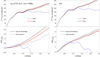 |
Fig. 1. SPT power spectra for the symmetron model (left panels) with assb = 0.33, m0 = 1 h/Mpc and β0 = 1, and for the F4 model (right panels), evaluated at redshift z = 0. We plot the linear theory, the full SPT, the SPT without screenings, and the SPT considering only S1 (source1) screenings (see text for details). In the lower panels we take their ratios to the one-loop SPT power spectrum for the ΛCDM model. |
5. Screening growth functions
In this section we study the main features of the normalized second- and third-order growth functions  and
and  . Since a Dirac delta function accompanies the second-order growth functions and ensures that k = k1 + k2, these three wave vectors form a triangle. Therefore, by assuming statistical homogeneity and isotropy, the growth functions depend only on three positive numbers, for example, the lengths of the sides of the triangles. We can therefore write
  . Three triangle configurations are considered: equilateral, k = k1 = k2; orthogonal,
  ; and squeezed, k ≃ k1, k2 ≃ 0. There is a second squeezed configuration with k ≃ 0 and k1 ≃ k2 corresponding to very large scales, where the fifth force vanishes for mass-less theories and the screenings are zero. Analogously, we consider third-order screening growths given by Eq. (42) in the doubled-squeezed configuration explained above.
We stress that  and
and  with positive values will screen the fifth force, while negative values will act anti-screening it instead. Given this, the M functions of each model will determine their screening properties.
5.1. Chameleon screening in the Jordan frame: the f(R) case
First, we consider the f(R) Hu-Sawicki model for different fR0 = −10−4, −10−8, −10−12 corresponding to the F4, F8, and F12 models. In the upper panel of Fig. 2 we show plots for the second-order screening growth functions,  , evaluated at redshift z = 0 and for different triangular configurations. The vertical lines correspond to the screening wave number
 (70)
(70)
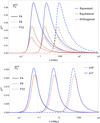 |
Fig. 2.
|


which provides us with a rough estimate to characterize the scale at which the screening is present; it is close to the maximum screening growth of the largest triangular contribution (squeezed modes). We note that in f(R), the screening scale has a simple dependence  , as can be seen from Eq. (50). The lower panel of Fig. 2 shows the growth
  for the double-squeezed configuration with additionally |k|=|p| and for different values of the cosine angle
  .
.
kM1 should be understood as a phenomenological scale that does not show where the screening effects start to be present, but its usefulness is that it characterizes the screening for the models considered in this work. To show this at different redshifts, we study the effects of the background evolution on the screening growth. In Fig. 3 we show this for the F4 model at different redshifts z = 0, 3, and 10. The upper panel uses a ΛCDM background cosmology and the lower panel an EdS background evolution. In ΛCDM the screening curves are narrower and reach smaller maxima. This is expected because the cosmic acceleration attenuates the clustering of dark matter, and hence the nonlinear effects. Instead, in an EdS background, the growth pattern is preserved and only shifted by the scale kM1 (denoted again by the vertical lines). Although this scale is useful, we note that it does not provide the range over which the screening growth is present. This will be more evident in the following section, where we study the symmetron model and show that the behavior of the growth is very different below and above kM1.
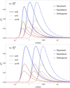 |
Fig. 3.
|


It is worthwhile to observe that in f(R), the nonlinearities of the Klein–Gordon equation lead to screening for any configuration. This is manifested in Figs. 2 and 3 because the screening growth functions always take positive values. To show this behavior, we show in Fig. 4 the second-order normalized growth functions  and
and  (upper panel) and their ratios (bottom panel) for the equilateral and orthogonal configurations. Because the ratios always take values lower than unity, the standard screening behavior always occurs. This a consequence of Eq. (51), which shows that M2 is always positive. Below we show that this is not necessarily the case for models defined in the Einstein frame.
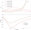 |
Fig. 4. Normalized second-order growth functions |


5.2. Symmetron screening
We consider the case of symmetron models. In Fig. 5 we show the second-order screening growth functions for models with  , assb = 0.33, and different values of m0 and β0. The vertical lines correspond again to the characteristic scale kM1. We are interested in also studying the growth functions at different redshifts, but since for
  the function M1 becomes a constant, the corresponding kM1 values are only rescaled by the scale factor. For this reason, we do it with a model with
  and
and  . The other parameters are fixed to assb = 0.33, m0 = 1 h Mpc−1, and β0 = 1. For this case, we show plots in Fig. 7.
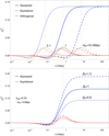 |
Fig. 5.
|


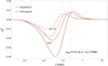 |
Fig. 7.
|


Unlike in f(R) theories, the nonlinear terms in the Klein–Gordon equation for symmetron models lead to anti-screening effects (negative regions of the plots, cf. Figs. 5 and 7), or more precisely, there are configurations of interacting wave modes that instead of driving the theory toward GR drive the theory away from it. From Eq. (37), all triangular configurations with
 (71)
(71)
where the anti-screening wave number is defined as
 (72)
(72)
will contribute with a negative source to the second-order screening as long as the RHS of the above equation is positive. We note that for the symmetron model, the anti-screening effects appear at scales below kM1, although there is no a priori evident reason for this to happen, and it might be the case that other Einstein-frame posited theories show anti-screening effects above kM1 as well.
In Fig. 6 we show an equivalent plot to Fig. 4, where in the upper panel we show the growth functions  and
and  , and in the lower panel we present their ratio. Regions where the ratios are greater than 1 correspond to wave-number configurations that act as anti-screening, that is, that enhance the MG fifth force.
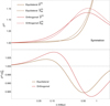 |
Fig. 6. Normalized second-order growth functions |


The situation is similar when we consider third-order screening growth functions  , as shown in Fig. 8. We again note that while f(R) models always lead to positive screenings, symmetron models pose configurations that enhance the MG fifth force.
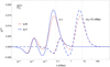 |
Fig. 8. Third-order growth function |

We may think of the case of the (original) chameleons (Khoury & Weltman 2004b) defined in the Einstein frame. Here we have a conformal factor C(φ) = eφ/M ≃ 1 + φ/M and a potential V(φ) that decays with the scalar field. The linear conformal coupling implies that functions βn vanish for n ≥ 2 (or at least, if we consider the full coupling eφ/M, they are quite small compared to β) and by virtue of Eqs. (27) and (28), the functions M2 and M3 become scale independent. Moreover, the effective mass in these models decays with time, implying that function κ3(a) is negative, while function κ4(a) is positive. Then M2 and M3 are always positive. Hence, the growth functions will have the same kind of behavior as we observe in f(R). Equivalently, this can be observed at second order from the anti-screening wavenumber in Eq. (72), which is always negative, and hence no scale contributes to anti-screening configurations. In contrast to this, in symmetron models the effective mass grows with time and therefore κ3 is positive, but β2 is different from zero because the conformal coupling is quadratic in the scalar field. Henceforth, we observe this mix of screening and anti-screenings effects in PT.
5.3. Vainshtein screening: the DGP case
The source  in Eq. (37) for the DGP and cubic Galileons depends only on the angle
  of the triangle configuration, and not on the scales k and p. This is because the mass of the scalar field is zero in these cases. By combining Eqs. (37) and (54), we obtain
 (73)
(73)
where we note that the linear growth D+(a) is also scale independent.
In Fig. 9 we show  for the normal branch DGP with a cross-over scale equal to the Hubble size,
  . For both cubic Galileons and DGP, it is a function depending only on x and time.
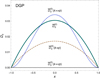 |
Fig. 9.
|


On the other hand, the symmetrized M3 function, again in the double-squeezed configuration, becomes
![Mathematical equation: $$ \begin{aligned} M_3(\mathbf{k },-\mathbf{p },\mathbf{p }) = \frac{Z_1(a)}{2 a^2 \beta ^4(a) A_0}[k^2 p^4 (1-x^2) - k^3 p^3 x(1-x^2)]. \end{aligned} $$](/articles/aa/full_html/2019/02/aa34383-18/aa34383-18-eq149.gif) (74)
(74)
Because the second term on the RHS of the above equation is odd in x, it does not contribute when D(3) is integrated in Eq. (63) to obtain loop statistics. Hence we do not consider it here. The third-order screening growth  does depend on the scale, but only through the ratio p/k. In Fig. 9 we show this dependence for p = k and the limiting cases p ≫ k and p ≪ k.
We observe that the second- and third-order screening growths always act to attenuate the fifth force that modifies Newtonian gravity.
Recently, Ogawa et al. (2018) found matter configurations that yielded anti-screening responses in the cubic Galileon model. In PT we found that these are absent, at least up to third order in matter fluctuations.
6. Conclusions
We presented a formalism for studying screening mechanisms in modified theories of gravity through perturbative methods. We redefined the scalar degree of freedom, which permitted us to recast the Einstein frame perturbation equations to the Jordan frame, for which we have at hand a previously developed theory for matter clustering in MG, which we were then able to apply. Although screening mechanisms are nonlinear phenomena, our perturbative approach gave us an analytical tool to probe and understand features in screening mechanisms. This allowed us to compare several theoretical models and to identify features that can be used to distinguish among them through their screening mechanisms.
An interesting result we obtained is that the perturbative screenings do not always act in the “screening direction”; that is, although the symmetron power spectrum, when considering only the source 𝒮1 in Eq. (69), contributes less to the screening than the full-loop curves, they are actually closer to the GR power spectrum, as shown in Fig. 1. The reason for this behavior lies in the nonlinearities of the Klein–Gordon equation in which the couplings provide anti-screening effects, among other effects.
We identified the emergence of a natural screening wave number,  , for weak coupling and high-mass screening models that served us to identify a scale of appearance of the screenings effects, as shown in Figs. (2–7). Although this represents only an approximate number, it could be useful for a rapid identification of screening occurrence.
Our computations show that in f(R) theories, the nonlinearities of the Klein–Gordon equation lead to screening for any configuration because the screening growing functions always take positive values. Unlike f(R) theories, the nonlinear terms in the Klein–Gordon equation for symmetron models lead to anti-screening effects. That is, there are configurations of interacting wave modes that instead of driving the theory toward General Relativity, drive the theory away from it. We traced this behavior back to both the quadratic conformal coupling and the effective mass of the theory that grows with time. In contrast, for the standard chameleon defined in the Einstein frame, the conformal factor is linear in the scalar field and its mass decays with time; as a result, the screening features of this model are qualitatively the same as those in f(R) theories. On the other hand, for the DGP and cubic Galileon models, we find no signatures of anti-screening up to third order in perturbation theory. Moreover, their second-order growth functions become trivial as they do not depend on the size of the triangle configurations, but only on one of the angles that define them. That is, they become scale independent, which we note is a consequence of the vanishing mass in these models.
Screening mechanisms leave imprints on the quasi-nonlinear matter power spectra that may represent a way to distinguish different gravity theories that otherwise behave in a very similar way at background and linear cosmological levels. Our present study indicates where to find the most probable of the different screening models within MG theories. This is especially important for validating MG N-body simulations with theory to later compare with forthcoming precision data from large-scale galaxy surveys such as eBOSS, DESI, EUCLID, and LSST.
We use the notation ∇x = ∂/∂x for derivatives with respect to Eulerian coordinates. For spatial Lagrangian coordinate derivatives, we use ∇ = ∂/∂q.
We adopt the shorthand notations
 (22)
(22)
and k1⋯n = k1 + ⋯ + kn.
Starting from Eq. (13), we use  . Afterward, we can expand (J−1)ij = δij − Ψi, j + Ψi, kΨk, j + ⋯.
Acknowledgments
DFM thanks the Research Council of Norway for their support, and the resources provided by UNINETT Sigma2 – the National Infrastructure for High Performance Computing and Data Storage in Norway. This paper is based upon work from the COST action CA15117 (CANTATA), supported by COST (European Cooperation in Science and Technology). JLCC and AA acknowledge financial support by the Consejo Nacional de Ciencia y Tecnología (CONACyT), Mexico, under grants 283151 and the Fronteras Project 281.
References
- Aghamousa, A., Aguilar, J., & Ahlen, S. 2016, ArXiv e-prints [arXiv:1611.00036] [Google Scholar]
- Akrami, Y., Koivisto, T. S., Mota, D. F., & Sandstad, M. 2013, JCAP, 1310, 046 [NASA ADS] [CrossRef] [Google Scholar]
- Amendola, L., & Tsujikawa, S. 2010, Dark Energy: Theory and Observations (Cambridge: Cambridge University Press) [Google Scholar]
- Amendola, L., Appleby, S., Bacon, D., et al. 2013, Liv. Rev. Rel., 16, 6 [Google Scholar]
- Aviles, A., & Cervantes-Cota, J. L. 2017, Phys. Rev. D, 96, 123526 [NASA ADS] [CrossRef] [Google Scholar]
- Aviles, A., Rodriguez-Meza, M. A., De-Santiago, J., & Cervantes-Cota, J. L. 2018, JCAP, 11, 013 [NASA ADS] [CrossRef] [Google Scholar]
- Babichev, E., Deffayet, C., & Ziour, R. 2009, Int. J. Mod. Phys. D, 18, 2147 [NASA ADS] [CrossRef] [Google Scholar]
- Babichev, E., Deffayet, C., & Esposito-Farèse, G. 2011, Phys. Rev. D, 84, 061502 [NASA ADS] [CrossRef] [Google Scholar]
- Baker, T., Psaltis, D., & Skordis, C. 2015, ApJ, 802, 63 [NASA ADS] [CrossRef] [Google Scholar]
- Barreira, A., Li, B., Hellwing, W. A., Baugh, C. M., & Pascoli, S. 2013, JCAP, 10, 027 [NASA ADS] [CrossRef] [Google Scholar]
- Barrow, J. D., & Mota, D. F. 2003, Class. Quant. Grav., 20, 2045 [NASA ADS] [CrossRef] [Google Scholar]
- Baumann, D., Nicolis, A., Senatore, L., & Zaldarriaga, M. 2012, JCAP, 1207, 051 [NASA ADS] [CrossRef] [Google Scholar]
- Bellini, E., & Zumalacarregui, M. 2015, Phys. Rev. D, 92, 063522 [NASA ADS] [CrossRef] [Google Scholar]
- Bertotti, B., Iess, L., & Tortora, P. 2003, Nature, 425, 374 [NASA ADS] [CrossRef] [PubMed] [Google Scholar]
- Bose, B., & Koyama, K. 2016, JCAP, 1608, 032 [Google Scholar]
- Bose, B., & Koyama, K. 2017, JCAP, 1708, 029 [NASA ADS] [CrossRef] [Google Scholar]
- Bose, B., & Taruya, A. 2018, JCAP, 1810, 019 [NASA ADS] [CrossRef] [Google Scholar]
- Bose, B., Koyama, K., Lewandowski, M., Vernizzi, F., & Winther, H. A. 2018, JCAP, 1804, 063 [NASA ADS] [CrossRef] [Google Scholar]
- Bouchet, F. R., Colombi, S., Hivon, E., & Juszkiewicz, R. 1995, A&A, 296, 575 [NASA ADS] [Google Scholar]
- Brax, P. 2013, Class. Quant. Grav., 30, 214005 [NASA ADS] [CrossRef] [Google Scholar]
- Brax, P., & Davis, A.-C. 2015, JCAP, 10, 042 [NASA ADS] [CrossRef] [Google Scholar]
- Brax, P., & Valageas, P. 2013, Phys. Rev. D, 88, 023527 [NASA ADS] [CrossRef] [Google Scholar]
- Brax, P., Davis, A.-C., Li, B., & Winther, H. A. 2012, Phys. Rev. D, 86, 044015 [NASA ADS] [CrossRef] [Google Scholar]
- Brax, P., van de Bruck, C., Davis, A.-C., Li, B., & Shaw, D. J. 2011, Phys. Rev. D, 83, 104026 [NASA ADS] [CrossRef] [Google Scholar]
- Bull, P., Akrami, Y., Adamek, J., et al. 2016, Phys. Dark Univ., 12, 56 [Google Scholar]
- Carlson, J., Reid, B., & White, M. 2013, MNRAS, 429, 1674 [NASA ADS] [CrossRef] [Google Scholar]
- Clampitt, J., Cai, Y.-C., & Li, B. 2013, MNRAS, 431, 749 [NASA ADS] [CrossRef] [Google Scholar]
- Clifton, T., Mota, D. F., & Barrow, J. D. 2005, MNRAS, 358, 601 [NASA ADS] [CrossRef] [Google Scholar]
- Clifton, T., Ferreira, P. G., Padilla, A., & Skordis, C. 2012, Phys. Rep., 513, 1 [NASA ADS] [CrossRef] [MathSciNet] [Google Scholar]
- Damour, T., & Polyakov, A. 1994, Nucl. Phys. B, 423, 532 [NASA ADS] [CrossRef] [MathSciNet] [Google Scholar]
- Davis, A.-C., Li, B., Mota, D. F., & Winther, H. A. 2012, ApJ, 748, 61 [NASA ADS] [CrossRef] [Google Scholar]
- Dvali, G., Gabadadze, G., & Porrati, M. 2000, Phys. Lett. B, 485, 208 [NASA ADS] [CrossRef] [MathSciNet] [Google Scholar]
- Fasiello, M., & Vlah, Z. 2017, Phys. Lett. B, 773, 236 [NASA ADS] [CrossRef] [Google Scholar]
- Gronke, M. B., Llinares, C., & Mota, D. F. 2014, A&A, 562, A9 [NASA ADS] [CrossRef] [EDP Sciences] [Google Scholar]
- Gronke, M., Llinares, C., Mota, D. F., & Winther, H. A. 2015, MNRAS, 449, 2837 [NASA ADS] [CrossRef] [Google Scholar]
- Hellwing, W. A., Cautun, M., Knebe, A., Juszkiewicz, R., & Knollmann, S. 2013, JCAP, 10, 012 [NASA ADS] [CrossRef] [Google Scholar]
- Hinterbichler, K., & Khoury, J. 2010, Phys. Rev. Lett., 104, 231301 [NASA ADS] [CrossRef] [Google Scholar]
- Hirano, S., Kobayashi, T., Tashiro, H., & Yokoyama, S. 2018, Phys. Rev. D, 97, 103517 [NASA ADS] [CrossRef] [Google Scholar]
- Hu, W., & Sawicki, I. 2007, Phys. Rev. D, 76, 064004 [CrossRef] [Google Scholar]
- Joyce, A., Jain, B., Khoury, J., & Trodden, M. 2015, Phys. Rept., 568, 1 [Google Scholar]
- Khoury, J., & Weltman, A. 2004a, Phys. Rev. D, 69, 044026 [CrossRef] [Google Scholar]
- Khoury, J., & Weltman, A. 2004b, Phys. Rev. Lett., 93, 171104 [NASA ADS] [CrossRef] [PubMed] [Google Scholar]
- Koyama, K. 2016, Rept. Prog. Phys., 79, 046902 [NASA ADS] [CrossRef] [Google Scholar]
- Koyama, K., Taruya, A., & Hiramatsu, T. 2009, Phys. Rev. D, 79, 123512 [NASA ADS] [CrossRef] [Google Scholar]
- LIGO Collaboration & Virgo Collaboration 2016, Phys. Rev. Lett., 116, 221101 [NASA ADS] [CrossRef] [PubMed] [Google Scholar]
- Llinares, C., & Mota, D. F. 2013, Phys. Rev. Lett., 110, 151104 [NASA ADS] [CrossRef] [Google Scholar]
- Lombriser, L., Schmidt, F., Baldauf, T., et al. 2012, Phys. Rev. D, 85, 102001 [NASA ADS] [CrossRef] [Google Scholar]
- Lombriser, L., Simpson, F., & Mead, A. 2015, Phys. Rev. Lett., 114, 251101 [NASA ADS] [CrossRef] [PubMed] [Google Scholar]
- LSST Dark Energy Science Collaboration 2012, ArXiv e-prints [arXiv:1211.0310] [Google Scholar]
- Martino, M. C., & Sheth, R. K. 2009, ArXiv e-prints [arXiv:0911.1829] [Google Scholar]
- Matsubara, T. 2008a, Phys. Rev. D, 77, 063530 [NASA ADS] [CrossRef] [Google Scholar]
- Matsubara, T. 2008b, Phys. Rev. D, 77, 063530 [NASA ADS] [CrossRef] [Google Scholar]
- Matsubara, T. 2008c, Phys. Rev. D, 78, 083519, Erratum: Phys. Rev. D78,109901(2008) [NASA ADS] [CrossRef] [Google Scholar]
- Matsubara, T. 2015, Phys. Rev. D, 92, 023534 [NASA ADS] [CrossRef] [Google Scholar]
- Nicolis, A., Rattazzi, R., & Trincherini, E. 2009, Phys. Rev. D, 79, 064036 [NASA ADS] [CrossRef] [MathSciNet] [Google Scholar]
- Ogawa, H., Hiramatsu, T., & Kobayashi, T. 2018, ArXiv e-prints [arXiv:1802.04969] [Google Scholar]
- Olive, K. A., & Pospelov, M. 2008, Phys. Rev. D, 77, 043524 [NASA ADS] [CrossRef] [Google Scholar]
- Oyaizu, H., Lima, M., & Hu, W. 2008, Phys. Rev. D, 78, 123524 [NASA ADS] [CrossRef] [Google Scholar]
- Perlmutter, S., Aldering, G., Goldhaber, G., et al. 1999, ApJ, 517, 565 [NASA ADS] [CrossRef] [Google Scholar]
- Pietroni, M. 2005, Phys. Rev. D, 72, 043535 [NASA ADS] [CrossRef] [Google Scholar]
- Riess, A. G., Filippenko, A. V., Challis, P., et al. 1998, AJ, 116, 1009 [NASA ADS] [CrossRef] [Google Scholar]
- Schmidt, F., Lima, M., Oyaizu, H., & Hu, W. 2009, Phys. Rev. D, 79, 083518 [NASA ADS] [CrossRef] [Google Scholar]
- Shirata, A., Shiromizu, T., Yoshida, N., & Suto, Y. 2005, Phys. Rev. D, 71, 064030 [NASA ADS] [CrossRef] [Google Scholar]
- Stark, A., Miller, C. J., Kern, N., et al. 2016, Phys. Rev. D, 93, 084036 [NASA ADS] [CrossRef] [Google Scholar]
- Taruya, A. 2016, Phys. Rev. D, 94, 023504 [NASA ADS] [CrossRef] [Google Scholar]
- Taruya, A., Koyama, K., Hiramatsu, T., & Oka, A. 2014a, Phys. Rev. D, 89, 043509 [NASA ADS] [CrossRef] [Google Scholar]
- Taruya, A., Nishimichi, T., Bernardeau, F., Hiramatsu, T., & Koyama, K. 2014b, Phys. Rev. D, 90, 123515 [NASA ADS] [CrossRef] [Google Scholar]
- Tassev, S. 2014, JCAP, 1406, 008 [NASA ADS] [CrossRef] [Google Scholar]
- Vainshtein, A. I. 1972, Phys. Lett., B, 39, 393 [Google Scholar]
- Vlah, Z., Seljak, U., & Baldauf, T. 2015a, Phys. Rev. D, 91, 023508 [NASA ADS] [CrossRef] [Google Scholar]
- Vlah, Z., White, M., & Aviles, A. 2015b, JCAP, 1509, 014 [NASA ADS] [CrossRef] [Google Scholar]
- Will, C. M. 2006, Liv. Rev. Rel., 9, 3 [Google Scholar]
- Will, C. M. 2014, Liv. Rev. Rel., 17, 4 [Google Scholar]
- Williams, J. G., Turyshev, S. G., & Boggs, D. H. 2004, Phys. Rev. Lett., 93, 261101 [NASA ADS] [CrossRef] [PubMed] [Google Scholar]
- Wyman, M., Jennings, E., & Lima, M. 2013, Phys. Rev. D, 88, 084029 [NASA ADS] [CrossRef] [Google Scholar]
- Zhao, G.-B. 2014, ApJS, 211, 23 [NASA ADS] [CrossRef] [Google Scholar]
- Zhao, G.-B., et al. 2016, MNRAS, 457, 2377 [NASA ADS] [CrossRef] [Google Scholar]
Appendix A: Third-order growth functions
In this appendix we display the sources of the third-order growth function D(3)s(k, −p, k) differential equation of Eq. (69). First we define the normalized second-order growth of matter fluctuations
 (A.1)
(A.1)
with  and
and  solutions to Eqs. (36) and (37). We also use the growth function for the scalar field χ,
 (A.2)
(A.2)
with the frame-lagged  function
 (A.3)
(A.3)
The sources of Eq. (69) are given by
 (A.4)
(A.4)
![Mathematical equation: $$ \begin{aligned} \mathcal{S} _2&= - D_+(p)\left(A(p) + A(|\mathbf{k }+ \mathbf{p }|) - 2A(k)\right) D^{(2)}(\mathbf{p },\mathbf{k }) \nonumber \\ *&+ \left(2A(k) - A(p) - A(|\mathbf{k }+ \mathbf{p }|) \right) D_+(k) D_+^2(p) \frac{(\mathbf{k }\cdot \mathbf{p })^2}{k^2p^2} \nonumber \\&- \left( A(|\mathbf{k }+ \mathbf{p }|) - A(k) \right) D_+(k) D_+^2(p) - \left[ \frac{M_1(\mathbf{k }+ \mathbf{p })}{3\Pi (|\mathbf{k }+ \mathbf{p }|)} \mathcal{K} ^{(2)}_{\mathrm{FL} }(\mathbf{p },\mathbf{k })\right. \nonumber \\&\left. - \left(\frac{2 A_0}{3}\right)^2 \frac{M_2(\mathbf{p },\mathbf{k }) |\mathbf{k }+ \mathbf{p }|^2/a^2}{6\Pi (|\mathbf{k }+ \mathbf{p }|)\Pi (k)\Pi (p)} \right] D_+(k) D_+^2(p) \end{aligned} $$](/articles/aa/full_html/2019/02/aa34383-18/aa34383-18-eq161.gif) (A5)
(A5)
![Mathematical equation: $$ \begin{aligned}&(A(p) - A_0) D^{(2)}(\mathbf{p },\mathbf{k }) D_+(p) +\left( 2 \frac{(\mathbf{p }\cdot (\mathbf{k }+ \mathbf{p }))^2}{p^2 |\mathbf{p }+\mathbf{k }|^2} - \frac{\mathbf{p }\cdot (\mathbf{k }+\mathbf{p })}{|\mathbf{k }+\mathbf{p }|^2}\right) \nonumber \\&\times (A(|\mathbf{k }+\mathbf{p }|) - A_0) D^{(2)}_\chi (\mathbf{p },\mathbf{k }) D_+(p) + \nonumber \\&\left. 3 \frac{(\mathbf{k }\cdot \mathbf{p })^2}{k^2 p^2} \left( A(k) + A(p) - 2 A_0 \right) D_+(k) D_+^2(p) \right] + (\mathbf{p }\rightarrow -\mathbf{p }), \end{aligned} $$](/articles/aa/full_html/2019/02/aa34383-18/aa34383-18-eq163.gif) (A6)
(A6)
 (A7)
(A7)
with the third-order kernel of screenings
![Mathematical equation: $$ \begin{aligned}&\mathcal{K} _{\delta I}^{(3)s} (\mathbf{k },-\mathbf{p },\mathbf{p }) = 2\left(\frac{2A_0}{3}\right)^2 \frac{M_2(\mathbf{k },0)}{\Pi (k)\Pi (0)} \nonumber \\&+ \frac{(2A_0/3)^3}{3\Pi ^2(p)\Pi (k)} \left[M_3(\mathbf{k },-\mathbf{p },\mathbf{p }) - \frac{M_2(\mathbf{k },0)M_2^\mathrm{FL} (-\mathbf{p },\mathbf{p })}{\Pi (0)} \right] \nonumber \\&+\left(\frac{2A_0}{3}\right)^2 \frac{M_2(-\mathbf{p },\mathbf{k }+\mathbf{p })}{\Pi (k)\Pi (|\mathbf{k }+\mathbf{p }|)} \left(1+(\hat{\mathbf{k }}\cdot \hat{\mathbf{p }})^2 + \frac{D^{(2)}(\mathbf{p },\mathbf{k })}{D_+(p)D_+(k)} \right)\nonumber \\&+ \frac{(2A_0/3)^3}{3\Pi ^2(p)\Pi (k)} \left[M_3(\mathbf{k },-\mathbf{p },\mathbf{p }) - \frac{M_2(-\mathbf{p },\mathbf{k }+\mathbf{p })M_2^\mathrm{FL} (\mathbf{k },\mathbf{p })}{\Pi (|\mathbf{k }+\mathbf{p }|)} \right]\nonumber \\&+\left(\frac{2A_0}{3}\right)^2 \frac{M_2(\mathbf{p },\mathbf{k }-\mathbf{p })}{\Pi (k)\Pi (|\mathbf{k }-\mathbf{p }|)} \left(1+(\hat{\mathbf{k }}\cdot \hat{\mathbf{p }})^2 + \frac{D^{(2)}(-\mathbf{p },\mathbf{k })}{D_+(p)D_+(k)} \right)\nonumber \\&+ \frac{(2A_0/3)^3}{3\Pi ^2(p)\Pi (k)} \left[M_3(\mathbf{k },-\mathbf{p },\mathbf{p }) - \frac{M_2(\mathbf{p },\mathbf{k }-\mathbf{p })M_2^\mathrm{FL} (\mathbf{k },-\mathbf{p })}{\Pi (|\mathbf{k }-\mathbf{p }|)} \right]. \end{aligned} $$](/articles/aa/full_html/2019/02/aa34383-18/aa34383-18-eq165.gif) (A.8)
(A.8)
We note that these functions are valid for symmetrized M2 and M3 functions.
All Figures
|
Fig. 1. SPT power spectra for the symmetron model (left panels) with assb = 0.33, m0 = 1 h/Mpc and β0 = 1, and for the F4 model (right panels), evaluated at redshift z = 0. We plot the linear theory, the full SPT, the SPT without screenings, and the SPT considering only S1 (source1) screenings (see text for details). In the lower panels we take their ratios to the one-loop SPT power spectrum for the ΛCDM model. |
| In the text | |
|
Fig. 2.
|
| In the text | |
|
Fig. 3.
|
| In the text | |
|
Fig. 4. Normalized second-order growth functions |
| In the text | |
|
Fig. 5.
|
| In the text | |
|
Fig. 7.
|
| In the text | |
|
Fig. 6. Normalized second-order growth functions |
| In the text | |
|
Fig. 8. Third-order growth function |
| In the text | |
|
Fig. 9.
|
| In the text | |
Current usage metrics show cumulative count of Article Views (full-text article views including HTML views, PDF and ePub downloads, according to the available data) and Abstracts Views on Vision4Press platform.
Data correspond to usage on the plateform after 2015. The current usage metrics is available 48-96 hours after online publication and is updated daily on week days.
Initial download of the metrics may take a while.