© ESO 2019

1. Introduction

Low Mach number flows sometimes appear in astrophysical phenomena. One typical example is the stellar convection zone, where the Mach number is very small (∼10⁻³ or less). In such cases, the time step criterion for explicit methods is severely limited by the fast speed of sound via the Courant-Friedrich-Lewy (CFL) condition, even if we are interested in the much slower dynamics of convective motion. Various numerical methods are suggested for efficient simulation of low Mach number flows (see Kupka & Muthsam 2017, for a review of the numerical modeling of the stellar convection).

One major way to simulate low Mach number flows is to assume that the speed of sound is infinite, as is done in the Boussinesq/anelastic approximations (e.g., Miesch et al. 2008). The drawback of these methods is the necessity of global communication in parallel computing. A sound wave with infinite speed forces the entire computational domain to interact instantaneously. Implicit time integration of the sound wave as in the stratified approximation (Chan et al. 1994; Cai 2016) also suffers from this difficulty. This characteristic can be a source that prevents high parallel computing efficiency in a numerical simulation.

The reduced speed of sound technique (RSST) was first developed to compute the steady-state solution (Rempel 2005) and was extended to the thermal convection problem (Hotta et al. 2012). In the RSST, speed of sound is artificially reduced by a free parameter ξ so that the severe time step criterion due to a fast speed of sound can be relaxed. The equations are fully explicit and can be easily implemented with parallel computers using domain decomposition. Hotta et al. (2015) also suggested an invariant that exhibits better conservation properties. The RSST has been previously applied to solar and stellar convection problems with and without magnetic fields (Hotta et al. 2014, 2015, 2016; Käpylä et al. 2016). In contrast to the high Reynolds number in stellar convection, mantle convection in the Earth has a very low Reynolds number. Takeyama et al. (2017) proposed a method to solve such problems using a strategy that is similar to RSST. In the following, we concentrate on applications to high Reynolds number flows.

One limitation of the original RSST is that it was formulated and tested for problems where density perturbations are sufficiently smaller than the background density. As shown in Sects. 2 and 4, we find that the original version of the RSST cannot be used to handle low Mach number flows with large density variations. Large density variations in low Mach number flows sometimes appear in problems with the state equation for nonideal gases and/or nuclear or chemical reactions such as the convective phase of Type Ia supernova (Zingale et al. 2005; Glasner et al. 2007; Nonaka et al. 2010).

Another limitation of the original RSST is that the evolution equations for nonconservative variables (velocity field and specific entropy) must be solved. This limitation comes from the requirement that the evolution of the entropy equation be solved directly so that artificial reduction of the speed of sound does not affect the characteristics of the entropy wave. However, the conservative form is preferred when the solution includes discontinuities such as shock waves, especially in finite-difference and finite-volume schemes (Hou & Lefloch 1994). Let us take an example from stellar convection simulations, where the numerical domain extends from the deep stellar convection zone to the photosphere or upper atmosphere. The basic RSST equations in the deep convection zone do not reduce smoothly to the conservative equations used in surface convection simulations (Nordlund 1982; Stein & Nordlund 1989; Vögler et al. 2005; Iijima & Yokoyama 2015, 2017).

In this study, we suggest several new formulations to reduce the speed of sound while maintaining the properties of the entropy wave. The new methods have two advantages: First, they can be applied to flows with large density variation. Second, they evolve the conservative variables and reduce to the conservative Euler equations when the speed of sound is not reduced. These advantages of the newly suggested RSST methods lead to their application in a wide range of problems.

2. Original formulation of the reduced speed of sound technique (DVS form)

In this section, we summarize the original formulation of the RSST (Rempel 2005; Hotta et al. 2012) and show that this method cannot be applied to problems with large density variations. In this study, we call this original version of the RSST the DVS form (each abbreviation shows D: density, V: velocity, and S: entropy).

2.1. Reducing the time derivative of mass density

The original formulation of the RSST in Cartesian coordinates is formulated by dividing each variables into the background stratification and perturbation. The inviscid Euler equations with the RSST are given by

$$\begin{array}{cc}& {\xi }^2\frac{\partial {\rho }_1}{\partial t}+\mathrm{\nabla }·\left({\rho }_0\mathit{V}\right)=0\hfill \\ \hfill & \frac{\partial V_i}{\partial t}+\mathit{V}·\mathrm{\nabla }{V}_i+\frac{1}{{\rho }_0}\frac{\partial P_1}{\partial x_i}=0\hfill \\ \hfill & \frac{\partial S_1}{\partial t}+\mathit{V}·\mathrm{\nabla }(S_0+S_1)=0,\hfill \end{array}$$(1)

where ρ is the mass density, V is the velocity field, P is the gas pressure, S is the specific entropy, and i = x, y, z. The subscripts 0 and 1 denote the background stratification and perturbation, respectively. The perturbation is assumed to be small and the background stratification does not vary in time, i.e.,

$$\begin{array}{c}\hfill P_1\ll P_0,{\rho }_1\ll {\rho }_0,{\partial }_t{P}_0={\partial }_t{\rho }_0=0.\end{array}$$(2)

The important point is that the entropy equations are not altered by applying the RSST. This allows us to evolve flows without modifying the characteristics of the entropy wave. We assume that P₀ is spatially uniform in the above formulation. In a practical situation, the gradient of P₀ balances the external forces (e.g., the gravitational force). This difference does not affect the discussion in this paper.

We rewrite the original equations (Eq. (1)) without dividing by the background and perturbations in the variables, without changing the phase speed of each mode under the limit in Eq. (2). The resulting equations are given by

$$\begin{array}{cc}& {\xi }^2\frac{\partial \rho }{\partial t}+\mathrm{\nabla }·\left(\rho \mathit{V}\right)=0\hfill \\ \hfill & \frac{\partial V_i}{\partial t}+\mathit{V}·\mathrm{\nabla }{V}_i+\frac{1}{\rho }\frac{\partial P}{\partial x_i}=0\hfill \\ \hfill & \frac{\partial S}{\partial t}+\mathit{V}·\mathrm{\nabla }S=0,\hfill \end{array}$$(3)

where we assume the general equation of state P(ρ, S).

Let us consider a plane wave in the x-direction and analyze the phase speed of each wave mode. The one-dimensional version of Eq. (3) is given by

$$\begin{array}{cc}& {\xi }^2\frac{\partial \rho }{\partial t}+V_x\frac{\partial \rho }{\partial x}+\rho \frac{\partial V_x}{\partial x}=0\hfill \\ \hfill & \frac{\partial V_x}{\partial t}+V_x\frac{\partial V_x}{\partial x}+\frac{1}{\rho }\frac{\partial P}{\partial x}=0\hfill \\ \hfill & \frac{\partial S}{\partial t}+V_x\frac{\partial S}{\partial x}=0.\hfill \end{array}$$(4)

These equations can be rewritten as

$$\begin{array}{c}\hfill \begin{array}{cc}& \frac{\partial }{\partial t}\left(\begin{array}{c}\rho \\ V_x\\ S\end{array}\right)+A\frac{\partial }{\partial x}\left(\begin{array}{c}\rho \\ V_x\\ S\end{array}\right)=0\hfill \\ \hfill & A=\left(\begin{array}{ccc}1/{\xi }^2& 0& 0\\ 0& 1& 0\\ 0& 0& 1\\ \end{array}\right)\left(\begin{array}{ccc}{V}_x& \rho & 0\\ a^2/\rho & V_x& P_S/\rho \\ 0& 0& V_x\\ \end{array}\right)\hfill \\ \hfill & =\left(\begin{array}{ccc}{V}_x/{\xi }^2& \rho /{\xi }^2& 0\\ a^2/\rho & V_x& P_S/\rho \\ 0& 0& V_x\\ \end{array}\right),\hfill \end{array}\end{array}$$(5)

where P_S = (∂P/∂S)_ρ, and $a=\sqrt{{(\partial P/\partial \rho )}_S}$ is the adiabatic speed of sound. In the case of an ideal gas, (∂P/∂ρ)_S = γP/ρ and (∂P/∂S)_ρ = P/C_V, where γ is the specific heat ratio and C_V is the specific heat capacity at constant volume.

The phase speed of each wave mode is equal to an eigenvalue of the Jacobian A, which is given by

$$\begin{array}{c}\hfill \lambda =\{\begin{array}{c}{V}_x,\hfill \\ \frac{1}{2}[(1+\frac{1}{{\xi }^2})V_x\pm \sqrt{D}],\hfill \end{array}\end{array}$$(6)

where

$$\begin{array}{c}\hfill D={(1-\frac{1}{{\xi }^2})}^2{V}_x^2+4\frac{a^2}{{\xi }^2}·\end{array}$$(7)

Apparently, D >  0 is always satisfied and all eigenvalues are real, which indicates that the basic RSST equations in the DVS form (Eq. (3)) are hyperbolic. The first wave mode λ = V_x corresponds to the entropy wave. The other two wave modes correspond to right/left-propagating sound waves. When the Mach number is small enough (|V|≪C), the speed of the sound wave becomes λ ∼ ±a/ξ. Thus, the RSST can be used to reduce the speed of sound without affecting the characteristics of the entropy wave.

2.2. Drawback from reducing the time derivative of mass density

Although the original DVS form is simple and easy to implement, this approximation excites an artificial pressure perturbation when the density perturbation is not small compared to the background. From the RSST continuity and entropy equations in Eq. (3), we find that the equation describing evolution of the gas pressure is given by

$$\begin{array}{c}\hfill \frac{\partial P}{\partial t}+\mathit{V}·\mathrm{\nabla }P+\rho a^2\mathrm{\nabla }·\mathit{V}=(1-\frac{1}{{\xi }^2})a^2(\mathit{V}·\mathrm{\nabla }\rho +\rho \mathrm{\nabla }·\mathit{V}).\end{array}$$(8)

Let us assume a situation in which the velocity field is incompressible (i.e., ∇ ⋅ V = 0) and the gas pressure is uniform (i.e., ∇P = 0). Such a situation nearly occurs during the evolution of low Mach number flows because the gas pressure is adjusted by the fast sound wave until the forces balance each other. Equation (8) leads to

$$\begin{array}{c}\hfill \frac{\partial P}{\partial t}=(1-\frac{1}{{\xi }^2})a^2(\mathit{V}·\mathrm{\nabla }\rho ).\end{array}$$(9)

This means that density advection causes a pressure imbalance and excites artificial sound waves. This drawback is clearly shown in a Kelvin-Helmholtz instability test problem (Sect. 4.5). If the RSST is not used (i.e., ξ = 1), the pressure balance is maintained.

The RSST has been applied to the deep region of the stellar convection zone, where mass density perturbations are very small compared to the background density (∼10⁻⁴ or less). In such a case, the amplitude of the artificially excited pressure perturbation is negligible. However, the RSST would not be applicable to a situation with large density variations, which occurs in some astrophysical phenomena.

3. Reduced speed of sound technique for problems with large density variation (PVS form)

In this section, we propose a new RSST formulation named “PVS form” (P: pressure, V: velocity, and S: entropy) that is suitable for low Mach number flows with large density variations. In Sect. 3.1, we introduce the basic PVS form equations and we investigate their characteristics. In Sect. 3.2, we show that the PVS form can be rewritten in a semiconservative form so that conservative variables can be evolved directly. This is advantageous because the basic equations of the RSST become the conservative Euler equations when the speed of sound is not reduced (ξ = 1), which is suitable for solving systems that contain discontinuous phenomena such as shock waves.

3.1. Reducing the temporal evolution of gas pressure

The PVS form is a new formulation of the RSST based on equations describing the evolution of (P, V, S). In this formulation, we limit the time variation of the gas pressure instead of the mass density to reduce the speed of sound. The basic equations are given by

$$\begin{array}{cc}& {\xi }^2\frac{\partial P}{\partial t}+\mathit{V}·\mathrm{\nabla }P+\rho a^2\mathrm{\nabla }·\mathit{V}=0\hfill \\ \hfill & \frac{\partial V_i}{\partial t}+\mathit{V}·\mathrm{\nabla }{V}_i+\frac{1}{\rho }\frac{\partial P}{\partial x_i}=0\hfill \\ \hfill & \frac{\partial S}{\partial t}+\mathit{V}·\mathrm{\nabla }S=0.\hfill \end{array}$$(10)

Apparently, the new formulation in Eq. (10) maintains pressure equilibrium when the initial pressure is uniform and the divergence of the velocity field is zero. Equation (10) reduces the time variation of the pressure instead of reducing the density variation. We find this characteristic to be advantageous in more practical situations, such as those tested in Sect. 4.

Equation (10) have wave speeds that are identical to the wave speeds in the original DVS form. The one-dimensional version of Eq. (10) is given by

$$\begin{array}{cc}& \frac{\partial }{\partial t}\left(\begin{array}{c}P\\ V_x\\ S\end{array}\right)+A\frac{\partial }{\partial x}\left(\begin{array}{c}P\\ V_x\\ S\end{array}\right)=0,\hfill \end{array}$$(11)

where

$$\begin{array}{c}\hfill A=\left(\begin{array}{ccc}{V}_x/{\xi }^2& \rho a^2/{\xi }^2& 0\\ 1/\rho & V_x& 0\\ 0& 0& V_x\\ \end{array}\right).\end{array}$$(12)

The eigenvalues of the Jacobian A are given by

$$\begin{array}{cc}& \lambda =\{\begin{array}{c}{V}_x,\hfill \\ \frac{1}{2}[(1+\frac{1}{{\xi }^2})V_x\pm \sqrt{D}],\hfill \end{array}\hfill \end{array}$$(13)

where

$$\begin{array}{cc}& D={(1-\frac{1}{{\xi }^2})}^2{V}_x^2+4\frac{a^2}{{\xi }^2}·\hfill \end{array}$$(14)

The wave speeds λ are identical to the speeds in Eqs. (6) and (7). The new PVS form can also reduce the speed of sound without affecting the nature of the entropy wave, as is the case in the DVS form.

3.2. PVS form for conservative variables

The basic PVS form equations (Eq. (10)) can be rewritten in the semiconservative form as

$$\begin{array}{cc}& \frac{\partial \rho }{\partial t}+\mathrm{\nabla }·\left(\rho \mathit{V}\right)=-(1-\frac{1}{{\xi }^2}){\left(\frac{\partial \rho }{\partial P}\right)}_S\Delta P\hfill \\ \hfill & \frac{\partial }{\partial t}\left(\rho V_i\right)+\mathrm{\nabla }·\left(\rho V_i\mathit{V}\right)+\frac{\partial P}{\partial x_i}=-(1-\frac{1}{{\xi }^2}){\left(\frac{\partial \rho V_i}{\partial P}\right)}_{\mathit{V},S}\Delta P\hfill \\ \hfill & \frac{\partial E}{\partial t}+\mathrm{\nabla }·\left[(E+P)\mathit{V}\right]=-(1-\frac{1}{{\xi }^2}){\left(\frac{\partial E}{\partial P}\right)}_{\mathit{V},S}\Delta P,\hfill \end{array}$$(15)

where $E=e+\frac{1}{2}\rho V^2$ is the total energy density, and e(ρ, P) is the internal energy density (for the ideal equation of state, e = P/(γ − 1)). The partial derivatives on the right-hand side of Eq. (15) are given by

$$\begin{array}{c}\hfill {\left(\frac{\partial \rho }{\partial P}\right)}_S=\frac{1}{a^2},{\left(\frac{\partial \rho V_i}{\partial P}\right)}_{\mathit{V},S}=\frac{V_i}{a^2},{\left(\frac{\partial E}{\partial P}\right)}_{\mathit{V},S}=\frac{e+P+\rho V^2/2}{\rho a^2}·\end{array}$$(16)

The value ΔP is the time derivative of the gas pressure before reducing the speed of sound and is given by

$$\begin{array}{cc}\hfill \Delta P& =-\mathit{V}·\mathrm{\nabla }P-\rho a^2\mathrm{\nabla }·\mathit{V}\hfill \\ \hfill & =-{\left[{\left(\frac{\partial e}{\partial P}\right)}_{\rho }\right]}^{-1}\{[\frac{1}{2}{V}^2-{\left(\frac{\partial e}{\partial \rho }\right)}_P]\mathrm{\nabla }·\left(\rho \mathit{V}\right)\hfill \\ \hfill & -V_i[\mathrm{\nabla }·\left(\rho V_i\mathit{V}\right)+\frac{\partial P}{\partial x_i}]+\mathrm{\nabla }·\left[(E+P)\mathit{V}\right]\}.\hfill \end{array}$$(17)

The thermodynamic derivatives are given by

$$\begin{array}{c}\hfill {\left(\frac{\partial e}{\partial P}\right)}_{\rho }=\frac{\rho T}{P_S},{\left(\frac{\partial e}{\partial \rho }\right)}_P=\frac{e+P}{\rho }-\frac{\rho T{a}^2}{P_S}·\end{array}$$(18)

In the state equation for an ideal gas, (∂e/∂P)_ρ = 1/(γ−1) and (∂e/∂ρ)_P = 0. Equation (15) indicate that the speed of sound can be reduced as it was in the PVS form by adding a correction term to the right-hand side of the conservative Euler equations. This reduces the pressure variation while ensuring that variations in the specific entropy and velocity field are unchanged.

By solving Eq. (15), we can reduce the speed of sound without affecting the entropy wave. When the speed of sound is not reduced (i.e., ξ = 1), the equations reduce to the conservative Euler equations. Thus, the equations can be easily applied to problems with both shock waves and low Mach number flows.

Introducing new temporary variables

$$\begin{array}{cc}& \Delta \rho =-\mathrm{\nabla }·\left(\rho \mathit{V}\right)\hfill \\ \hfill & \Delta \left(\rho V_i\right)=-\mathrm{\nabla }·\left(\rho V_i\mathit{V}\right)-\frac{\partial P}{\partial x_i}\hfill \\ \hfill & \Delta E=-\mathrm{\nabla }·\left[(E+P)\mathit{V}\right].\hfill \end{array}$$(19)

Equations (15)–(18) can be rewritten as

$$\begin{array}{cc}& \frac{\partial \rho }{\partial t}=\Delta \rho -(1-\frac{1}{{\xi }^2}){\left(\frac{\partial \rho }{\partial P}\right)}_S\Delta P\hfill \\ \hfill & \frac{\partial }{\partial t}\left(\rho V_i\right)=\Delta \left(\rho V_i\right)-(1-\frac{1}{{\xi }^2}){\left(\frac{\partial \rho V_i}{\partial P}\right)}_{\mathit{V},S}\Delta P\hfill \\ \hfill & \frac{\partial E}{\partial t}=\Delta E-(1-\frac{1}{{\xi }^2}){\left(\frac{\partial E}{\partial P}\right)}_{\mathit{V},S}\Delta P,\hfill \end{array}$$(20)

where

$$\begin{array}{c}\hfill \Delta P={\left[{\left(\frac{\partial e}{\partial P}\right)}_{\rho }\right]}^{-1}\{[\frac{1}{2}{V}^2-{\left(\frac{\partial e}{\partial \rho }\right)}_P]\Delta \rho -V_i\Delta \left(\rho V_i\right)+\Delta E\}.\end{array}$$(21)

Equations (19)–(21) indicate that the proposed method can be easily implemented in existing numerical solvers for the conservative Euler equations by changing only the time derivatives (see also our implementation in Sect. 4.2). The additional computation is local and is suitable for use with the domain decomposition technique on parallel computers.

The steady solution (∂/∂t = 0) of the semiconservative form (Eq. (15)) is identical to the original Euler equations. This characteristic is apparent from Eqs. (19)–(21). This is advantageous not only for the steady problem, but also for quasi-steady problems such as thermal convection.

4. Test problems

4.1. Summary of the RSST variants

We summarize the newly suggested formulations of the RSST. In Sects. 2 and 3, we introduced the original DVS form of the RSST in nonconservative form and a new PVS form in semiconservative form, respectively. The DVS can be also rewritten in a semiconservative form, which is presented in Appendix A.1. We suggest two different formulations (PMS and DMS forms, where M stands for momentum) that employ the fully conservative momentum equations in Appendixes A.2 and A.3. We also construct another formulations (PD form; Appendix A.4) that uses the strict conservative forms in both mass and momentum equations. We note that the PD form does not satisfy the original form of the entropy equation.

In the test problem, we mainly focus on the PVS and PMS forms because they are based on a new idea to reduce the time evolution of the gas pressure. Although the PD form is also based on the idea of reducing the pressure variation, we do not focus on this form because it does not satisfy the entropy equation. However, in case of the required accuracy of the mass conservation is very severe, the PD form might perform well. The advantages and drawbacks of the PD form is described in Appendix A.4. We note here that the semiconservative forms of the DVS and DMS forms perform well in problems with small density variations, although we do not show the results explicitly in the current paper.

4.2. Numerical method

The proposed equations in the semiconservative form can be solved by the second-order MUSCL method (van Leer 1979). The monotonized-central limiter is used as a slope limiter. Temporal integration is carried out with the second-order strong stability preserving (SSP) Runge-Kutta method (Gottlieb et al. 2009). The local Lax-Friedrichs (LLF) scheme is used to compute the upwind numerical flux at the cell face. A Courant number of 0.4 is used for all test problems.

Several modifications are required to simulate the equations with the RSST. The characteristic speed used in the LLF scheme and the time step criterion must be changed to the maximum of the absolute eigenvalue of the corresponding RSST equations. In this study, we used an approximate characteristic speed c_tot = |V| + a/ξ for the LLF scheme, and the time step was computed for all proposed RSST forms. After the time derivatives are computed for each Runge-Kutta sub-step, the time derivatives are modified according to Eqs. (19)–(21) in the case of the PVS form. The RSST in other forms can be computed in a similar manner. Thus, the additional RSST computation is fully local and incurs only minor increases in numerical computational cost.

We summarize the implementation of the RSST (PVS form) in this study below.

1. Determine the size of time step using the CFL stability condition. Instead of using the maximum absolute value of exact wave speeds (Eqs. (6) and (7)), an approximate characteristic speed c_tot = |V| + a/ξ is used for simplicity.

2. Calculate limited slopes of the conservative variables.

3. Obtain left and right states at the cell interfaces based on the piecewise linear reconstruction.

4. Calculate numerical fluxes at the cell interfaces of the right-hand side of Eq. (19). We use the LLF scheme with a simplified characteristic speed c_tot = |V| + a/ξ.

5. Obtain divergence of numerical fluxes to get Δρ, Δ(ρV_i), and ΔE in Eq. (19).

6. Calculate ΔP using Eq. (21).

7. Calculate the time derivatives of conservative variables using Eq. (20).

8. Update the conservative variables by the Runge-Kutta method.

We note a more sophisticated way to implement the RSST in the upwind methods by using nonconservative variants of the path-conservative Riemann solver (Dumbser & Toro 2011; Dumbser & Balsara 2016). Because the RSST characteristics come from a modification of the basic equations, we believe that the qualitative characteristics of the results presented in this paper are independent from the choice of numerical method.

4.3. Functional form of the speed of sound reduction rate

There is some freedom for the functional form of the reduction rate of the speed of sound ξ. Hotta et al. (2012) suggested that a spatially nonuniform reduction rate can be also used in the RSST. In this study, we tested two different strategies to determine the reduction rate ξ.

The first strategy is to assume a spatially and temporally constant reduction rate ξ. This is easy to implement and interpret. The time step in this case is ξ times longer than the case without the RSST, if the Mach number is sufficiently low. The reduction rate ξ is roughly proportional to the speed increase in the simulations.

The second choice is to assume the speed of sound has an upper limit. Inspired by the choice of reduction rate of the Alfvén speed in Rempel et al. (2009), we use the functional form given by

$$\begin{array}{c}\hfill \xi ={[1+{(a/C_{\max })}^4]}^{1/4},\end{array}$$(22)

where C_max is the upper limit of the speed of sound. Eq. (22) gives the effective speed of sound

$$\begin{array}{c}\hfill a/\xi =a/{[1+{(a/C_{\max })}^4]}^{1/4}.\end{array}$$(23)

The effective speed of sound a/ξ approaches C_max when the speed of sound a increases. The choice of Eq. (22) can limit the speed of sound only when reduction of the speed of sound is necessary (i.e., when the speed of sound is similar or larger than the upper limit).

The second strategy is advantageous when the Mach number greatly varies in the numerical domain. For example, this applies in the solar/stellar surface convection simulation with the deep convection zone (e.g., Nordlund 1982). The numerical domain includes high Mach number shock waves with low speed of sound near the photosphere and low Mach number convection with high speed of sound. In this case, the numerical time step is sometimes limited by the high speed of sound in the deep convection zone and the semiconservative RSST can efficiently accelerate the simulation.

4.4. Linear wave convergence

We carry out a convergence analysis of the two-dimensional linear wave propagation (e.g., Gardiner & Stone 2005) to verify our implementation of the RSST code. We consider the entropy wave with velocity shear propagating at angle of θ = 30° relative to the x-axis. The computational domain size is [0, 1/cosθ]×[0, 1/sinθ] in the xy-plane. We use N × N grid points to resolve the domain with N = 16, 32, 64, 128, 256. The initial conditions are ρ = 1 + ϵsin(2πx_∥), P = 1000, V_∥ = 1, V_⊥ = ϵsin(2πx_∥), where x_∥ = xcosθ + ysinθ is the coordinate along the propagation direction of linear wave and ϵ = 10⁻⁵ is the wave amplitude. The subscripts ∥ and ⊥ represent the vector components parallel and orthogonal to the direction of wave propagation, respectively. The velocity components along the x and y axes are given by V_x = V_∥cosθ − V_⊥sinθ and V_y = V_∥sinθ + V_⊥cosθ, respectively. The specific heat ratio of 5/3 is used. The initial state is evolved for unit time (until t = 1). We assume a spatially and temporally uniform reduction rate ξ = 5 in this problem.

The L1 errors of the (normalized) specific entropy S = ln P − γlnρ, V_⊥, ρ, and P for each form of the RSST are shown in Fig. 1. The L1 error of each variable is defined as an volume averaged absolute value of the difference between the initial and final snapshots.

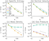Fig. 1. Convergence test of linear entropy wave. The horizontal axis N represents the number of grid points used in the x-direction. Shown are the L1 errors of the specific entropy (panel a), velocity component normal to the propagation direction of wave V⊥ (panel b), mass density (panel c), and gas pressure (panel d). Each line corresponds to the form of RSST used in the simulation. The dashed line in each panel shows the analytical line of second-order convergence. Details of the test problem are given in Sect. 4.4.

The entropy S and shear velocity V_⊥ (panels a and b in Fig. 1) exhibit second-order convergence in all forms of the RSST described in this paper. On the other hand, the gas pressure P (panel d) fails to converge in the DVS and DMS forms where the density variation is reduced. This is caused by the pressure variation caused by the advection of the nonuniform density (or entropy) as discussed in Sect. 2.2. With DVS and DMS forms, the error of the mass density ρ (panels c) shows weak convergence with the low resolution (N ≤ 32) but stagnates with higher resolution. When the pressure variation is reduced (PVS, PMS, and PD forms), the RSST exhibits second-order convergence with ρ and P. We note that, in more practical problems in which sound waves are produced in the numerical domain, even the PVS, PMS, and PD forms fail the convergence because the idea of reducing the speed of sound itself contains a source of error. However, we believe that the error from the basic idea remains at a tolerant level in many practical problems as shown in Sects. 4.5 and 4.6, and previous studies (e.g., Hotta et al. 2012).

The above result suggests that our numerical implementation of the RSST can reproduce the characteristics of the designed equations. The second-order convergence is achieved when the evolution equations of the variables are not altered by the RSST (e.g., entropy and shear velocity). In the following subsections, we apply the newly suggested forms of RSST for more complex and practical problems.

4.5. Two-dimensional Kelvin-Helmholtz instability

The two-dimensional Kelvin-Helmholtz instability in the low Mach number regime can reveal the applicability of our new RSST to complex flow structures in nearly uniform gas pressure. We employ a version of the problem suggested by McNally et al. (2012). The ideal equation of state was used with the specific heat ratio of 5/3 in all runs. Each run is computed with a resolution of 1024 × 1024 grids. We also carry out a high-resolution run with 4096 × 4096 grids without applying the RSST as a reference solution if necessary.

First, we investigate the Kelvin-Helmholtz instability in terms of the dependence on the initial density contrast ρ₂/ρ₁ to clarify the difference between the newly suggested PVS/PMS forms and the original DVS form (and a similar DMS form). We set ρ₁ = 1.0, and the gas pressure was set to 250 as a test problem for low Mach number flows. The speed of sound reduction rate ξ was fixed to 3. A typical Mach number without the RSST is about 0.04 in this problem.

One of the advantages of our new method based on the reduction of pressure evolution (PVS/PMS forms) over the original DVS form is its applicability to flows with high density contrast. Figure 2 demonstrates how the PVS and DVS forms work in the Kelvin-Helmholtz instability with different density contrasts. We compare the cases with different density contrasts of ρ₂/ρ₁ = 1.5 and 1.001. When the density contrast is small (ρ₂/ρ₁ = 1.001; bottom row), both PMS and DVS forms work well. However, with larger density contrast of ρ₂/ρ₁ = 1.5 (top row), the DVS form does not reproduce the vortex structure. The result demonstrates that the original DVS form can handle low Mach number flows only when the density variation is sufficiently small. This result is expected from the discussion in Sect. 2.2. The PVS form succeeds reproducing the correct time evolution, both with low and high density contrast. Although it is not shown in the plot, the results with the DMS form also demonstrate a similar drawback as the DVS form. The PMS form performs very similar to the PVS form. These results clarify the advantage of reducing the time evolution of the gas pressure in the RSST.

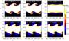Fig. 2. Snapshots from the Kelvin-Helmholtz instability with low density contrast at time = 1.5. The normalized density variation Δρ/Δρ0 = (ρ − ρ1)/(ρ2 − ρ1) is shown. Top row: results with density contrast of 1.5. Bottom row: results with density contrast of 1.001. Each column corresponds to a different reduction method for the speed of sound: without the RSST (ξ = 1; panels a and d), with the PVS form (ξ = 3; panels b and e), and with the DVS form (ξ = 3; panels c and f). Details of the test problem are given in Sect. 4.5.

Next, we focus on the newly suggested PVS/PMS forms and investigate the dependence on the reduction rate of the speed of sound. We set ρ₁ = 1.0,  ρ₂ = 2.0, and the gas pressure was set to 1000. A typical Mach number without the RSST is about 0.02 in this case.

Figure 3 shows the density structure of the Kelvin-Helmholtz instability at time = 1.5 with density contrast of 2. The spatial structure of the density without the RSST (panels a and d) is successfully reproduced by the PVS form (panels c and f) and PMS form (panels c and f). Both reduction rate choices (ξ-constant or C_max-constant) exhibit nearly identical density.

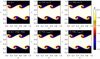Fig. 3. Snapshots of the Kelvin-Helmholtz instability with density contrast of 2 at time = 1.5. The color contour shows the mass density without the RSST (ξ = 1; panel a), with the PVS form (ξ = 10; panel b), with the PMS form (ξ = 10; panel c), without the RSST (ξ = 1) in 4096 × 4096 grids (panel d), with the PVS form (Cmax = 3; panel e), and with the PMS form (Cmax = 3; panel f). The detail of the test problem is shown in Sect. 4.5.

We note that the sharpness of the vortex is enhanced by using the RSST in Fig. 3 and is rather similar to the high-resolution run (panel d). This is caused by reduction of the characteristic speed, which is proportional to the numerical diffusion in the LLF scheme used in this study. The combination of RSST with the LLF scheme is an efficient choice for high-resolution simulation of low Mach number flow.

The RSST in the PVS and PMS forms reproduces the time evolution, which is very similar to the cases without RSST (Fig. 4). The time evolution is characterized by the maximum amplitude of the velocity in the y-direction. This value (max|V_y|) is sensitive to details of the flow structure compared with averaged quantities like the root mean square of the velocity field. The good agreement between the results with and without the RSST indicates that the proposed method maintains details of the flow structure during evolution. We note that there is a small periodic perturbation in the initial phase (time < 0.6). This perturbation is caused by slow propagation and reflection of a sound wave with the reduced slow speed of sound, which disappears with smaller reduction rate like ξ = 6.3 or C_max = 10.

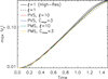Fig. 4. Time evolution of the Kelvin-Helmholtz instability with density contrast of 2. The figure shows the maximum amplitude of the y-component of the velocity without RSST (ξ = 1) in 4096 × 4096 grids (black solid), without RSST (ξ = 1) in the default 1024 × 1024 grids (black dashed), with PVS form (ξ = 10, red), with PVS form (Cmax = 3, blue), with PMS form (ξ = 10, green), and with PMS form (Cmax = 3, yellow).

Figure 5 shows the dependence of the maximum y-component velocity on the reduction parameters (ξ or C_max) of the speed of sound. In the constant ξ cases (panel a), both equations (PVS and PMS forms) show similar ξ-dependence. When the reduction rate is moderate, the result approaches the reference solution because the speed of sound reduction also reduces numerical diffusion. When the reduction rate becomes too large and the effective Mach number approaches unity, the error caused by the RSST increases. Similar parameter dependence also occurs in the constant C_max cases (panel b).

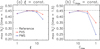Fig. 5. Dependence of the Kelvin-Helmholtz instability with density contrast of 2 on the speed of sound reduction rate with ξ = const. (panel a) and Cmax = const (panel b). In each panel, the maximum amplitude of the y-component of the velocity at time = 1.5 with the PVS form (red with diamond) and the PMS form (blue with cross) are shown. The horizontal dashed line shows the reference simulation results without the RSST (ξ = 1) in 4096 × 4096 grids.

The dependence on the reduction parameters in Fig. 5 can be easily interpreted by using the effective Mach number ξV/a. The dependence on the effective Mach number in Fig. 6 suggests that the effective Mach number should be smaller than 0.3 so that the new RSST methods correctly reproduce the temporal evolution of the Kelvin-Helmholtz instability. We also note that the PVS form performs slightly better than the PMS form in this problem, although the both methods reproduce successful results when the effective Mach number is sufficiently low.

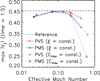Fig. 6. Dependence of the Kelvin-Helmholtz instability with density contrast of 2 on the effective Mach number. The figure shows the maximum amplitude of the y-component of the velocity at time = 1.5 in the PVS form with constant ξ (red solid with diamond), in the PMS form with constant ξ (blue solid with cross), in the PVS form with constant Cmax (red dotted with triangle), and in the PMS form with constant Cmax (blue dotted with box). The horizontal dashed line shows the reference simulation results without the RSST (ξ = 1) in 4096 × 4096 grids.

4.6. Two-dimensional Rayleigh-Taylor instability

We carried out a test problem for the Rayleigh-Taylor instability to clarify the applicability of the proposed methods under the pressure gradient and external forces like gravity. The basic equations are extended to include the effect of gravity F = (0, g_y, 0), as described in Appendix B. The domain size is [0, 1]×[0, 1] in the xy-plane. The boundary condition is periodic in the x-direction. The closed free-slip boundary is used in the y-direction. The initial condition for density is given by

$$\begin{array}{c}\hfill \rho =\{{\rho }_1+\frac{{\rho }_2-{\rho }_1}{2}[1+tan\mathrm{h}\left(\frac{y-1/2}{L}\right)]\}(1+ϵ),\end{array}$$(24)

where ρ₁ = 1.0, ρ₂ = 10.0, and L = 0.025. ϵ is a fraction of the small perturbation on the mass density, which is given by

$$\begin{array}{c}\hfill ϵ=0.01sin\left(4\pi x\right).\end{array}$$(25)

The gas pressure was chosen to achieve hydrostatic balance and is given by

$$\begin{array}{c}\hfill P=P_{\mathrm{c}}-m_{\mathrm{c}}{g}_y,\end{array}$$(26)

where the background column mass density m_c from an arbitrary height y to the top boundary (y = 1) with ϵ = 0 is given by

$$\begin{array}{cc}\hfill m_{\mathrm{c}}& =\frac{1}{2}({\rho }_1+{\rho }_2)(1-y)\hfill \\ \hfill & +\frac{L}{2}({\rho }_2-{\rho }_1)[ln\{exp\left(\frac{1}{2L}\right)+exp(-\frac{1}{2L})\}\hfill \\ \hfill & -ln\{exp\left(\frac{y-1/2}{L}\right)+exp(-\frac{y-1/2}{L})\}],\hfill \end{array}$$(27)

where P_c = 1000 and gravitational acceleration g_y = −1.0. All components of the initial velocity field were zero. The ideal equation of state was used. The specific heat ratio was set to 5/3. Each run was computed with a resolution of 1024 × 1024 grids. The reference solution was simulated in 4096 × 4096 grids without the RSST. A typical Mach number without the RSST is about 0.07 in this problem.

Figure 7 shows the snapshots from the Rayleigh-Taylor instability test problem. The proposed RSST formulations (PVS and PMS forms) reproduce the density pattern, very similar to the reference case. The functional form of the reduction rate (ξ or C_max) does not create any clear discrepancy.

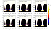Fig. 7. Snapshots from the Rayleigh-Taylor instability at time = 2.5. The color contour shows the mass density without the RSST (ξ = 1; panel a), with PVS form (ξ = 6.3; panel b), with PMS form (ξ = 6.3; panel c), without RSST (ξ = 1) in 4096 × 4096 grids (panel d), with PVS form (Cmax = 10; panel e), and with PMS form (Cmax = 10; panel f). Details of the test problem are discussed in Sect. 4.6.

The applicability of our method to the Rayleigh-Taylor instability can be also confirmed from the time evolution of the maximum amplitude of the y-component of the velocity (Fig. 8). All runs shown in Fig. 7 exhibit very similar time evolution.

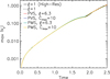Fig. 8. Time evolution of the Rayleigh-Taylor instability. The figure shows the maximum amplitude of the y-component of the velocity without RSST (ξ = 1) in 4096 × 4096 grids (black solid), without RSST (ξ = 1) in the default 1024 × 1024 grids (black dashed), with PVS form (ξ = 6.3, red), with PVS form (Cmax = 10, blue), with PMS form (ξ = 6.3, green), and with PMS form (Cmax = 10, yellow).

The dependence on the speed of sound reduction rate is shown in Fig. 9. As observed in the Kelvin-Helmholtz instability, the proposed method performs well when the reduction rate is not too high. The threshold value of the effective Mach number is again 0.3 (Fig. 10), as was the case in the test problem for the Kelvin-Helmholtz instability.

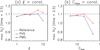Fig. 9. Dependence of the Rayleigh-Taylor instability on the speed of sound reduction rate with ξ = const. (panel a) and Cmax = const (panel b). Each panel shows the maximum amplitude of the y-component of the velocity at time = 2.5 with PVS form (red with diamond) and PMS form (blue with cross). The horizontal dashed line shows the reference simulation results without the RSST (ξ = 1) in 4096 × 4096 grids.

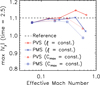Fig. 10. Dependence of the Rayleigh-Taylor instability on the effective Mach number. The maximum amplitude of the y-component of the velocity at time = 2.5 in PVS form with constant ξ (red solid with diamond), in PMS form with constant ξ (blue solid with cross), in PVS form with constant Cmax (red dotted with triangle), and in PMS form with constant Cmax (blue dotted with box). The horizontal dashed line shows the reference simulation results without the RSST (ξ = 1) in 4096 × 4096 grids.

5. Summary and discussion

In this study, we proposed several new formulations of the RSST, which has been applied to accelerate the computational speed in simulations of low Mach number flows. The convergence test of the linear entropy wave and more practical Kelvin-Helmholtz and Rayleigh-Taylor instability problems were carried out. The numerical tests suggest that the effective Mach number (after reducing the speed of sound) should be less than 0.3 in order to maintain the characteristics of the flows. We note that the methods can be easily extended to magnetohydrodynamic equations.

We note that all of new formulations of the RSST are derived by assuming the general equation of state for nonideal gas. Although all of the test problems presented in this paper assume the ideal equation of state. we also carried out several tests using the van der Waals equation of state (e.g., Castro & Toro 2014). Because we could not find any qualitative difference from the ideal equation of state, we believe that our method can work even with a general equation of state.

We summarize the characteristic points of the proposed methods. All of the RSST described in this paper (DVS, DMS, PVS, PMS, and PD) share several characteristics as follows:

• The methods can be easily implemented in an explicit scheme and can accelerate the computational speed of low Mach number flows.

• The steady solution of the RSST equations is the same as the steady solution of the original Euler equations.

• The methods are formulated in semiconservative form so that the equations reduce to the conservative Euler equations when the RSST is not used.

The subgroups of the proposed methods have the following characteristics:

• The newly proposed methods based on the reduction of the temporal evolution of gas pressure (PVS, PMS, and PD forms) share the advantage that the proposed methods can be applied to flows with large density variation.

• The methods based on reduction of density variation (DVS and DMS forms) preserve the modified mass conservation law (∂⟨ξρ⟩/∂t = 0, where ⟨.⟩ indicates a volume average) if the reduction rate is time independent (∂ξ/∂t = 0).

• The DMS and PMS methods employ the exact conservative form of the momentum equations so that the volume integral of the momentum can be conserved down to the round-off error through combination with the finite volume or finite difference methods.

• The PD form is based on the exact conservation laws of both mass and momentum. However, the correct evolution of the entropy can be violated by the pressure variation (see also Appendix A.4).

These various characteristics will broaden the application range of the RSST to a variety of low Mach number phenomena.

Acknowledgments

This work is supported by MEXT/JSPS KAKENHI Grant Number 15H05816. This work was carried out by the joint research program of the Institute for Space-Earth Environment Research (ISEE), Nagoya University. Numerical computations were carried out on a Cray XC50 supercomputer at the Center for Computational Astrophysics, National Astronomical Observatory of Japan.

References

Appendix A: Variants of semiconservative RSST

In this appendix, we describe the original and three alternatives of RSST (DVS, DMS, PMS, and PD forms) in their semiconservative forms. The two new RSST formulations (DMS and PMS forms) are based on the conservative form of the momentum equations rather than the primitive equations of motion, as was the case in the DVS and PVS forms. Accurate conservation of the momentum will be favored in some situations. The PMS form described in Appendix A.2 is based on the reduced pressure evolution. On the other hand, the DMS form described in Appendix A.3 is similar to the DVS form and is derived by reducing the density evolution. The PD form reduces the pressure variation as in the PVS and PMS forms. This new form has the superior conservative property of both mass and momentum in the system, but it does not satisfy the strict form of the entropy equation.

A.1. DVS form for conservative variables

The original DVS form can be rewritten in a semiconservative form given by

$$\begin{array}{cc}& \frac{\partial \rho }{\partial t}+\mathrm{\nabla }·\left(\rho \mathit{V}\right)=-(1-\frac{1}{{\xi }^2})\Delta \rho \hfill \\ \hfill & \frac{\partial }{\partial t}\left(\rho V_i\right)+\mathrm{\nabla }·\left(\rho V_i\mathit{V}\right)+\frac{\partial P}{\partial x_i}=-(1-\frac{1}{{\xi }^2}){\left(\frac{\partial \rho V_i}{\partial \rho }\right)}_{\mathit{V}}\Delta \rho \hfill \\ \hfill & \frac{\partial E}{\partial t}+\mathrm{\nabla }·\left[(E+P)\mathit{V}\right]=-(1-\frac{1}{{\xi }^2}){\left(\frac{\partial E}{\partial \rho }\right)}_{\mathit{V},S}\Delta \rho ,\hfill \end{array}$$(A.1)

where

$$\begin{array}{c}\hfill \Delta \rho =-\mathrm{\nabla }·\left(\rho \mathit{V}\right)\end{array}$$(A.2)

is the time variation of the mass density without the RSST and

$$\begin{array}{c}\hfill {\left(\frac{\partial \rho V_i}{\partial \rho }\right)}_{\mathit{V}}=V_i,{\left(\frac{\partial E}{\partial \rho }\right)}_{\mathit{V},S}=\frac{e+P+\rho V^2/2}{\rho }·\end{array}$$(A.3)

As shown in Sect. 4, the DVS form in this semiconservative formulation also has a drawback in that it is not applicable to flows with large density variation.

A.2. Momentum conservative form based on pressure variation reduction (PMS form)

The PMS form is an alternative of the PVS form (Sect. 3) that strictly conserves the momentum of the system if the momentum flux through the boundary is negligible. The basic equations of the PMS form are the evolution equations of (P, ρV, S), which are given by

$$\begin{array}{cc}& {\xi }^2\frac{\partial P}{\partial t}+\mathit{V}·\mathrm{\nabla }P+\rho a^2\mathrm{\nabla }·\mathit{V}=0\hfill \\ \hfill & \frac{\partial }{\partial t}\left(\rho V_i\right)+\mathrm{\nabla }·\left(\rho V_i\mathit{V}\right)+\frac{\partial P}{\partial x_i}=0\hfill \\ \hfill & \frac{\partial S}{\partial t}+\mathit{V}·\mathrm{\nabla }S=0.\hfill \end{array}$$(A.4)

The only difference from the PVS form is the use of the conservative form of the momentum equations instead of the primitive equations of motion. Apparently, this formulation conserves the volume average of the momentum in the isolated system.

The phase speeds of each wave mode in Eq. (A.4) are different from those in the DVS or PVS forms. From the one-dimensional version of Eq. (A.4),

$$\frac{\partial }{\partial t}\left(\begin{array}{c}P\\ \rho V_x\\ S\end{array}\right)+A\frac{\partial }{\partial x}\left(\begin{array}{c}P\\ \rho V_x\\ S\end{array}\right)=0,$$(A.5)

$$A=\left(\begin{array}{ccc}0& a^2/{\xi }^2& P_S{V}_x/{\xi }^2\\ 1-V_x^2/a^2& 2V_x& P_S{V}_x^2/a^2\\ 0& 0& V_x\end{array}\right),$$(A.6)

and the wave speeds are given by

$$\begin{array}{c}\hfill \lambda =\{\begin{array}{c}{V}_x,\hfill \\ V_x\pm \sqrt{D}\hfill \end{array}\mathrm{where}D=(1-\frac{1}{{\xi }^2})V_x^2+\frac{1}{{\xi }^2}{a}^2.\end{array}$$(A.7)

Because ξ ≥ 1 is always satisfied in order to limit the speed of sound, all wave speeds are real (D >  0) and Eq. (A.4) are hyperbolic. The effective speed of sound $\sqrt{D}$ is larger than the absolute value of the velocity |V_x| and is smaller than the real speed of sound a. In the low Mach number limit (|V_x|≪a), the effective speed of sound $\sqrt{D}$ approaches a/ξ as was the case in the original RSST. Thus, this new formulation can be used to reduce the speed of sound in low Mach number flows.

The momentum conserving PMS form can be also rewritten as evolution equations in terms of the conservative variables. The semiconservative form of Eq. (A.4) is given by

$$\begin{array}{cc}& \frac{\partial \rho }{\partial t}+\mathrm{\nabla }·\left(\rho \mathit{V}\right)=-(1-\frac{1}{{\xi }^2}){\left(\frac{\partial \rho }{\partial P}\right)}_S\Delta P\hfill \\ \hfill & \frac{\partial }{\partial t}\left(\rho V_i\right)+\mathrm{\nabla }·\left(\rho V_i\mathit{V}\right)+\frac{\partial P}{\partial x_i}=0\hfill \\ \hfill & \frac{\partial E}{\partial t}+\mathrm{\nabla }·\left[(E+P)\mathit{V}\right]=-(1-\frac{1}{{\xi }^2}){\left(\frac{\partial E}{\partial P}\right)}_{\rho \mathit{V},S}\Delta P,\hfill \end{array}$$(A.8)

where ΔP has the same definition in Eq. (17) and

$$\begin{array}{c}\hfill {\left(\frac{\partial E}{\partial P}\right)}_{\rho \mathit{V},S}=\frac{e+P-\rho V^2/2}{\rho a^2}·\end{array}$$(A.9)

Apparently, the momentum equations are in a complete conservative form.

As tested in Sect. 4, we cannot find any significant drawback that arises from using the conservative form in the momentum equations. For application to problems where (angular) momentum conservation is important, the PMS form will have some advantages.

A.3. Momentum conservative form based on density variation reduction (DMS form)

The DMS form is based on reducing the density variation, similar to the DVS form (Sect. 2 and Appendix A.1). The difference is that the DMS form employs the conservative form of the momentum equations. The basic equations of the DMS form are the evolution equations of (ρ, ρV, S), which are given by

$$\begin{array}{cc}& {\xi }^2\frac{\partial \rho }{\partial t}+\mathrm{\nabla }·\left(\rho \mathit{V}\right)=0\hfill \\ \hfill & \frac{\partial }{\partial t}\left(\rho V_i\right)+\mathrm{\nabla }·\left(\rho V_i\mathit{V}\right)+\frac{\partial P}{\partial x_i}=0\hfill \\ \hfill & \frac{\partial S}{\partial t}+\mathit{V}·\mathrm{\nabla }S=0.\hfill \end{array}$$(A.10)

The wave speed is same as the PMS form and is given in Eq. (A.7).

The semiconservative version of the DMS form is given by

$$\begin{array}{cc}& \frac{\partial \rho }{\partial t}+\mathrm{\nabla }·\left(\rho \mathit{V}\right)=-(1-\frac{1}{{\xi }^2})\Delta \rho \hfill \\ \hfill & \frac{\partial }{\partial t}\left(\rho V_i\right)+\mathrm{\nabla }·\left(\rho V_i\mathit{V}\right)+\frac{\partial P}{\partial x_i}=0\hfill \\ \hfill & \frac{\partial E}{\partial t}+\mathrm{\nabla }·\left[(E+P)\mathit{V}\right]=-(1-\frac{1}{{\xi }^2}){\left(\frac{\partial E}{\partial \rho }\right)}_{\rho \mathit{V},S}\Delta \rho ,\hfill \end{array}$$(A.11)

where Δρ has the same definition in Eq. (17) and

$$\begin{array}{c}\hfill {\left(\frac{\partial E}{\partial \rho }\right)}_{\rho \mathit{V},S}=\frac{e+P-\rho V^2/2}{\rho }·\end{array}$$(A.12)

Because the drawback of the DVS form described in Sect. 2.2 is independent from the form of the momentum equations in the basic equations, the DMS form has the same drawback as was the case in the DVS form.

A.4. Mass and momentum conservative form based on pressure variation reduction (PD form)

We can also construct a form of the RSST that strictly conserves both mass and momentum in the closed system. The PD form is based on the pressure variation reduction method as follows:

$$\begin{array}{cc}& {\xi }^2\frac{\partial P}{\partial t}+\mathit{V}·\mathrm{\nabla }P+\rho a^2\mathrm{\nabla }·\mathit{V}=0\hfill \\ \hfill & \frac{\partial V_i}{\partial t}+\mathit{V}·\mathrm{\nabla }{V}_i+\frac{1}{\rho }\frac{\partial P}{\partial x_i}=0\hfill \\ \hfill & \frac{\partial \rho }{\partial t}+\mathrm{\nabla }·\left(\rho \mathit{V}\right)=0.\hfill \end{array}$$(A.13)

The wave speeds λ of Eq. (A.13) are identical to the speeds in DVS and PVS forms and given by Eqs. (6) and (7).

The semiconservative equations of the PD form is given by

$$\begin{array}{cc}& \frac{\partial \rho }{\partial t}+\mathrm{\nabla }·\left(\rho \mathit{V}\right)=0\hfill \\ \hfill & \frac{\partial }{\partial t}\left(\rho V_i\right)+\mathrm{\nabla }·\left(\rho V_i\mathit{V}\right)+\frac{\partial P}{\partial x_i}=0\hfill \\ \hfill & \frac{\partial E}{\partial t}+\mathrm{\nabla }·\left[(E+P)\mathit{V}\right]=-(1-\frac{1}{{\xi }^2}){\left(\frac{\partial E}{\partial P}\right)}_{\mathit{V},\rho }\Delta P,\hfill \end{array}$$(A.14)

where

$$\begin{array}{c}\hfill {\left(\frac{\partial E}{\partial P}\right)}_{\mathit{V},\rho }={\left(\frac{\partial e}{\partial P}\right)}_{\rho },\end{array}$$(A.15)

and the ΔP is defined by Eq. (17). Apparently, the PD form employs the exact form of the mass and momentum conservation laws. This characteristic is advantageous when both mass and momentum conservation are important.

Although the PD form has the superior conservative property of the mass and momentum, the user should be careful when this form is applied to practical problems. From Eq. (A.13), the entropy equation in the PD form is given by

$$\begin{array}{c}\hfill P_S\frac{\mathit{DS}}{\mathit{Dt}}=(1-\frac{1}{{\xi }^2})\Delta P,\end{array}$$(A.16)

where P_S = (∂P/∂S)_ρ as described in Sect. 2.1. Equation (A.16) indicates that the pressure variation (e.g., sound wave) can change the specific entropy artificially. Although the PD form performs well in all of the test problems described in this paper, such violation of the entropy evolution can be a possible source of error in more severe problems. One example is the thermal convection in the deep stellar convection zone where the very small variation of the entropy drives the convective motion through the buoyancy force (i.e., the super-adiabaticity is very small), although the convective motion continuously excites sound waves.

Appendix B: Extension of the RSST with an external force

We need to include the effect of an external force (gravity) for simulation of the two-dimensional Rayleigh-Taylor instability in Sect. 4.6.

The basic equations of the PVS form are extended to the case with an external force F as follows: (1) We add ρF and ρV ⋅ F to the right-hand side of the momentum and total energy equations of Eq. (15) or Eq. (19), respectively. (2) The definition of ΔP in Eq. (17) or Eq. (21) remains unchanged. The resulting equations are given by

$$\begin{array}{cc}& \frac{\partial \rho }{\partial t}+\mathrm{\nabla }·\left(\rho \mathit{V}\right)=-(1-\frac{1}{{\xi }^2}){\left(\frac{\partial \rho }{\partial P}\right)}_S\Delta P\hfill \\ \hfill & \frac{\partial }{\partial t}\left(\rho V_i\right)+\mathrm{\nabla }·\left(\rho V_i\mathit{V}\right)+\frac{\partial P}{\partial x_i}=-(1-\frac{1}{{\xi }^2}){\left(\frac{\partial \rho V_i}{\partial P}\right)}_{\mathit{V},S}\Delta P+\rho \mathit{F}\hfill \\ \hfill & \frac{\partial E}{\partial t}+\mathrm{\nabla }·\left[(E+P)\mathit{V}\right]=-(1-\frac{1}{{\xi }^2}){\left(\frac{\partial E}{\partial P}\right)}_{\mathit{V},S}\Delta P+\rho \mathit{V}·\mathit{F},\hfill \end{array}$$(B.1)

where ΔP and the partial derivatives (∂ρ/∂P)_S, (∂ρV_i/∂P)_V,S, and (∂E/∂P)_V,S are given in Eqs. (17) and (16), respectively.

The PMS, DVS, DMS, and PD forms can be extended in a similar fashion.

All Figures

Fig. 1. Convergence test of linear entropy wave. The horizontal axis N represents the number of grid points used in the x-direction. Shown are the L1 errors of the specific entropy (panel a), velocity component normal to the propagation direction of wave V⊥ (panel b), mass density (panel c), and gas pressure (panel d). Each line corresponds to the form of RSST used in the simulation. The dashed line in each panel shows the analytical line of second-order convergence. Details of the test problem are given in Sect. 4.4.

In the text

Fig. 2. Snapshots from the Kelvin-Helmholtz instability with low density contrast at time = 1.5. The normalized density variation Δρ/Δρ0 = (ρ − ρ1)/(ρ2 − ρ1) is shown. Top row: results with density contrast of 1.5. Bottom row: results with density contrast of 1.001. Each column corresponds to a different reduction method for the speed of sound: without the RSST (ξ = 1; panels a and d), with the PVS form (ξ = 3; panels b and e), and with the DVS form (ξ = 3; panels c and f). Details of the test problem are given in Sect. 4.5.

In the text

Fig. 3. Snapshots of the Kelvin-Helmholtz instability with density contrast of 2 at time = 1.5. The color contour shows the mass density without the RSST (ξ = 1; panel a), with the PVS form (ξ = 10; panel b), with the PMS form (ξ = 10; panel c), without the RSST (ξ = 1) in 4096 × 4096 grids (panel d), with the PVS form (Cmax = 3; panel e), and with the PMS form (Cmax = 3; panel f). The detail of the test problem is shown in Sect. 4.5.

In the text

Fig. 4. Time evolution of the Kelvin-Helmholtz instability with density contrast of 2. The figure shows the maximum amplitude of the y-component of the velocity without RSST (ξ = 1) in 4096 × 4096 grids (black solid), without RSST (ξ = 1) in the default 1024 × 1024 grids (black dashed), with PVS form (ξ = 10, red), with PVS form (Cmax = 3, blue), with PMS form (ξ = 10, green), and with PMS form (Cmax = 3, yellow).

In the text

Fig. 5. Dependence of the Kelvin-Helmholtz instability with density contrast of 2 on the speed of sound reduction rate with ξ = const. (panel a) and Cmax = const (panel b). In each panel, the maximum amplitude of the y-component of the velocity at time = 1.5 with the PVS form (red with diamond) and the PMS form (blue with cross) are shown. The horizontal dashed line shows the reference simulation results without the RSST (ξ = 1) in 4096 × 4096 grids.

In the text

Fig. 6. Dependence of the Kelvin-Helmholtz instability with density contrast of 2 on the effective Mach number. The figure shows the maximum amplitude of the y-component of the velocity at time = 1.5 in the PVS form with constant ξ (red solid with diamond), in the PMS form with constant ξ (blue solid with cross), in the PVS form with constant Cmax (red dotted with triangle), and in the PMS form with constant Cmax (blue dotted with box). The horizontal dashed line shows the reference simulation results without the RSST (ξ = 1) in 4096 × 4096 grids.

In the text

	Fig. 7. Snapshots from the Rayleigh-Taylor instability at time = 2.5. The color contour shows the mass density without the RSST (ξ = 1; panel a), with PVS form (ξ = 6.3; panel b), with PMS form (ξ = 6.3; panel c), without RSST (ξ = 1) in 4096 × 4096 grids (panel d), with PVS form (Cmax = 10; panel e), and with PMS form (Cmax = 10; panel f). Details of the test problem are discussed in Sect. 4.6.
In the text

	Fig. 8. Time evolution of the Rayleigh-Taylor instability. The figure shows the maximum amplitude of the y-component of the velocity without RSST (ξ = 1) in 4096 × 4096 grids (black solid), without RSST (ξ = 1) in the default 1024 × 1024 grids (black dashed), with PVS form (ξ = 6.3, red), with PVS form (Cmax = 10, blue), with PMS form (ξ = 6.3, green), and with PMS form (Cmax = 10, yellow).
In the text

Fig. 9. Dependence of the Rayleigh-Taylor instability on the speed of sound reduction rate with ξ = const. (panel a) and Cmax = const (panel b). Each panel shows the maximum amplitude of the y-component of the velocity at time = 2.5 with PVS form (red with diamond) and PMS form (blue with cross). The horizontal dashed line shows the reference simulation results without the RSST (ξ = 1) in 4096 × 4096 grids.

In the text

Fig. 10. Dependence of the Rayleigh-Taylor instability on the effective Mach number. The maximum amplitude of the y-component of the velocity at time = 2.5 in PVS form with constant ξ (red solid with diamond), in PMS form with constant ξ (blue solid with cross), in PVS form with constant Cmax (red dotted with triangle), and in PMS form with constant Cmax (blue dotted with box). The horizontal dashed line shows the reference simulation results without the RSST (ξ = 1) in 4096 × 4096 grids.

In the text

References

- Cai, T. 2016, J. Comput. Phys., 310, 342 [NASA ADS] [CrossRef] [Google Scholar]
- Castro, C. E., & Toro, E. F. 2014, Int. J. Numer. Methods Fluids, 75, 467 [NASA ADS] [CrossRef] [Google Scholar]
- Chan, K. L., Mayr, H. G., Mengel, J. G., & Harris, I. 1994, J. Comput. Phys., 113, 165 [NASA ADS] [CrossRef] [Google Scholar]
- Dumbser, M., & Balsara, D. S. 2016, J. Comput. Phys., 304, 275 [NASA ADS] [CrossRef] [Google Scholar]
- Dumbser, M., & Toro, E. F. 2011, J. Sci. Comput., 48, 70 [Google Scholar]
- Gardiner, T. A., & Stone, J. M. 2005, J. Comput. Phys., 205, 509 [Google Scholar]
- Glasner, S. A., Livne, E., & Truran, J. W. 2007, ApJ, 665, 1321 [NASA ADS] [CrossRef] [Google Scholar]
- Gottlieb, S., Ketcheson, D. I., & Shu, C.-W. 2009, J. Sci. Comput., 38, 251 [Google Scholar]
- Hotta, H., Rempel, M., & Yokoyama, T. 2014, ApJ, 786, 24 [NASA ADS] [CrossRef] [Google Scholar]
- Hotta, H., Rempel, M., & Yokoyama, T. 2015, ApJ, 798, 51 [NASA ADS] [CrossRef] [Google Scholar]
- Hotta, H., Rempel, M., Yokoyama, T., Iida, Y., & Fan, Y. 2012, A&A, 539, A30 [NASA ADS] [CrossRef] [EDP Sciences] [Google Scholar]
- Hotta, H., Rempel, M., & Yokoyama, T. 2016, Science, 351, 1427 [NASA ADS] [CrossRef] [Google Scholar]
- Hou, T. Y., & Lefloch, P. G. 1994, Math. Comput., 62, 497 [NASA ADS] [CrossRef] [MathSciNet] [Google Scholar]
- Iijima, H., & Yokoyama, T. 2015, ApJ, 812, L30 [NASA ADS] [CrossRef] [Google Scholar]
- Iijima, H., & Yokoyama, T. 2017, ApJ, 848, 38 [NASA ADS] [CrossRef] [Google Scholar]
- Käpylä, P. J., Brandenburg, A., Kleeorin, N., Käpylä, M. J., & Rogachevskii, I. 2016, A&A, 588, A150 [NASA ADS] [CrossRef] [EDP Sciences] [Google Scholar]
- Kupka, F., & Muthsam, H. J. 2017, Living Rev. Comput. Astrophys., 3, 1 [NASA ADS] [CrossRef] [Google Scholar]
- McNally, C. P., Lyra, W., & Passy, J.-C. 2012, ApJS, 201, 18 [NASA ADS] [CrossRef] [Google Scholar]
- Miesch, M. S., Brun, A. S., De Rosa, M. L., & Toomre, J. 2008, ApJ, 673, 557 [NASA ADS] [CrossRef] [Google Scholar]
- Nonaka, A., Almgren, A. S., Bell, J. B., et al. 2010, ApJS, 188, 358 [NASA ADS] [CrossRef] [Google Scholar]
- Nordlund, Å. 1982, A&A, 107, 1 [Google Scholar]
- Rempel, M. 2005, ApJ, 622, 1320 [NASA ADS] [CrossRef] [Google Scholar]
- Rempel, M., Schüssler, M., & Knölker, M. 2009, ApJ, 691, 640 [NASA ADS] [CrossRef] [Google Scholar]
- Stein, R. F., & Nordlund, Å. 1989, ApJ, 342, L95 [NASA ADS] [CrossRef] [PubMed] [Google Scholar]
- Takeyama, K., Saitoh, T. R., & Makino, J. 2017, New A, 50, 82 [NASA ADS] [CrossRef] [Google Scholar]
- van Leer, B. 1979, J. Comput. Phys., 32, 101 [Google Scholar]
- Vögler, A., Shelyag, S., Schüssler, M., et al. 2005, A&A, 429, 335 [NASA ADS] [CrossRef] [EDP Sciences] [Google Scholar]
- Zingale, M., Woosley, S. E., Rendleman, C. A., Day, M. S., & Bell, J. B. 2005, ApJ, 632, 1021 [NASA ADS] [CrossRef] [Google Scholar]