| Issue |
A&A
Volume 621, January 2019
|
|
|---|---|---|
| Article Number | A127 | |
| Number of page(s) | 13 | |
| Section | Interstellar and circumstellar matter | |
| DOI | https://doi.org/10.1051/0004-6361/201834405 | |
| Published online | 17 January 2019 | |
Low-frequency measurements of synchrotron absorbing HII regions and modeling of observed synchrotron emissivity
1
Department of Astrophysics/IMAPP, Radboud University,
PO Box 9010,
6500
GL Nijmegen,
The Netherlands
e-mail: i.polderman@astro.ru.nl
2
CRESST II, NASA Goddard Space Flight Center, Greenbelt,
MD,
20771,
USA
3
Department of Astronomy, University of Maryland,
College Park,
MD,
20742,
USA
Received:
8
October
2018
Accepted:
24
November
2018
Context. Cosmic rays (CRs) and magnetic fields are dynamically important components in the Galaxy, and their energy densities are comparable to that of the turbulent interstellar gas. The interaction of CRs and Galactic magnetic fields (GMF) produces synchrotron radiation clearly visible in the radio regime. Detailed measurements of synchrotron radiation averaged over the line-of-sight (LOS), so-called synchrotron emissivities, can be used as a tracer of the CR density and GMF strength.
Aims. Our aim is to model the synchrotron emissivity in the Milky Way using a three-dimensional dataset instead of LOS-integrated intensity maps on the sky.
Methods. Using absorbed HII regions, we measured the synchrotron emissivity over a part of the LOS through the Galaxy, changing from a two-dimensional to a three-dimensional view. Performing these measurements on a large scale is one of the new applications of the window opened by current low-frequency arrays. Using various simple axisymmetric emissivity models and a number of GMF-based emissivity models, we were able to simulate the synchrotron emissivities and compare them to the observed values in the catalog.
Results. We present a catalog of low-frequency absorption measurements of HII regions, their distances and electron temperatures, compiled from literature. These data show that the axisymmetric emissivity models are not complex enough, but the GMF-based emissivity models deliver a reasonable fit. These models suggest that the fit can be improved by either an enhanced synchrotron emissivity in the outer reaches of the Milky Way or an emissivity drop near the Galactic center.
Conclusions. Current GMF models plus a constant CR density model cannot explain low-frequency absorption measurements, but the fits improved with slight (ad hoc) adaptations. It is clear that more detailed models are needed, but the current results are very promising.
Key words: cosmic rays / ISM: magnetic fields / HII regions / Galaxy: structure / radio continuum: ISM / catalogs
© ESO 2019
1 Introduction
Cosmic rays (CRs) play an important role in many aspects of Galaxy ecology (Grenier et al. 2015). Consequently, understanding more about these particles is a big leap forward in understanding our own Galaxy. In general, CRs moderate processes by depositing or taking away energy. For example, the CRs that are accelerated in a supernova remnant (SNR) take away between 10% and 50% of the SNR energy. This lowers the temperature of the remnant and changes the impact of the SNR on the interstellar medium (ISM). The presence of relativistic particles also causes a longer expansion time for the SNR, thereby increasing the momentum that can be deposited in the ISM (Diesing & Caprioli 2018). While CRs diffuse through the Galaxy, their interactions with the ISM cause them to deposit energy along kiloparsecs. The interactions can cause ionization and heating of dense interstellar gas, thereby keeping the darkest ISM at temperatures near 10 K, for example. This also makes CRs very important for driving chemistry at low temperatures. CRs are also thought to drive magnetohydrodynamic waves, which could maintain interstellar turbulence, and largescale interstellar flows. Among these flows are Galactic winds, fountains and possibly bubbles – like the Fermi bubbles, (e.g., Su et al. 2010; Mertsch & Petrosian 2017). Furthermore, CRs probe objects and environments in the Galaxy, like stellar atmospheres, the composition of accelerated matter, and the total gas content of interstellar clouds. CRs also interact with the Galactic magnetic field (GMF). This interaction produces the synchrotron radiation that dominates the radio spectrum at low radio frequencies. At these frequencies, the synchrotron intensity can be used as a measure for both the CR number density, nCR, and the strength of the magnetic field, B⊥, perpendicular to the line-of-sight (LOS; Webber 1977; Jaffe et al. 2010)
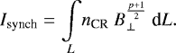 (1)
(1)
The value of p in the exponent of the magnetic field is assumed to be 3, which follows from the CR spectrum, (Planck Collaboration XXV 2016).
One complication of this tracer is however, the averaging over the entire LOS. It is unlikely that the synchrotron emission is constant along the LOS. To partially overcome this issue, the low-frequency regime opens up the possibility to integrate over only part of it. To accomplish this, observations of HII regions with known distances are used, essentially elevating this kind of work from a two-dimensional view (total LOS) of Galactic synchrotron emission to a three-dimensional one (partial LOS).
Scheuer & Ryle (1953) were among the first to consider the HII region effect on synchrotron, or non-thermal, radiation. And Shain (1959) showed that at low frequencies free–free absorption starts to play an important role. This absorption is characteristic for an optically thick HII region, where the free–free opacity, τ > 1, which is only the case at lower frequencies (ν ≲ 150 MHz, Hindson et al. 2016). Several papers are dedicated to determining the spectral turnover frequency for the free–free emission of Galactic HII regions (e.g., Mezger & Henderson 1967; Hindson et al. 2016), below which the opacity increases and HII regions are observed as absorption regions against a Galactic synchrotron background emission. As we explain in detail in Sect. 2, using low-frequency observations of HII regions allows one to integrate over only a section of the LOS. Several papers (e.g., Jones & Finlay 1974; Caswell 1976; Roger et al. 1999; Nord et al. 2006; Hindson et al. 2016; Su et al. 2016) determine synchrotron emissivity values using this method. These observations can be used to gain insight into CR density and magnetic field strength in the Milky Way, and different models can be used to describe the observed values (Nord et al. 2006; Su et al. 2016). In this paper these models are known as the simple axisymmetric emissivity models.
Another complication of using synchrotron as a tracer is the fact that it is a convolved effect of both the CR density and the magnetic field strength. It is clear that CR particles are strongly coupled to magnetic fields, and a commonly used simplification is the assumption of equipartition (e.g., Beck 2015; Ferrière 2016) between the energy densities of the CRs and the magnetic field. This assumption is plausible on large scales, but less likely on scales of (tens of) parsecs. If we want to draw any conclusions about CR density and GMF strength in the Milky Way, we will need an assumption like equipartition. In this work we also try another approach, by using existing GMF models and an assumed CR density model to compute synchrotron emissivity. In this paper the combined GMF and CR density models, are known as the GMF-based emissivity models. The variations in the emission are based solely on the (different) details in the GMF models. By comparing the simulated and observed emission, we can begin to understand the differences between them and between the GMF models.
This paper is constructed as follows. In Sect. 2 we discuss Galactic absorption features and extracting synchrotron emissivity. In Sect. 3 we discuss the data we have collected from HII region observations, and in Sect. 4 we describe the effort of combining these data into one coherent master catalog. In Sect. 5 we discuss the features in the observed emissivities. Section 6 describes the modeling effort and its results are discussed in Sect. 7. Section 8 contains the discussion of this work and Sect. 9 gives our conclusions. In Sect. 10 we discuss future work.
2 Galactic absorption features and synchrotron emissivity
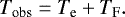
We explain the interpretation of measurements of Galactic free–free absorption. For low radio frequency observationsof HII regions, with an absolute calibration of the flux, the observed brightness temperature Tobs is (Kassim 1990)
 (2)
(2)
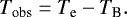
where TF is the brightness temperature of the synchrotron emission between the observer and the HII region (foreground) and TB is the brightness temperatureof the synchrotron emission behind the HII region (background). The HII region is described by the electron temperature, Te, and τ, the opacity. When observing at low frequencies, τ ≫ 1, so the equation reduces to
 (3)
(3)
For observations without absolute calibration (usually the case for interferometric data), the large-scale flux is unobserved, which can be envisioned as subtracting the total temperature TT = TF + TB to obtain

Using the high-opacity approximation for the low frequencies, we get
 (6)
(6)
At low frequencies TB > Te is generally valid, so that Tobs < 0. The electron temperature can be estimated or it can be derived from higher frequency observations (e.g. Paladini et al. 2004; Alves et al. 2012; Balser et al. 2015).
Depending on the type of measurement (single dish or interferometer) and the calibration (absolute or not), we obtain the emissivity ϵ in either the foreground or the background of an HII region as

where DF is the distance to the HII region and DB is the distance from the HII region to the edge of the synchrotron disk, along the LOS. For both of these distances, we use the term path length. We assumed a Galactic disk with a radius of 20 kpc and a solar distance to the Galactic center of 8.5 kpc. Usually HII region distances are determined kinematically, for nearby HII regions it can be done by determining the spectral type of the ionizing star. Another method uses the association with a maser with a measured parallax (Anderson et al. 2014).
The correct foreground and background temperatures can only be achieved if the opacity τ ≫ 1 across the observing beam. Therefore, we have considered only HII regions that are larger than the beam.
3 Data
We used data from five published papers to build our catalog. Relevant details of these papers are presented in Table 1. We refer to these papers by the number assigned to them in Table 1.
3.1 Background on papers used
Jones & Finlay (1974), hereafter Paper 1, mapped brightness temperatures near the Galactic plane between Galactic longitudes ℓ = 225° and ℓ = 30° from a survey with the telescope in Fleurs, N.S.W. (Finlay & Jones 1973) at 29.9 MHz. These authors observed 29 absorption features of which two are optically thick across the beam. The absolute calibration for this data, by using a 30 MHz Parkes survey (Mathewson et al. 1965) among others, results in foreground synchrotron emissivities for the HII regions from this paper.
Roger et al. (1999), hereafter Paper 2, used data taken with the 22 MHz telescope at the Dominion Radio Astrophysical Observatory (DRAO), in Penticton B.C. Canada (Costain et al. 1969), in the period between 1965 and 1969. They mapped the 22 MHz emission between ℓ = − 28° and ℓ = +80°. These observations include 21 HII regions of which eight were larger than the beam. We discard G6.3+26.5 because of its high latitude, its location in the direction of the North Polar Spur and its anomalously high observed emissivity. These authors performed an absolute calibration of their data by considering the average brightness temperature ratio between their data and data from the absolute calibrated 408 MHz all-sky survey by Haslam et al. (1982). Their contribution to this catalog consists of foreground emissivities only.
Nord et al. (2006), hereafter Paper 3, observe four fields along the Galactic plane between ℓ = 349° and ℓ = 21.5° with the VLA in compact configuration at 74 MHz. Their goal was a dedicated search for absorption features in the Galactic plane. The observations include 92 HII regions of which 41 had known distances and thus, are usable. To identify HII regions, Paper 3 used an a priori search for HII absorption features, at locations of known HII regions from Paladini et al. (2003). This paper has done no absolute calibration, therefore the emissivities obtained are background emissivities.
Hindson et al. (2016), hereafter Paper 4, use data taken as part of the Galactic and Extragalactic All-sky MWA survey, (GLEAM; Hurley-Walker et al. 2017). This survey uses multiple frequency bands between 72 and 231 MHz. The authors of Paper 4 make use of this wide frequency range to identify the characteristic spectrum generated by the thermal Brehmsstrahlung process in HII regions. Largescale background emission observed by MWA is subtracted so that Eq. (6) holds. Out of the 302 detected HII regions 29 have known distances. A further two are discarded because they are smaller than the beam.
Su et al. (2016), hereafter Paper 5 use part of the data from the GLEAM survey at 88 MHz, between ℓ = 250° and ℓ = 355°, to measure free–free absorption of the Galactic synchrotron emission by intervening HII regions along the LOS. They perform a dedicated search for absorption regions, at locations of known HII regions from Anderson et al. (2014), and find 47 that are usable. Like Paper 4, they subtract the large-scale background emission.
Source paper observing parameters.
3.2 Flux calibration
Since some of the data used are over 50 years old, we checked that all data are calibrated to the same standardized flux levels. Paper 1 uses Hydra A – also known as 3C218 – as a calibrator, with a flux at 29.9 MHz measured as 1512 ± 81 Jy (Finlay & Jones 1973). Both Papers 2 and 3 use Cygnus A as a calibrator. Paper 2 uses a flux for Cygnus A of 29100 ± 1500 Jy at 22 MHz (Roger 1969). Paper 3 uses the Baars et al. (1977) flux scale of 1706 ± 50 Jy at 74 MHz, which also states a value of 29100 ± 1750 Jy at 22 MHz. These two values for the flux of Cygnus A are consistent. The flux of Hydra A according to the Baars et al. (1977) flux scaling would be 1426 ± 89 Jy at 29.9 MHz, in agreement with the values found in Finlay & Jones (1973). Both Papers 4 and 5 used the GLEAM survey (Hurley-Walker et al. 2017) to find their HII regions. This survey has calibrated all their data with the flux scales found in Baars et al. (1977). We conclude that the different flux scalings for calibrators used in the various papers are consistent, therefore no scaling is needed.
Source paper catalog contributions.
4 Building a low-frequency catalog
In this chapter we discuss what computations have been done with the data from Papers 1–5 to compile them into one coherent low-frequency catalog, rescaled to 74 MHz. The complete low-frequency catalog can be found at the end of this paper, in Table A.1. A graphic representation of all line-of-sight in the catalog can be found in Fig. 9.
4.1 Additions and updates to published data
4.1.1 Brightness temperatures
Paper 1 did not published errors on the observed brightness temperature, Tmin in their Table 2. In their discussion they conclude that the absolute calibration introduces an uncertainty of roughly 2000 K, which is one part of the total error. The second part is based on the root mean square noise level based on the aerial temperatures and is thought to be ~ 900–4400 K depending on the location on the sky. The weighted mean of these errors is calculated for both HII regions.
We use the electron and foreground temperatures to calculate a brightness temperature for the HII regions in Paper 2. Because of an incomplete discussion on the uncertainties for their measurements we choose to use an error of 104 K on each brightness temperature. This error translates to roughly an 18–40% uncertainty of the observed temperatures. This spread is similar to the one in the uncertainties for the rest of the observed temperatures in the catalog.
Published data in Paper 4 consist of integrated surface brightnesses in Jy. To compare these to the rest of the catalog data, a mean surface brightness per beam was calculated for each HII region. We did this by using the size of the HII region and calculating the number of beams covering the HII region, which gives the surface brightness in Jy beam−1. Using the Rayleigh–Jeans law, we calculated the brightness temperature at 88 MHz before rescaling to 74 MHz.
4.1.2 Distances
The distance errors in Paper 1 were found in Georgelin & Georgelin (1970), one of multiple papers mentioned by the authors. Paper 2 provided their distances without any uncertainties, which can be found in Georgelin & Georgelin (1970) and Humphreys (1978). From these papers we have been able to reconstruct the error for each HII region distance, except for one, for which we have assumed an uncertainty of roughly 10% of the distance. The mean relative distance uncertainty in the HII region sample for this is 15%. Paper 3 provides distances without uncertainties, but they reference Paladini et al. (2003) for their HII region distances. We used the radial velocities from this referenced paper, together with their discussion on kinematic distances, to calculate the proper distance errors and to check all the values in the catalog entries for Paper 3. For one HII region the quoted distance was different from our own investigation and we have replaced their value with our new one.
4.1.3 Electron temperatures and the electron temperature gradient with Galactocentric radius
For 59 HII regions out of our current sample of 124, the electron temperatures have been determined through measurements of hydrogen radio recombination lines and continuum. However, for the other 65 HII regions, no measurements were available and various values for their electron temperature have been adopted: Te =104 K in Paper 4, Te =7000 K in Paper 3, or following the gradient with Galactocentric radius as given by Balser et al. (2015) in Paper 5. We investigated whether the assumed values for Te need to be adapted for consistency, in our catalog. Various values of electron temperature gradients have been published (e.g., Paladini et al. 2004; Alves et al. 2012; Balser et al. 2015), which are not always in agreement with each other. However, Balser et al. (2015) conclude that there is also azimuthal variation of electron temperatures of HII regions in the Milky Way. Therefore, gradients of electron temperature with Galactocentric radius are expected to vary for different spatial distributions of used sources. Due to the absence of well-defined electron temperatures in Paper 1, we decided to update these for the HII regions in this set. We have used values from a more recent survey by Azcárate et al. (1990). Paper 2 does not discuss the origin or uncertainty of their electron temperature of 6000 K; based on the electron temperaturevalues for the other catalog entries, we have assumed an uncertainty of 1000 K. For a sample of 19 HII regions, Paper 4 does not provide electron temperatures. We have assumed an electron temperature of 7000 K ± 2000 K. All measured and assumed electron temperatures in our catalog are plotted in Fig. 1. This figure shows that the assumed values for electron temperatures are in the same temperature range as the measured temperatures. Furthermore, there is such a large variation in measured temperature between individual HII regions that we do not think that adapting the assumed temperatures to any of the published gradients is useful. Hence, we decided to keep the assumed electron temperature values as published in their original catalogs. However, we tested what difference in emissivity would result from adapting the nearby (foreground) HII regions to their values as predicted by the gradient given in Paladini et al. (2004). The emissivities as calculated with these new electron temperatures only changed by a small fraction of their error. This reinforces the conclusion that there is no value in adapting the assumed electron temperatures in this work.
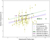 |
Fig. 1 Electron temperature as a function of the galactocentric radius. The lines in this graph are a fit to the sample of measuredelectron temperatures in our catalog in blue; the gradient determined by Balser et al. (2015) in red; the gradient determined by Paladini et al. (2004) in green. |
4.2 Rescaling to 74 MHz
To be able to compare the different datasets to each other we have rescaled all to 74 MHz. This frequency was chosen when we compiled Papers 1–3 into a catalog, as most of the data were already at 74 MHz. The 88 MHz data from Papers 4 and 5 were not added until later. To rescale brightness temperatures to a new frequency we have chosen a temperature spectral index of − 2.7. This value is also used in Papers 1, 3, and 4. Papers 2 and 5 use different values of − 2.55 and − 2.3, respectively. Other discussions of the temperature spectral index (specifically Strong et al. 2011 and references therein) provide spectral indices ranging from − 3.0 to − 2.3, for frequencies ranging between 80 MHz and 22 GHz. We considered − 2.7 to be a reasonable value since all but one of the emissivities stay within one sigma of each other when using any spectral index between − 2.3 and − 2.7. The outlier here still lies well within three sigma when using spectral index − 2.3 instead of − 2.7.
The temperature spectral index β is defined as T ∝ ν−β, the temperature at the new frequency
 (9)
(9)
where Tori is the foreground or background brightness temperature at the original frequency νori, T74 is the foreground or background brightness temperature at 74 MHz. The new emissivity is defined as
 (10)
(10)
where D is either DF or DB.
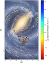 |
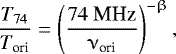
Fig. 2 Observed emissivities as a function of the HII region location in the Milky Way, plotted in a logarithmic color scale. HII regions with foreground emissivities (ϵF) are indicated with a triangle, background emissivities (ϵB) with circles. Background image: NASA/JPL-Caltech/ESO/R. Hurt. |
5 Analysis of observed emissivities
Figure 2 shows the emissivities, ϵ from the catalog overlaid on an artist’s concept of the Milky Way plane. Here the triangles indicate the foreground emissivities which show mostly high values of log ϵ > 0.6. These foreground emissivities are also shown in the left hand plot of Fig. 3 and are traced with HII regions rather close to the Sun (D < 2.5 kpc; Table A.1). We have attempted to use a local enhancement to explain these higher emissivity values, discussed in further detail in Sect. 6.2. The background emissivities in Figs. 2 and 3 show four noticeable features. Firstly, the general trend for HII regions behind the Galactic center (from our point of view) is to have mid range emissivities (log ϵ ≈ −0.3 to 0.0). These HII regions have path lengths between 14 and 17 kpc. Secondly, HII regions in front of the Galactic center (path lengths 22–26 kpc) feature mostly in low range emissivities (log ϵ < −0.3). Thirdly, six HII regions on the LOS in the direction (within a few degrees) of the Galactic center do not show the lower emissivity values of the surrounding HII regions, but have values of log ϵ ≈ 0.0–0.3, indicating an increase in the emissivities along those LOS. This is also shown in the zoom-in Fig. 4 (the six yellow and green circles close to the Sun). These HII regions have path lengths between 27 and 28 kpc. This might mean that there is a region with higher emissivity behind this group of HII regions but in front of any path lengths that do not show this elevated emissivity. We speculate that this could be caused by a localized feature of enhanced synchrotron emission in the Scutum-Centaurus arm. Fourthly, in the right-hand plot of Fig. 3, two data points from Paper 4 can be seen with slightly elevated emissivities. Considering the spatial location of these two HII regions, we conclude no deviating location: they are located within the 3D distribution of all HII regions. Therefore, it is deemed unlikely that their deviating measured values are real and caused by a local enhanced emissivity. Instead, it is suspected that the measurements may be overestimates of the real emissivities. These two HII regions in particular have an estimated surface comparable to the beam size. Therefore, possible contamination by background synchrotron emission cannot be excluded. Discarding these points would not make a significant change in the model fits.
Emissivity modeling equations.
6 Emissivity modeling
In a two-step attempt to model the catalog emissivities, we use simple axisymmetric emissivity models and detailed GMF-based emissivity models to describe the catalog emissivities.
6.1 Models
We employed a number of different models, as used in Papers 3 and 5, to simulate synchrotron emissivity and optimize their parameters by comparison to the observed emissivities, using least-squares minimization:
- 1.
constant emissivity;
- 2.
Gaussian decrease in synchrotron emissivity with galactocentric radius;
- 3.
exponential decrease in synchrotron emissivity with galactocentric radius;
- 4.
three zone model (TZM), consisting of concentric rings centered on the Galactic center, with varying emissivities.
The parameters for each model can be found in Table 3. The TZM is different from the others: its three emissivity values are optimized by the code, but the radii that divide these zones are fixed before the final optimization. The radii used here are chosen by running the existing optimization code with an extensive combination of radii. The R1–R2 combination that provides the best reduced chi-squared value is chosen. The best-fit results are shown in Fig. 5, and are discussed in Sect. 7.1.
In addition to these four models, we simulated Galactic emissivities using two different GMF models. Model J13b is based on the “J10” model from Jaffe et al. (2010), but the current parameters for the model come from Planck Collaboration Int. XLII (2016) where it was called “Jaffe13b”. Model JF12 is presented in Jansson & Farrar (2012). Both of these models are created using total intensity and polarized synchrotron emission maps and extragalactic rotation measures. Model J13b is a four armed logarithmic spiral model, with a molecular ring. Model JF12 has eight logarithmic spiral arm sections and a halo. Both models have a combination of coherent, random and ordered magnetic fields. The specific field strengths of all the components can be found in the references above. In general, higher synchrotron intensity is observed from a region with a magnetic field direction perpendicular to our LOS. In addition, a model of a constant CR density was assumed throughout the Galaxy. The results for these simulations are discussed in Sect. 7.2.
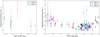 |
Fig. 3 Left panel: observed foreground emissivities (ϵF) as a function of the path length for Papers 1 and 2. Right panel: same as left panel, but for the observed background emissivities (ϵB) from Papers3–5. |
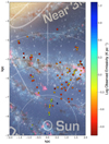 |
Fig. 4 A zoom-in of the Milky Way plot in Fig. 2. The dust band moving from coordinates [−2,−5] kpc and [+2,−6] kpc is the Scutum-Centaurus spiral arm. Background image: NASA/JPL-Caltech/ESO/R. Hurt. |
6.2 Enhancement in synchrotron emissivity in the Solar neighborhood
A local emissivity enhancement has been used in previous papers to explain enhanced synchrotron emissivity and is discussed in various papers (e.g. Sun et al. 2008; Fleishman & Tokarev 1995; Wolleben & Reich 2004). To explore any significant presence of an elevation in the foreground emissivities, we compare our catalog emissivities to a local emissivity as proposed by Beuermann et al. (1985) using a spectral index of − 2.7. Beuermann et al. (1985) use 408 MHz data (Haslam et al. 1982) to model the radio structure of our Galaxy and find a mean local emissivity of 0.011 ± 0.003 K pc−1, equal to 1.10 ± 0.30 K pc−1 at 74 MHz. This value is consistent within the error with the mean value we find for our foreground emissivities with distances within 1 kpc, which is 1.52 ± 0.99 K pc−1 at 74 MHz. This substantiates the need to model a local enhancement.
We followed the reasoning of Sun et al. (2008) and modeled an enhancement within 600 pc around the Sun. Exploring different enhancement values, we find that 1.2 K pc−1 would provide a good fit, based on the reduced chi-squared values (see Table 4 and Sect. 7.1). As explanation for a local enhancement, Sun et al. (2008) propose that there is either an enhanced local CR density or an increase of the local turbulent magnetic field, but they have not been able to distinguish between them.
7 Modeling results
In this section we discuss the results of the modeling effort with the simple axisymmetric emissivity models and the more complex GMF-based emissivity models.
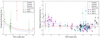 |
Fig. 5 Left panel: observed foreground emissivities (ϵF) as a function of the path length for papers 1and 2. Right panel: same, but for the observed background emissivities (ϵB) from Papers3–5. In both plots the simulated emissivities for the simple models are shown. In Sect. 7 we discuss the results of the modeling in detail. |
Emissivity modeling parameters.
7.1 Simple axisymmetric emissivity models
We compare the emissivities calculated in our models with the observed emissivities from our catalog. In Table 4 we present the resulting best-fit parameters. Considering the reduced chi-squared values from this table, we can expect that the constant, Gaussian and exponential model results hardly deviate from each other. The TZM shows a better fit in general, which is not unexpected as a more complex model is likely to fit better to complex data. The combination of modeled TZM emissivity values ϵ1 and ϵ2 is consistent with the assumption that the CR density follows the source density, while the higher outer emissivity ϵ3 does not follow this naive assumption. However, this model is still too simple for us to have much confidence in its results. These four models werefitted to both foreground and background simultaneously, the shown fits are constrained by all the data. For clarity we have split the foreground and background emissivities, including fits, in two plots in Fig. 5. For foreground emissivities the models follow the trend discussed in Sect. 5 well. All fits are consistent with the data, within the error. The constant, Gaussian and exponential models show roughly the same fit and are plotted on top of each other. The TZM falls slightly below the other models, but still within two sigma from each data point. There is no significant difference between the four models, and no model is significantly better than the rest. For the background emissivities, the path length spread of 14–28 kpc gives rise to more differences between the four models. Due to the high value of the β1 -parameter that determines the width of the bell and its even higher uncertainty, the Gaussian model is barely distinguishable from the constant model. The exponential model shows a negative slope when plotting emissivity values as a function of path length, and at shorter path lengths (from our point of view behind the Galactic center and close to the Galactic edge – see Sect. 7.2) shows elevated emissivity values. This is an interesting result, specifically regarding the GMF modeling in the next section. The exponential model does not show significant difference with respect to the constant and Gaussian models and does not fit to the observational data. The TZM is better at reproducing emissivity values compared to the other models. Nevertheless, we have to conclude that the Galactic structure cannot be reproduced by these simple axisymmetric emissivity models.
7.2 Galactic magnetic field models
Focussing on more astrophysically founded models, we use existing magnetic field models J13b and JF12. We used the software package HAMMURABI (Waelkens et al. 2009) to simulate synchrotron emissivities from the GMF and (non-astrophysical) constant CR density model.
As none of these magnetic field models take a local enhancement into account we only consider background emissivities in our analysis. The simulated data are not normalized to display emissivities at 74 MHz because the underlying magnetic field models have been based on synchrotron measurements at 22 and 94 GHz. Due to unknown variations in the synchrotron spectral index across the Milky Way, it is difficult to reliably extrapolate to 74 MHz. Therefore, in this paper we have treated the absolute flux level of the simulated data as unknown at 74 MHz. Assuming a constant spectral index for all sight lines, we can compare the general distribution of observed and simulated emissivities as a function of HII region position. We attempted an ad hoc normalization to the observational data by a least-squares minimizing method to be able to compare the different models and discern possible trends. It is difficult to determine if such a normalization is correct. To test multiple scenarios, we have performed two different normalizations. One scenario assumes that the data with long path lengths fit the model (Fig. 7), so that the simulated data sets are normalized with respect to the long path lengths (>18 Kpc). The second scenario assumes that the data with short path lengths fit the model (Fig. 8), so that the simulated data sets are normalized with respect to the short path lengths (<18 Kpc). For convenience all data sets have been binned. Although the correctness of the normalizations cannot be determined, different trends caused by the different magnetic field models can be studied.
Figure 7 shows a lower emissivity in models as compared to observations for path lengths between 14 and 20 kpc. We plot the location of the HII regions considered here in Fig. 6, which shows that path lengths between 14 and 18 kpc are located behind the Galactic center. This is the same subgroup of HII regions we discussed in Sect. 5, related to higher emissivities behind the Galactic center.
At longer path lengths and thus closer to the observer (see Fig. 6), we see that the simulated values are better able to reproduce the trend in the observed emissivities. This suggests that we would need a higher CR density or stronger magnetic field in the far outer Galaxy to explain these observations.
Figure 8 shows that an agreement of observed and simulated emissivities at the short path lengths gives rise to an overprediction of emissivity at the long path lengths. This can be explained with a lower magnetic field strength or CR underdensity in the central region of the Galaxy. The binned figures seem to suggest that a better fit is achieved for the long path length normalization in Fig. 7.
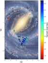 |
Fig. 6 HII regions in their assumed location in the Milky Way, with a color scheme based on their LOS path lengths. HII regions withbackground data only. Background image: NASA/JPL-Caltech/ESO/R. Hurt. |
8 Discussion
8.1 Comparison with previous work
One of the models put forward in Paper 3 is the constant emissivity model. Their conclusion that this model is unsuitable is reinforced with the additions of multiple data sets to the catalog. A constant type model can be fit to the data if we split the catalog up in subsets and try a model that has several different constant emissivities in different regions, exactly like the TZM. Expanding the number of regions in this model will allow a better fit, not unexpected as one increases the degrees of freedom. However, this type of model does not have a clear physical basis from which to explain any underlying distribution of CR density or magnetic field. It will likely also not explain the scatter in emissivities that we see in our sample.
The second model from Paper 3 is one where the inner 3 kpc region in the Galactic center has a CR underdensity and the rest of the Galactic plane has a constant emissivity. This model as a whole cannot be reproduced, moreover the simple models – specifically the TZM – only produce an overdensity in this region. However, the modeling results in Sect. 7.2 do show one of two scenarios that might call for the underdensity that Paper 3 has suggested.
In general terms, our conclusions about the simple axisymmetric emissivity models are similar to the conclusions in Paper 5. We can agree that these four models are much too simplified to explain all the features in the observations. In terms of the modeling parameters however, there is little overlap between them. Considering the use of additional data to that of Paper 5, these differences are expected. More complex models based on more than axisymmetry are needed.
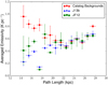 |
Fig. 7 Simulated data from the GMF-based emissivity models with the observed emissivities from the catalog. All data are averaged over bins of 1 Kpc width, as indicated by the horizontal error bars. For the model data, the vertical error bars indicate the variance in the binned data. A lack of vertical error bar indicates the presence of only one data point in the bin. Shown is the synchrotron emissivity (y-axis) as a functionof the path length for each HII region (x-axis). The simulated data shown here is normalized with respect to the longer path lengths (>18 Kpc). |
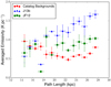 |
Fig. 8 Same as in Fig. 7, but the simulated data shown here is normalized with respect to the shorter path lengths (<18 Kpc). |
8.2 This work
Analyzing the results from Sect. 7, there are multiple scenarios that can play a role. In this section we try to substantiate these scenarios. With respect to the modeled emissivities, the observed emissivities in the region behind the Galactic center appear high (Fig. 7). This can be explained by introducing either a high magnetic field strength or a high CR density in the far outer region of the Milky Way. An elevated GMF strength for this scenario would likely be located in the far branch of the Scutum-Centaurus arm, and has to cover at least an area in direction of the Galactic center between Galactic longitudes 330° and 30°. Considering that the direction of the arm in the far outer Galaxy is perpendicular to our LOS, an increased GMF strength would indeed maximally increase the emissivity from this region. It cannot be determined whether this region of enhanced magnetic field would extend only over this region, or extend along the Scutum-Centaurus arm. However, if the entire spiral arm had an elevated field strength, this would have been apparent in the fit parameters of the J13b and JF12 models. In addition, our data does not show any evidence of enhanced magnetic field strength in the near crossing of the Scutum-Centaurus arm. Results by Beck (2015, their Fig. 3, and related text and references therein) suggest that at least one external galaxy (IC342) shows a higher magnetic field strength at outer radii. However, there is no indication that this is the case in the Milky Way. Figure 1 in Beck (2001) shows no elevated magnetic fields in the Milky Way as a function of Galactic radius. And considering the lack of Galactic CR accelerators in this part of the Galaxy, an elevated CR density is also not expected. Overall this first scenario seems unlikely.
The lower emissivities at longer path lengths (Fig. 8) can be achieved by either low magnetic field strength or a low CR density in the inner radii of the Galaxy. This scenario can be connected to Galactic winds that rapidly move CRs to other parts of the Galaxy from the Galactic center. Current Galactic wind models (e.g., Recchia et al. 2016; Taylor & Giacinti 2017) do not give any indication on what level of CR displacement is achieved. This scenario can also be connected to a possible X-shaped GMF (Ferrière & Terral 2014), where an additional removal of CRs is realized. It is uncertain at this time what the extent of the CR outflow will be, and if it will be sufficient. In Figure 6a in Beuermann et al. (1985) however, there is an indication that the emissivity does have a downward trend in the central radii of the Milky Way.
The third option is that none of the above scenarios are true, which is a reasonable assumption since the models are still very simple. Let us assume that the structure in CR density will give rise to variable spectral indices for the synchrotron emissivity. This implies that the constant spectral index value of − 2.7 we have used is incorrect for most regions of the sky. Consequently, using different spectral indices to rescale the different entries in our catalog, the current observed differences might disappear and with it the need to establish scenarios 1 and 2 above. In addition to a variable spectral index, we also need to consider the validity of using a radius of 20 kpc to describe the Galactic disk. These options will be explored in a forthcoming paper.
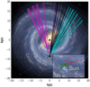 |
Fig. 9 Lines-of-sight for all HII regions in the catalog. Inset is a zoom-in of the foreground LOS that are close to the Sun. We show Paper 1 in red, Paper 2 in green, Paper 3 in magenta, Paper 4 in cyan, and Paper 5 in black. Background image: NASA/JPL-Caltech/ESO/R. Hurt. |
9 Conclusions
In this workwe have combined existing low-frequency observations of HII regions, with known distances in the Milky Way, into one catalog. We simulated the values in this catalog using different models. Using all these observations combined is advantageous, as the data are distributed over a larger area of the Milky Way than all the original data sets separately. This allows us to probe the emissionon much wider distance scales. This is especially important for the simple axisymmetric emissivity models, because the parameters need to be valid for a larger distribution than before. The simplicity of these models and the lack of a physical basis is their undoing, and much more detailed models are needed. One new feature in this work is the usage of existing GMF-based emissivity models to simulate Galactic synchrotron emission as one would observe it.
Our comparison shows that the inconsistencies between the simulated and observed data can be explained by any of the following scenarios:
- 1.
elevated CR density or magnetic field strength in the outer radii of the Milky Way;
- 2.
lower CR density or magnetic field strength in the inner radii of the Milky Way;
- 3.
a variable spectral index that changes the morphology of the current emission level distribution.
Due to a considerable body of work on both the magnetic field strength and the likely CR density in the outer regionof the Milky Way, the first scenario seems unlikely. The second and third scenarios however appear promising and will be discussed in upcoming paper(s), since theories of Galactic winds and X-shaped magnetic fields might provide a big enough outflow of CRs to cause a paucity in the inner region of the Galaxy. And considering the unlikely assumption of a constant spectral index in the entire Galaxy, new rescaled emissivities need to be calculated for the next version of our catalog. These new values can be used to revisit some of the modeling here.
10 Future work
As already set forth in Sects. 8 and 9, respectively, a non-constant spectral index is likely to change the distribution of the synchrotron emissivities in our collection. An important future venture is to use the measured spectral-index spread along the Milky Way to redo some of the modeling presented in this paper. It will be interesting to see the likely change in scenarios that are put forth by the modeling effort now.
Another interesting change in the current effort would be the Galactic boundary, which is currently set to 20 kpc. This value is the assumed boundary of the region emitting the bulk of the Galactic synchrotron emission. The actual value of the Milky Way boundary is unknown, although it is possible that CRs and magnetic fields will extend far beyond those 20 kpc (Levine et al. 2006). It would be an interesting exercise to quantify the changes with a different Galactic radius.
Considering the current conclusions and the suggested scenarios, it would be worthwhile to compare more GMF-based emissivity models. If a constant CR density model (such as the one in this paper) is used, the simulated synchrotron emissivity from many different GMF-based emissivity models can be compared to both the existing catalog and to each other. The different details for each GMF and their influence on the simulated emission can be discussed. Alternatively, more realistic CR distributions (e.g., GALPROP, Strong et al. 2009; DRAGON Maccione et al. 2011; PICARD, Kissmann 2014) can also provide interesting results when used in our simulations.
New emissivity values for HII regions with known distances can be added to the existing catalog, specifically from observations with the LOFAR instrument (van Haarlem et al. 2013). We hope to add HII regions from a signicant part of the Milky Way plane to the catalog, for example using results from the ongoing Low-Band Array surveys with LOFAR. The expanded catalog can be used for extended modeling of the Galactic synchrotron emissivity.
Acknowledgements
I.P. would like to acknowledge funding from the Netherlands Research School for Astronomy (NOVA). Cameron van Eck is thanked for his help and advice, specifically regarding modeling and plotting. This research made extensive use of NumPy (van der Walt et al. 2011); IPython (Perez & Granger 2007), and matplotlib (Hunter 2007).
Appendix A Additional table
Complete catalog of HII regions detected in absorption.
References
- Alves, M. I. R., Davies, R. D., Dickinson, C., et al. 2012, MNRAS, 422, 2429 [NASA ADS] [CrossRef] [Google Scholar]
- Anderson, L. D., Bania, T. M., Balser, D. S., et al. 2014, ApJS, 212, 1 [NASA ADS] [CrossRef] [Google Scholar]
- Azcárate, I. I. A. d. R., Cersósimo, J. I. A. d. R., & Colomb, F. I. A. d. R. 1990, Rev. Mex. Astron. Astrofis., 20, 23 [NASA ADS] [Google Scholar]
- Baars, J., Genzel, R., Pauliny-Toth, I., & Witzel, A. 1977, A&A, 61, 99 [NASA ADS] [Google Scholar]
- Balser, D. S., Wenger, T. V., Anderson, L. D., & Bania, T. M. 2015, ApJ, 806, 199 [NASA ADS] [CrossRef] [Google Scholar]
- Beck, R. 2001, Space Sci. Rev., 99, 243 [NASA ADS] [CrossRef] [Google Scholar]
- Beck, R. 2015, A&ARv, 24, 4 [NASA ADS] [CrossRef] [Google Scholar]
- Beuermann, K., Kanbach, G., & Berkhuijsen, E. M. 1985, A&A, 153, 17 [NASA ADS] [Google Scholar]
- Caswell, J. L. 1976, MNRAS, 177, 601 [NASA ADS] [Google Scholar]
- Costain, C. H., Lacey, J. D., & Roger, R. S. 1969, IEEE Trans. Antennas Propag., 17, 162 [NASA ADS] [CrossRef] [Google Scholar]
- Diesing, R., & Caprioli, D. 2018, Phys. Rev. Lett., 121, 091101 [NASA ADS] [CrossRef] [Google Scholar]
- Ferrière, K. 2016, J. Phys. Conf. Ser., 767, 012006 [CrossRef] [Google Scholar]
- Ferrière, K., & Terral, P. 2014, A&A, 561, A100 [NASA ADS] [CrossRef] [EDP Sciences] [Google Scholar]
- Finlay, E., & Jones, B. 1973, Aust. J. Phys., 26, 389 [NASA ADS] [CrossRef] [Google Scholar]
- Fleishman, G., & Tokarev, Y. 1995, A&A, 293, 565 [NASA ADS] [Google Scholar]
- Georgelin, Y. P., & Georgelin, Y. M. 1970, A&A, 6, 349 [NASA ADS] [Google Scholar]
- Grenier, I. A., Black, J. H., & Strong, A. W. 2015, ARA&A, 53, 199 [NASA ADS] [CrossRef] [Google Scholar]
- Haslam, C. G. T., Salter, C. J., Stoffel, H., & Wilson, W. E. 1982, A&AS, 47, 1 [NASA ADS] [Google Scholar]
- Hindson, L., Johnston-Hollitt, M., Hurley-Walker, N., et al. 2016, Publ. Astron. Soc. Aust., 33, e020 [Google Scholar]
- Humphreys, R. M. 1978, ApJS, 38, 309 [NASA ADS] [CrossRef] [EDP Sciences] [Google Scholar]
- Hunter, J. D. 2007, Comput. Sci. Eng., 9, 90 [NASA ADS] [CrossRef] [Google Scholar]
- Hurley-Walker, N., Callingham, J. R., Hancock, P. J., et al. 2017, MNRAS, 464, 1146 [NASA ADS] [CrossRef] [Google Scholar]
- Jaffe, T. R., Leahy, J. P., Banday, A. J., et al. 2010, MNRAS, 401, 1013 [NASA ADS] [CrossRef] [Google Scholar]
- Jansson, R., & Farrar, G. R. 2012, ApJ, 761, L11 [NASA ADS] [CrossRef] [Google Scholar]
- Jones, B., & Finlay, E. 1974, Aust. J. Phys., 27, 687 [NASA ADS] [CrossRef] [Google Scholar]
- Kassim, N. E. 1990, Lect. Notes Phys., 362, 144 [NASA ADS] [CrossRef] [Google Scholar]
- Kissmann, R. 2014, Astropart. Phys., 55, 37 [NASA ADS] [CrossRef] [Google Scholar]
- Levine, E. S., Blitz, L., & Heiles, C. 2006, Science, 312, 1773 [NASA ADS] [CrossRef] [Google Scholar]
- Maccione, L., Evoli, C., Gaggero, D., & Grasso, D. 2011, DRAGON: Galactic Cosmic Ray Diffusion Code, Astrophysics Source Code Library [Google Scholar]
- Mathewson, D. S., Broten, N. W., & Cole, D. J. 1965, Aust. J. Phys., 18, 665 [NASA ADS] [CrossRef] [Google Scholar]
- Mertsch, P., & Petrosian, V. 2017, Proc. Sci., 35, 1108 [Google Scholar]
- Mezger, P. G., & Henderson, A. P. 1967, ApJ, 147, 471 [NASA ADS] [CrossRef] [Google Scholar]
- Nord, M. E., Henning, P. A., Rand, R. J., Lazio, T. J. W., & Kassim, N. E. 2006, AJ, 132, 242 [NASA ADS] [CrossRef] [Google Scholar]
- Paladini, R., Burigana, C., Davies, R. D., et al. 2003, A&A, 397, 213 [NASA ADS] [CrossRef] [EDP Sciences] [Google Scholar]
- Paladini, R., Davies, R. D., & Dezotti, G. 2004, MNRAS, 347, 237 [NASA ADS] [CrossRef] [Google Scholar]
- Perez, F., & Granger, B. E. 2007, Comput. Sci. Eng., 9, 21 [Google Scholar]
- Planck Collaboration XXV. 2016, A&A, 594, A25 [NASA ADS] [CrossRef] [EDP Sciences] [Google Scholar]
- Planck Collaboration Int. XLII. 2016, A&A, 596, A103 [NASA ADS] [CrossRef] [EDP Sciences] [Google Scholar]
- Recchia, S., Blasi, P., & Morlino, G. 2016, MNRAS, 462, 4227 [NASA ADS] [CrossRef] [Google Scholar]
- Roger, R. S. 1969, ApJ, 155, 831 [NASA ADS] [CrossRef] [Google Scholar]
- Roger, R. S., Costain, C. H., Landecker, T. L., & Swerdlyk, C. M. 1999, A&A, 19, 7 [Google Scholar]
- Scheuer, P., & Ryle, M. 1953, MNRAS, 113, 4 [NASA ADS] [CrossRef] [Google Scholar]
- Shain, C. 1959, IAU [Google Scholar]
- Strong, A. W., Moskalenko, I. V., Porter, T. A., et al. 2009, ArXiv e-prints [arXiv:0907.0559] [Google Scholar]
- Strong, A. W., Orlando, E., & Jaffe, T. R. 2011, A&A, 534, A54 [NASA ADS] [CrossRef] [EDP Sciences] [Google Scholar]
- Su, M., Slatyer, T. R., & Finkbeiner, D. P. 2010, ApJ, 724, 1044 [NASA ADS] [CrossRef] [Google Scholar]
- Su, H., Hurley-Walker, N., Jackson, C. A., et al. 2016, MNRAS, 13, 1 [Google Scholar]
- Sun, X. H., Reich, W., Waelkens, A., & Enßlin, T. A. 2008, A&A, 477, 573 [NASA ADS] [CrossRef] [EDP Sciences] [Google Scholar]
- Taylor, A. M., & Giacinti, G. 2017, Phys. Rev. D, 95, 1 [Google Scholar]
- van der Walt, S., Colbert, S. C., & Varoquaux, G. 2011, Comput. Sci. Eng., 13, 22 [Google Scholar]
- van Haarlem, M. P., Wise, M. W., Gunst, A. W., et al. 2013, A&A, 556, A2 [NASA ADS] [CrossRef] [EDP Sciences] [Google Scholar]
- Waelkens, A., Jaffe, T., Reinecke, M., Kitaura, F. S., & Enßlin, T. A. 2009, A&A, 495, 697 [NASA ADS] [CrossRef] [EDP Sciences] [Google Scholar]
- Webber, W. R. 1977, ICRC, 1, 373 [NASA ADS] [Google Scholar]
- Wolleben, M., & Reich, W. 2004, A&A, 427, 537 [NASA ADS] [CrossRef] [EDP Sciences] [Google Scholar]
All Tables
All Figures
|
Fig. 1 Electron temperature as a function of the galactocentric radius. The lines in this graph are a fit to the sample of measuredelectron temperatures in our catalog in blue; the gradient determined by Balser et al. (2015) in red; the gradient determined by Paladini et al. (2004) in green. |
| In the text | |
|
Fig. 2 Observed emissivities as a function of the HII region location in the Milky Way, plotted in a logarithmic color scale. HII regions with foreground emissivities (ϵF) are indicated with a triangle, background emissivities (ϵB) with circles. Background image: NASA/JPL-Caltech/ESO/R. Hurt. |
| In the text | |
|
Fig. 3 Left panel: observed foreground emissivities (ϵF) as a function of the path length for Papers 1 and 2. Right panel: same as left panel, but for the observed background emissivities (ϵB) from Papers3–5. |
| In the text | |
|
Fig. 4 A zoom-in of the Milky Way plot in Fig. 2. The dust band moving from coordinates [−2,−5] kpc and [+2,−6] kpc is the Scutum-Centaurus spiral arm. Background image: NASA/JPL-Caltech/ESO/R. Hurt. |
| In the text | |
|
Fig. 5 Left panel: observed foreground emissivities (ϵF) as a function of the path length for papers 1and 2. Right panel: same, but for the observed background emissivities (ϵB) from Papers3–5. In both plots the simulated emissivities for the simple models are shown. In Sect. 7 we discuss the results of the modeling in detail. |
| In the text | |
|
Fig. 6 HII regions in their assumed location in the Milky Way, with a color scheme based on their LOS path lengths. HII regions withbackground data only. Background image: NASA/JPL-Caltech/ESO/R. Hurt. |
| In the text | |
|
Fig. 7 Simulated data from the GMF-based emissivity models with the observed emissivities from the catalog. All data are averaged over bins of 1 Kpc width, as indicated by the horizontal error bars. For the model data, the vertical error bars indicate the variance in the binned data. A lack of vertical error bar indicates the presence of only one data point in the bin. Shown is the synchrotron emissivity (y-axis) as a functionof the path length for each HII region (x-axis). The simulated data shown here is normalized with respect to the longer path lengths (>18 Kpc). |
| In the text | |
|
Fig. 8 Same as in Fig. 7, but the simulated data shown here is normalized with respect to the shorter path lengths (<18 Kpc). |
| In the text | |
|
Fig. 9 Lines-of-sight for all HII regions in the catalog. Inset is a zoom-in of the foreground LOS that are close to the Sun. We show Paper 1 in red, Paper 2 in green, Paper 3 in magenta, Paper 4 in cyan, and Paper 5 in black. Background image: NASA/JPL-Caltech/ESO/R. Hurt. |
| In the text | |
Current usage metrics show cumulative count of Article Views (full-text article views including HTML views, PDF and ePub downloads, according to the available data) and Abstracts Views on Vision4Press platform.
Data correspond to usage on the plateform after 2015. The current usage metrics is available 48-96 hours after online publication and is updated daily on week days.
Initial download of the metrics may take a while.