| Issue |
A&A
Volume 621, January 2019
|
|
|---|---|---|
| Article Number | A90 | |
| Number of page(s) | 10 | |
| Section | Cosmology (including clusters of galaxies) | |
| DOI | https://doi.org/10.1051/0004-6361/201834206 | |
| Published online | 15 January 2019 | |
Weak-lensing analysis of galaxy pairs using CS82 data
1
Instituto de Astronomía Teórica y Experimental, (IATE-CONICET), Laprida 854, X5000BGR Córdoba, Argentina
2
Observatorio Astronómico de Córdoba, Universidad Nacional de Córdoba, Laprida 854, X5000BGR Córdoba, Argentina
e-mail: This email address is being protected from spambots. You need JavaScript enabled to view it.
3
Centro Brasileiro de Pesquisas Físicas (CBPF), Rio de Janeiro, RJ 22290-180, Brasil
4
Instituto Argentino de Nivología, Glaciología y Ciencias Ambientales (IANIGLA-CONICET), Parque Gral San Martín, CC 330, CP 5500 Mendoza, Argentina
5
Departamento de Geofísica y Astronomía, CONICET, FCEFyN, UNSJ, Av. Ignacio de la Roza 590 (O), J5402DCS San Juan, Argentina
6
Brandeis University, 415 South Street, Waltham, MA 02453, USA
7
Shanghai Astronomical Observatory (SHAO), Nandan Road 80, Shanghai 200030, PR China
Received:
7
September
2018
Accepted:
11
November
2018
Abstract
Here we analyze a sample of close galaxy pairs (relative projected separation < 25 h−1 kpc and relative radial velocities < 350 km s−1) using a weak-lensing analysis based on the Canada-France-Hawaii Telescope Stripe 82 Survey (CS82). We determine halo masses for the total sample of pairs as well as for interacting, red, and higher-luminosity pair subsamples with ∼3σ confidence. The derived lensing signal for the total sample can be fitted either by a Singular Isothermal Sphere (SIS) with σV = 223 ± 24 km s−1 or a Navarro–Frenk–White (NFW) profile with R200 = 0.30 ± 0.03 h−1 Mpc. The pair total masses and total r band luminosities imply an average mass-to-light ratio of ∼200 h M⊙/L⊙. On the other hand, red pairs which include a larger fraction of elliptical galaxies, show a larger mass-to-light ratio of ∼345 h M⊙/L⊙. Derived lensing masses were compared to a proxy of the dynamical mass, obtaining a good correlation. However, there is a large discrepancy between lensing masses and the dynamical mass estimates, which could be accounted for by astrophysical processes such as dynamical friction, by the inclusion of unbound pairs, and by significant deviations of the density distribution from SIS and NFW profiles in the inner regions. We also compared lensing masses with group mass estimates, finding very good agreement with the sample of groups with two members. Red and blue pairs show large differences between group and lensing masses, which is likely due to the single mass-to-light ratio adopted to compute the group masses.
Key words: galaxies: interactions / galaxies: groups: general / gravitational lensing: weak
© ESO 2019
1. Introduction
Studies of galaxy pairs are important in order to understand the formation of massive galaxies and groups. Galaxy interactions in these systems are very common and play a significant role in galaxy evolution (e.g., Woods & Geller 2007; Ellison et al. 2010; Mesa et al. 2014) through their ability to produce galaxy morphology transformations (Toomre & Toomre 1972; Barnes & Hernquist 1992; Hopkins et al. 2008). For instance, the presence of a close galaxy companion drives a clear enhancement in galaxy morphological asymmetries, and this effect is statistically significant up to projected separations of at least < 50 h−1 kpc (Patton et al. 2016). Also, interacting galaxy pairs show physical effects generated by interactions that can be detected at large projected separations, as far as ∼150 kpc (Patton et al. 2013). These effects include enhancement of the star formation rate (Ellison et al. 2008, 2010; Patton et al. 2011, 2013; Scudder et al. 2012; Lambas et al. 2012) and active galactic nucleus (AGN) production (Barnes & Hernquist 1991; Hopkins et al. 2008; Darg et al. 2010), since it has been shown that the fraction of AGNs is larger for galaxies in pairs (Alonso et al. 2007). Despite the importance and prevalence of galaxy mergers in driving galaxy evolution, the physical details of the merging process are not yet fully understood even in the local universe.
Mass determinations of halos hosting galaxy pairs can contribute to a better understanding of galaxy evolution. A dynamical approach is commonly applied to estimate the mass enclosed by the galaxies. Nevertheless, determining the virial masses is very difficult for these systems given that the only available information is the velocity difference along the line-of-sight and the projected distance between the galaxies. Given the limitations, various methods have been proposed (Nottale & Chamaraux 2018; Chengalur et al. 1996; Peterson 1979; Faber & Gallagher 1979); recovering the mass however remains very uncertain.
Gravitational lensing allows us to derive the total projected mass distribution directly without relying on visible tracers. Strong lensing in particular provides information on the inner regions of galaxy systems (e.g., Collett et al. 2017; Cerny et al. 2018; Jauzac et al. 2018) and galaxies (e.g., van de Ven et al. 2010; Dutton et al. 2011; Suyu et al. 2012). Shu et al. (2016) applied this technique to model the mass distribution of a galaxy pair lens system, obtaining significant spatial offsets between the mass and light of both lens galaxies, which could be related to the interactions between the two lens galaxies. On the other hand, weak gravitational lensing is a powerful statistical tool that provides information regarding the projected mass distribution of galaxy systems at larger distances.
In particular, stacking techniques allow one to study low-mass galaxy groups and to derive the properties of the combined systems (e.g., Leauthaud et al. 2010; Melchior 2013; Rykoff et al. 2008; Foëx et al. 2014; Chalela et al. 2017, 2018). This technique has also been successfully applied to measure the mean masses of dark-matter halos for stacked samples of isolated galaxies (e.g., Mandelbaum et al. 2006; van Uitert et al. 2011; Schrabback et al. 2015; Charlton et al. 2017). Therefore, weak gravitational lensing is useful to study the dark-matter halos of a wide range of masses and can be applied to analyze the total mass content of galaxy pair systems.
In this work we analyze a sample of close galaxy pairs with a relative projected separation, rp, smaller than 25 h−1 kpc and relative radial velocities ΔV < 350 km s−1. This enhances the likelihood that the pair is physically associated as it reduces the number of pairs identified due to projection effects (Alonso et al. 2004; Nikolic et al. 2004; Edwards & Patton 2012). Also Kitzbichler & White (2008) identified close pairs in mock galaxy catalogues within Λ-CDM cosmological simulations, finding that most pairs identified with a projected separation rp ≤ 25 h−1 kpc and radial velocity difference ΔV < 300 km s−1 are physically close and will merge in an average time of ∼2 Gyrs. Moreover, at larger separations (rp > 100 kpc) it is important to consider the competing influences of other neighboring galaxies (Moreno et al. 2013; Karman et al. 2015) and larger-scale environmental influences (Park et al. 2007; Moreno et al. 2013; Sabater et al. 2013). We derive total masses through weak lensing using the Canada-France-Hawaii Telescope Stripe 82 Survey (CS82, Erben et al., in prep.) for different galaxy pair samples. Derived masses are compared to an indicative dynamical mass and with masses obtained from a galaxy group catalog computed according to the mass-to-light ratio. The work is organized as follows: in Sect. 2 we describe the sample of galaxy pairs. In Sect. 3 we give the details of the lensing analysis. In Sect. 4 we present the obtained masses, the mass-to-light ratios for the different galaxy pair samples analyzed, and the comparison to other mass estimates. Finally, in Sect. 5 we summarize and discuss the results. We adopt when necessary a standard cosmological model with H0 = 70 km s−1 Mpc−1, Ωm = 0.3, and ΩΛ = 0.7.
2. Galaxy pair sample
The sample of galaxy pairs is obtained from a redshift extended version of the Galaxy Pair Catalog (GPC; Lambas et al. 2012) based on the seventh data release of the Sloan Digital Sky Survey (SDSS-DR7; Abazajian et al. 2009). This survey comprises 11,663 square degrees of sky imaged in five wave-bands (u, g, r, i and z) containing photometric parameters of 357 million objects. The spectroscopic survey is a magnitude -limited sample to rlim < 17.77 (Petrosian magnitude) and most of the galaxies span a redshift range 0 < z < 0.25 with a median redshift of 0.1 (Strauss 2002).
Pair members are selected by requiring rp < 25 h−1 kpc and ΔV < 350 km s−1 (where rp is the relative projected separation between the galaxies and ΔV is the line-of-sight relative velocity). We perform a visual inspection of SDSS images to remove false identifications as described in Lambas et al. (2012). In order to obtain a larger sample and increase the signal-to-noise ratio (S/N) for the lensing analysis, we extended the original GPC up to z = 0.2, applying the same identification criteria.
With the aim of discarding pairs embedded in larger virialized structures as groups and clusters we use the redMaPPer v6.3 members catalog (redMaPPer catalogs, Rykoff et al. 2014). This catalog was obtained by the photometric cluster-finder algorithm redMaPPer (red-sequence Matched-filter Probabilistic Percolation), that identifies galaxy clusters as overdensities of red-sequence galaxies around spectroscopically identified central galaxy candidates. In order to compare GPC pairs with the members catalog we restrict the sample to pairs with z > 0.08. The discarded pairs are less than 5%. It is worth noting that this criterion only discards galaxy pairs in evolved systems with a defined red-sequence.
Magnitudes are calibrated using K-corrections of the publicly available code described in Blanton & Roweis (2007). To select pairs comprised by galaxies with similar individual stellar masses we consider an upper limit for the magnitude difference between the galaxy members,  , where
  and
and  are the absolute magnitudes in r-band of the brightest and the second brightest galaxy. The final catalog includes 1911 galaxy pairs in the SDSS-DR7 region ranging from redshift 0.08 to 0.2.
In order to perform the lensing analysis we select the pairs that are included in the CS82 area. The total sample includes 388 pairs. A larger density of pairs is located in the CS82 footprint since more spectroscopic information was available in this field at the time when the catalog was built. According to the visual inspection scheme described in Lambas et al. (2012), pairs are classified considering the interaction between the members into three categories: pairs undergoing merging, M; pairs with evident tidal features, T; and nondisturbed pairs, N. In this work we consider N pairs as noninteracting and we combine T and M pairs as interacting pairs. This visual classification by eye was performed by one of the authors in order to maintain a unified criteria. The reliability of this procedure was addressed by the comparison with the classification of a subsample of pairs by another author. We then estimated the classification uncertainty, obtaining ≲4%, according to the differences between the classifications by both authors in the same subsample. The purity of the catalog is therefore guaranteed by the process of visual inspection, in particular for the T and M systems with evidence of physical interaction.
We also classified galaxy pairs into red and blue pairs considering their position in the color-magnitude diagram (CMD; Fig. 2) and into higher luminosity and lower luminosity, according to their total r−band luminosity. Pairs with luminosities above the median of the total sample define the higher-luminosity subsample and conversely for the lower-luminosity one. Redshift, rp and ΔV distributions for the samples considered for the lensing analysis are shown in Fig. 1. As can be seen, interacting pairs tend to have lower rp distances than noninteracting systems. On the other hand, rp distributions for red and blue pairs, as well as higher- and lower-luminosity pairs, are all consistent with the total sample rp distribution. The total number of pairs in each subsample is presented in Table 1 for the total SDSS-DR7 region and for the pairs included in the CS82 masked area.
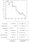 |
Fig. 1. Upper panel: redshift distribution of the total sample of galaxy pairs. Lower panel: median projected distances, Me(rp), and median radial velocity difference, Me(ΔV), for the different galaxy pair classes. Error bars corresponds to the standard deviations of rp and ΔV distributions obtained for each class. Noninteracting pairs tend to have larger rp distances than interacting pairs. On the other hand, rp distributions for red and blue pairs, as well as higher- and lower-luminosity pairs, are all in agreement with the total sample rp distribution. |
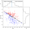 |
Fig. 2. Red and blue pairs classification criterion (central panel): Mg − Mr vs. Mr, where Mg and Mr are the total absolute magnitudes of the pairs in g−band and r−band, respectively. We divide the sample into 10 percentiles in magnitude Mr and then we compute the median color in each percentile (black dots). Subsequently, we fit a linear function (black line) to the obtained points and select the pairs with larger colors as red pairs and with lower colors as blue pairs. Upper and lower panels: total absolute magnitude and total color distributions of the pairs. The vertical blue line in the absolute magnitude distribution corresponds to the median value of this distribution, which is considered to classify higher- and lower-luminosity pairs. |
Number of galaxy pairs in each sample included in the SDSS-DR7 area and in the CS82 masked area.
3. Weak-lensing analysis
We use the same shear catalog and stacking technique as in Chalela et al. (2018). The shear catalog is based on the CS82 Survey, which is a joint Canada-France-Brazil project designed with the goal of complementing existing Stripe 82 SDSS ugriz photometry with high-quality i′−band imaging suitable for weak and strong lensing measurements. This survey is built from 173 MegaCam i′−band images and corresponds to an effective area of 129.2 degrees2, after masking out bright stars and other image artifacts. It has a median point spread function (PSF) of 0.6″ and a limiting magnitude i′≈24 (Leauthaud et al. 2017). Shear catalogs were constructed using the same weak lensing pipeline developed by the CFHTLenS collaboration using the lensfit Bayesian shape measurement method (Miller et al. 2013). Further details regarding the lensing catalog can be found in Leauthaud et al. (2017), Shan et al. (2017), Pereira et al. (2018), Chalela et al. (2018), for example.
Background galaxies, that is, galaxies affected by the lensing effect, are selected according to the Soo et al. (2018) photometric redshift catalog. We select galaxies with Z_BEST > zp + 0.1 and ODDS_BEST ≥0.6, where zp is the galaxy pair redshift, according to the average redshift of the galaxies, Z_BEST is the photometric redshift provided by Soo et al. (2018), and ODDS_BEST expresses the quality of the redshift estimates as being from 0 to 1.
In order to perform the lensing study we apply a stacking analysis to increase the signal. We summarize this technique in this subsection since it is described in detail in previous works (e.g., Gonzalez et al. 2017; Chalela et al. 2017, 2018). The weak gravitational lensing effect can be characterized by two quantities, the convergence κ, which accounts for the isotropic stretching of source images, and an anisotropic distortion given by the complex-value lensing shear, γ = γ1 + iγ2. The tangential component of the shear is related to the surface mass density, Σ(r), through (Bartelmann 1995):
 (1)
(1)
where we define the density contrast,  . Here,
  is the averaged tangential component of the shear in a ring of radius r,
  and
and  are the average projected mass distribution within a disk and in a ring of radius r, respectively, and Σcrit is defined below (Eq. (3)). On the other hand, the cross-component of the shear, γ×, defined as the component tilted at π/4 relative to the tangential component, should be zero. We can obtain an unbiased estimate of the shear as: ⟨e⟩≈γ, where ⟨e⟩ is the averaged ellipticity of background galaxies in annular bins.
The stacking methodology consists in considering a number of systems to derive the average mass. By combining several lenses, the density of the source galaxies is artificially increased. The density contrast is obtained as the weighted average of the tangential ellipticity of background galaxies of the lens sample:
 (2)
(2)
where ωLS, ij is the inverse variance weight computed according to the weight, ωij, given by the lensfit algorithm for each background galaxy,  . NLenses is the number of lensing systems and NSources, j the number of background galaxies located at a distance r ± δr from the jth lens. Σcrit, ij is the critical density for the ith source of the jth lens, defined as:
 (3)
(3)
Here, DOL, j, DOS, i and DLS, ij are the angular diameter distances from the observer to the jth lens, from the observer to the ith source and from the jth lens to the ith source, respectively. These distances are computed according to the adopted redshift for each galaxy pair (lens) and for each background galaxy (source). G is the gravitational constant and c is the light speed.
Once the density contrast is computed, we take into account a noise bias factor correction as suggested by Miller et al. (2013), which considers the multiplicative shear calibration factor m(νSN, l) provided by lensfit. For this correction we compute:
 (4)
(4)
following Velander et al. (2014), Hudson et al. (2015), Shan et al. (2017), Leauthaud et al. (2017), Pereira et al. (2018). Then, we calibrate the lensing signal as:
 (5)
(5)
The projected density contrast profile is computed using nonoverlapping concentric logarithmic annuli to preserve the S/N of the outer region, from  kpc (where the signal becomes significantly positive) up to
  Mpc.
Mpc.
Considering results regarding miscentering presented in Chalela et al. (2017), we adopt a luminosity weighted center according to the r−band galaxy member luminosity. Therefore, the center coordinates are obtained as
 (6)
(6)
where RA and Dec are the celestial coordinates, L is the r−band luminosity, and the sub-indexes 1 and 2 refer to the brightest and the second-brightest galaxy pair components, respectively. We tested the center selection by computing the profiles using as centers the brightest galaxy, RA1, Dec1, and a geometrical center, RA0 = (RA1 + RA2)×0.5, Dec0 = (Dec1 + Dec2)×0.5); we did not obtain significant differences between the results. This could be accounted for by the adopted inner radius ( kpc), which is approximately three times larger than the galaxy separation, which mitigates any bias introduced by the center selection.
We considered different logarithm bins, choosing between a total of seven and nine radial bins. We did not observe differences in the density profile parameters, within their uncertainties, among these choices, and therefore we fix the binning in order to obtain the lowest χ2 value. Given that the uncertainties in the estimated lensing signal are expected to be dominated by shape noise, we do not expect a noticeable covariance between adjacent radial bins and so we treat them as independent in our analyses. Accordingly, we compute error bars in the profile by bootstrapping the lensing signal using 100 realizations.
We tested whether or not the Z_BEST > zp+0.1 selection criterion was sufficient to discard foreground or weak satellite galaxies considering the large uncertainties in the photometric redshifts. Therefore, following Leauthaud et al. (2017) we computed the weak lensing profile for the total sample, with different lens-source separation cuts (Z_BEST > zp + 0.1, Z_BEST > zp + 0.2, Z_BEST > zp + 0.3 and Z_BEST > zp + 0.4). No statistically significant systematic trend was found in this test.
4. Results and discussion
4.1. Mass profile of stacked galaxy pairs
We model the derived density contrast profile of galaxy pairs using a Singular Isothermal Sphere (SIS) model and a Navarro–Frenk–White (NFW) profile (Navarro et al. 1997). The spherically symmetric NFW profile is derived from numerical simulations, according to the density, averaged over spherical shells, of dark-matter halos. This profile depends on two parameters, R200, which is the radius that encloses a mean density equal to 200 times the critical density of the universe, and a dimensionless concentration parameter, c200. This density profile is given by:
 (7)
(7)
where ρcrit is the critical density of the universe at the average redshift of the lenses, rs is the scale radius, rs = R200/c200 and δc is the characteristic overdensity of the halo:
 (8)
(8)
The mass within R200 can be obtained as M200 = 200 ρcrit-pagination  . Lensing formulae for the NFW density profile were taken from Wright & Brainerd (2000). If both R200 and c200 are taken as free parameters to be fitted, we obtain significantly large uncertainties in c200 values due to the lack of information on the mass distribution near the lens center. To overcome this problem, we follow van Uitert et al. (2012), Kettula et al. (2015) and Pereira et al. (2018), using a fixed mass-concentration relation c200(M200, z) derived from simulations by Duffy et al. (2008):
 (9)
(9)
where we take z as the mean redshift value of the lens sample. The particular choice of this relation does not have a significant impact on the final mass values, which have uncertainties dominated by the noise of the shear profile.
The SIS profile is the simplest density model for describing a relaxed massive sphere with a constant isotropic one-dimensional velocity dispersion, σV. At galaxy scales, dynamical studies (e.g., Sofue & Rubin 2001), as well as strong (e.g., Davis et al. 2003) and weak (e.g., Brimioulle et al. 2013) lensing observations, are consistent with a mass profile following approximately an isothermal law. The shear, γ(θ), and the convergence, κ(θ), at an angular distance θ from the lensing system center are directly related to σV by:
 (10)
(10)
where θE is the critical Einstein radius defined as:
 (11)
(11)
Therefore,
 (12)
(12)
We compute the mass within R200, following Leonard & King (2010):
 (13)
(13)
where H(z) is the redshift-dependent Hubble parameter. This equation is derived by equating 200ρc with the median density computed inside a spherical volume with radius R200.
To derive the parameters of each mass model profile we perform a standard χ2 minimization:
 (14)
(14)
where the sum runs over the N radial bins of the profile and the model prediction p refers to either σV for the SIS profile, or R200 in the case of the NFW model. Errors in the best-fitting parameters are computed according to the variance of the parameter estimates.
4.2. Total masses of galaxy pairs
Derived density contrast profiles for each sample are shown in Fig. 3 together with the fitted SIS and NFW models. The lower-luminosity sample is consistent with no signal (M200 masses are poorly determined with 1σ confidence) and is not shown in the figure. This sample is therefore removed from the rest of the analysis. In Table 2 we show the derived parameters. We could determine, with ∼3σ confidence, masses for the total sample and for interacting, red, and higher-luminosity pairs. Moreover, there is a significant difference of derived masses between higher- and lower-luminosity pairs, since galaxy pairs with larger luminosity are more massive systems. Noninteracting galaxy pairs tend to have lower total luminosities than interacting pairs which is in agreement with the lower lensing mass determined for noninteracting pairs. On the other hand, red pairs are more evolved systems since this sample includes more elliptical members. Hence, it is expected that these systems have larger masses than blue pairs, as is observed from the lensing analysis.
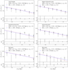 |
Fig. 3. Average density contrast profiles obtained for the analyzed galaxy pairs samples. h70 corresponds to h = 0.7. |
Results of the lensing analysis of galaxy pairs.
According to the derived masses we compute the mass-to-light ratio for the analyzed samples (Fig. 4). We consider the median luminosity according to the r−band absolute magnitude, Me(L). We obtain for the total sample a M200/Me(L)∼200 h M⊙/L⊙. This value is in agreement with mass-to-light ratio determinations for groups with similar masses to the analyzed pairs (Proctor et al. 2011; Girardi et al. 2002). Derived M200/Me(L) values for interacting, noninteracting and higher-luminosity pairs are in agreement with the derived value for the total sample. On the other hand, red pairs show a larger M200/Me(L), since this sample includes a larger fraction of elliptical members. It can be noticed from Fig. 4 that both lensing mass estimates, SIS and NFW, are in excellent agreement, indicating that the available data do not allow us to distinguish between the fitted models.
 |
Fig. 4. Mass-to-light ratios for the analyzed samples. Masses are the M200 derived according to the lensing analysis, considering SIS (crosses) and NFW (squares) models. Luminosity is computed according to r−band absolute magnitudes, adopting the median of the luminosity distribution for each sample. |
4.3. Comparison with dynamical estimates
In order to compare our mass determinations to dynamical estimates, we analyze the relation between our lensing results and an indicative mass, defined as (Faber & Gallagher 1979):
 (15)
(15)
which is related to the dynamical mass of a pair of objects in relative Keplerian motion. This parameter has been used to estimate the total mass enclosed within rp, although several assumptions regarding galaxy orbits are required (Nottale & Chamaraux 2018). Also, this approach considers that the pair is isolated and lacks dynamical friction effects. This is not entirely accurate since the large-scale structure has significant effects on the dynamics of galaxy pairs (Moreno et al. 2013; Mesa et al. 2018) and variations of the internal structure of the galaxies can modify their center of mass motion.
We derive the masses within a radius Me(rp)/2 (where Me(rp) is the median value of the projected distances derived for each sample) using the lensing results. The SIS mass inside a three-dimensional radius Me(rp)/2 is (Wright & Brainerd 2000):
 (16)
(16)
The NFW mass is obtained by:
 (17)
(17)
where ρ(r) is computed according to Eq. (7). The results are shown in Table 2. As expected, given that the SIS profile is steeper than the NFW profile, SIS masses within Me(rp)/2 are significantly larger than the NFW determinations.
In Fig. 5 we show the relation between MSIS(r < Me(rp)/2) and MNFW(r < Me(rp)/2) masses and the median values of F(MT) for each sample.
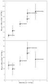 |
Fig. 5. Derived lensing masses compared to the median F(MT) defined according to Eq. (15), for the different galaxy pair samples. |
It is worth noting that the SIS and NFW mass profile parameters are obtained from the lensing signal at significantly larger radii compared to rp. Therefore, the masses extrapolated down to rp will be highly dependent on the assumed profile, as can be seen in the figure. In any case, there is a clear correlation between the indicative mass and the lensing masses at rp. We find that SIS masses are approximately five times the median F(MT) values while NFW masses are roughly half of F(MT). The indicative dynamical mass is expected to set a lower limit for the dynamical mass inside rp. Therefore, taken at face value, these results would favor the SIS profile compared to the NFW one, or could point to another scaling at small radii. In any case, astrophysical processes in interacting pairs, as well as the inclusion of gravitationally unbound pairs in the sample, can significantly bias dynamical estimates. Further analysis, including virial mass determinations considering the probability distribution for the projected rpΔV2 value, and a comparison with other density distribution models would be important to deepen our understanding of the mass distribution in close galaxy pairs.
4.4. Comparison with Yang groups
In this section we compare derived lensing masses with those available in a galaxy group catalog, in order to validate our results with other independent determinations. We chose to compare our mass estimates with group masses determined by Yang et al. (2012). We select this catalog given our experience with these galaxy systems (Rodriguez et al. 2015; Gonzalez et al. 2017) but mainly because it has reliable groups with low numbers of members. This group catalog was constructed using the adaptive halo-based group finder presented in Yang et al. (2005), updated to SDSS DR7. The idea of this algorithm is to assign galaxies into groups according to their common dark-matter halo. We refer the reader to Yang et al. (2005) for a complete description of the method and to Campbell et al. (2015) for a brief description and a deep analysis of the resulting groups identified by this algorithm.
For our comparison, it is important to take into account that the group mass is assigned according to a luminosity ranking and using an iterative relation between mass and luminosity. For this assignment, this method requires knowledge of the halo mass function and assumes the existence of a one-to-one relation between mass and luminosity for a given comoving volume and a given halo mass function. Group masses have a scatter of approx 0.3 dex (Yang et al. 2007) and, as pointed out by Campbell et al. (2015), the applied method is fundamentally limited in two ways: (i) the intrinsic scatter in the relation between group luminosity and halo mass; (ii) any errors in group membership determination will generally result in errors in group luminosity, and thus in the inferred halo mass. In particular, regarding the membership allocation errors, two failure modes are associated with this step: fragmentation and merging. Fragmentation refers to galaxies of the same group that are fractured into two or more groups, while merging refers to galaxies of separate groups that are assigned to one group.
In order to carry out the comparison we use galaxy pairs, covering the total SDSS-DR7 imaging area, described in Sect. 2. The sample includes 1911 pairs, of which 1656 have at least one galaxy that is identified as a member of a group. Of the 1911 pairs, 1177 have both galaxies identified in the same group. Furthermore, 95% of the pairs of this sample are in systems with less than ten members, while ∼60% (706 pairs) are identified in groups with only two members. This may be due to errors regarding membership allocation to the identified groups and/or because GPC includes galaxy pairs that are not isolated and are members of larger systems. For lower-mass systems, merging is more important in the membership assignment than fragmentation. This results in overestimates of group masses. On the other hand, nonisolated pairs located near the center of the groups bias the lensing signal to larger values and therefore larger mass estimates. In Fig. 6 we show the median distances of the pair center to the group center according to the number of members; pairs are at a median distance from the group center of lower than 0.35 × R180, where R180 is computed according to the halo group masses and is the radius that encloses a mean density equal to 180 times the critical density of the universe. Hence, pairs are mainly located near the group centers.
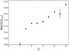 |
Fig. 6. Median distances of the pairs scaled with the radius, R180, to the group centers, according to the group number of members identified, Ng. Error bars are computed according to the root-mean-square deviation. For these systems, median R180 values range from 400 kpc to 1 Mpc. |
In Fig. 7 we show the lensing SIS masses compared to median group masses, Mg, computed by Yang et al. (2012) for each sample. In the left panel we show the comparison considering the groups that hold the two galaxies of the pair and have less than ten identified members. Median group masses are biased toward larger values (⟨Mg − M200⟩=4 × 10¹² h−1 M⊙) indicating that merging in the membership assignment could play an important role. In the right panel we compare the masses considering only groups that include both galaxies and have only two members; a good agreement is obtained for this relation (⟨Mg − M200⟩= − 0.44 × 10¹² h−1 M⊙). Although groups with low and intermediate masses have large uncertainties in their mass determinations, the median value for the total sample is in excellent agreement with the lensing estimate. For this sample, larger differences are observed for red and blue pairs, which could be due to the intrinsic scatter in the relation between group luminosity and halo mass. Since group masses are determined considering a noncolor-dependent mass-to-light ratio, this could bias mass determinations. As was shown in Fig. 4, red and blue pairs show differences with the derived M⊙/L⊙ compared to the other samples, therefore halo mass determinations for individual groups with a low number of galaxy members might be biased according to their color.
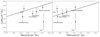 |
Fig. 7. Derived SIS lensing masses (M200) compared to the median masses derived by Yang, for the correlated pairs (left panel) and restricting the sample to pairs in groups with only two members (right panel). The solid black line corresponds to the identity function. |
5. Summary and conclusions
In this work we present a lensing analysis of galaxy pairs using weak lensing techniques. We determined lensing masses for different samples selected according to pair luminosity, color, and visual signatures of interaction. The derived mass-to-light ratios for the different samples are in agreement with ∼200 h M⊙/L⊙, except for the color-selected samples, where the red pair sample shows a larger mass-to-light ratio than blue pairs. This is in agreement with other works that report a correlation between dynamical mass-to-light ratios and colors for individual galaxies (Zandivarez & Martínez 2011; van de Sande et al. 2015), consistent with the fact that a galaxy M/L ratio strongly depends on age, metallicity, and stellar initial mass function. Furthermore, according to Wang & Brunner (2014), galaxy pairs composed of two early-type galaxies reside in high-mass halos and are often associated to more massive filaments (Mesa et al. 2018).
Derived lensing masses of interacting pairs are also significantly larger than the masses of non-interacting pairs. The inclusion of line-of-sight pairs in the latter could bias mass estimates to lower values, since truly bound galaxy systems tend to reside in more massive halos than isolated galaxies.
Lensing masses obtained within the median projected distance of the galaxies for each sample were compared to an indicative of the dynamical mass, F(MT). Due to projection effects, this parameter provides a lower limit of the dynamical mass enclosed by the galaxy pair. There is a clear correlation between F(MT) and lensing-derived NFW and SIS model masses. However, assuming an NFW profile, lensing masses are ∼50% lower than F(MT), while SIS masses exceed F(MT) values by a factor of approximately five. Astrophysical processes taking place in interacting systems could bias the projected relative velocity toward low values, leading to underestimates of the dynamical mass. In particular, dynamical friction drives orbital angular momentum transfer into the internal regions of halos (Gabbasov et al. 2014). On the other hand, gravitationally unbound pairs would result in larger ΔV values. Also, it is important to take into account that the derived lensing parameters are obtained from the projected density distribution of the halo at considerably larger radii compared to the projected distance between the galaxies. Therefore, significant deviations of the density distribution from single NFW and SIS profiles could be present.
We also compare lensing masses with Yang et al. (2012) group determinations. We notice that erroneously merged groups resulting in incorrect membership allocation might strongly bias the group masses toward high values. Nevertheless, when the group sample is restricted to galaxy systems with only two members, very good agreement between the lensing estimates and group masses is obtained. Although red and blue pairs show large differences between group and lensing masses, we remark that this is likely to be caused by a single mass-to-light ratio adopted by Yang et al. (2012), regardless of galaxy color.
Galaxy pairs are the simplest systems that can provide valuable information on galaxy morphology transformations. They are also important in galaxy group and cluster formation since pairs are formed at the center of more massive dark-matter halos than single galaxies (Wang & Brunner 2014). In this work we derive lensing masses for a sample of close pairs and we find that red pairs show larger masses and higher mass-to-light ratios. In a future work we plan to constrain the derived results with hydrodynamical simulations in order to explore galaxy formation and evolution scenarios. The study of these galaxy systems will contribute to a better understanding of galaxy transformation and group formation.
Acknowledgments
The authors thank the anonymous referee for their useful comments, which helped to improve this paper. This work was partially supported by the Consejo Nacional de Investigaciones Científicas y Técnicas (CONICET, Argentina), the Secretaría de Ciencia y Tecnología de la Universidad Nacional de Córdoba (SeCyT-UNC, Argentina), the Secretaría de Ciencia y Técnica de la Universidad Nacional de San Juan, the Brazilian Council for Scientific and Technological Development (CNPq) and the Rio de Janeiro Research Foundation (FAPERJ). We acknowledge the PCI BEV fellowship program from MCTI and CBPF. MM acknowledges the hospitality of Fermilab. Otag Icram. Fora Temer. This work is based on observations obtained with MegaPrime/MegaCam, a joint project of CFHT and CEA/DAPNIA, at the Canada-France-Hawaii Telescope (CFHT), which is operated by the National Research Council (NRC) of Canada, the Institut National des Sciences de l’Univers of the Centre National de la Recherche Scientifique (CNRS) of France, and the University of Hawaii. The Brazilian partnership on CFHT is managed by the Laboratório Nacional de Astrofísica (LNA). We thank the support of the Laboratório Interinstitucional de e-Astronomia (LIneA). We thank the CFHTLenS team for their pipeline development and verification upon which much of the CS82 survey pipeline was built. We also used SDSS data. Funding for the SDSS and SDSS-II has been provided by the Alfred P. Sloan Foundation, the Participating Institutions, the National Science Foundation, the U.S. Department of Energy, the National Aeronautics and Space Administration, the Japanese Monbukagakusho, the Max Planck Society, and the Higher Education Funding Council for England. The SDSS Web Site is http://www.sdss.org/. The SDSS is managed by the Astrophysical Research Consortium for the Participating Institutions. The Participating Institutions are the American Museum of Natural History, Astrophysical Institute Potsdam, University of Basel, University of Cambridge, Case Western Reserve University, University of Chicago, Drexel University, Fermilab, the Institute for Advanced Study, the Japan Participation Group, Johns Hopkins University, the Joint Institute for Nuclear Astrophysics, the Kavli Institute for Particle Astrophysics and Cosmology, the Korean Scientist Group, the Chinese Academy of Sciences (LAMOST), Los Alamos National Laboratory, the Max-Planck-Institute for Astronomy (MPIA), the Max-Planck-Institute for Astrophysics (MPA), New Mexico State University, Ohio State University, University of Pittsburgh, University of Portsmouth, Princeton University, the United States Naval Observatory, and the University of Washington.
References
- Abazajian, K. N., Adelman-McCarthy, J. K., Agüeros, M. A., et al. 2009, ApJS, 182, 543 [NASA ADS] [CrossRef] [Google Scholar]
- Alonso, M. S., Tissera, P. B., Coldwell, G., & Lambas, D. G. 2004, MNRAS, 352, 1081 [NASA ADS] [CrossRef] [Google Scholar]
- Alonso, M. S., Lambas, D. G., Tissera, P., & Coldwell, G. 2007, MNRAS, 375, 1017 [NASA ADS] [CrossRef] [Google Scholar]
- Barnes, J. E., & Hernquist, L. E. 1991, ApJ, 370, L65 [NASA ADS] [CrossRef] [Google Scholar]
- Barnes, J. E., & Hernquist, L. 1992, Nature, 360, 715 [NASA ADS] [CrossRef] [Google Scholar]
- Bartelmann, M. 1995, A&A, 303, 643 [NASA ADS] [Google Scholar]
- Blanton, M. R., & Roweis, S. 2007, AJ, 133, 734 [NASA ADS] [CrossRef] [Google Scholar]
- Brimioulle, F., Seitz, S., Lerchster, M., Bender, R., & Snigula, J. 2013, MNRAS, 432, 1046 [NASA ADS] [CrossRef] [Google Scholar]
- Campbell, D., van den Bosch, F. C., Hearin, A., et al. 2015, MNRAS, 452, 444 [NASA ADS] [CrossRef] [Google Scholar]
- Cerny, C., Sharon, K., Andrade-Santos, F., et al. 2018, ApJ, 859, 159 [NASA ADS] [CrossRef] [Google Scholar]
- Chalela, M., Gonzalez, E. J., Garcia Lambas, D., & Foex, G. 2017, MNRAS, 467, 1819 [NASA ADS] [Google Scholar]
- Chalela, M., Gonzalez, E. J., Makler, M., et al. 2018, MNRAS, 479, 1170 [NASA ADS] [CrossRef] [Google Scholar]
- Charlton, P. J. L., Hudson, M. J., Balogh, M. L., & Khatri, S. 2017, MNRAS, 472, 2367 [NASA ADS] [CrossRef] [Google Scholar]
- Chengalur, J. N., Salpeter, E. E., & Terzian, Y. 1996, ApJ, 461, 546 [NASA ADS] [CrossRef] [Google Scholar]
- Collett, T. E., Buckley-Geer, E., Lin, H., et al. 2017, ApJ, 843, 148 [Google Scholar]
- Darg, D. W., Kaviraj, S., Lintott, C. J., et al. 2010, MNRAS, 401, 1552 [NASA ADS] [CrossRef] [Google Scholar]
- Davis, A. N., Huterer, D., & Krauss, L. M. 2003, MNRAS, 344, 1029 [NASA ADS] [CrossRef] [Google Scholar]
- Duffy, A. R., Schaye, J., Kay, S. T., & Dalla Vecchia, C. 2008, MNRAS, 390, L64 [NASA ADS] [CrossRef] [Google Scholar]
- Dutton, A. A., Brewer, B. J., Marshall, P. J., et al. 2011, MNRAS, 417, 1621 [NASA ADS] [CrossRef] [Google Scholar]
- Edwards, L. O. V., & Patton, D. R. 2012, MNRAS, 425, 287 [NASA ADS] [CrossRef] [Google Scholar]
- Ellison, S. L., Patton, D. R., Simard, L., & McConnachie, A. W. 2008, AJ, 135, 1877 [NASA ADS] [CrossRef] [Google Scholar]
- Ellison, S. L., Patton, D. R., Simard, L., et al. 2010, MNRAS, 407, 1514 [NASA ADS] [CrossRef] [Google Scholar]
- Faber, S. M., & Gallagher, J. S. 1979, ARA&A, 17, 135 [NASA ADS] [CrossRef] [MathSciNet] [Google Scholar]
- Foëx, G., Motta, V., Jullo, E., Limousin, M., & Verdugo, T. 2014, A&A, 572, A19 [NASA ADS] [CrossRef] [EDP Sciences] [Google Scholar]
- Gabbasov, R. F., Rosado, M., & Klapp, J. 2014, ApJ, 787, 39 [NASA ADS] [CrossRef] [Google Scholar]
- Girardi, M., Manzato, P., Mezzetti, M., Giuricin, G., & Limboz, F. 2002, ApJ, 569, 720 [NASA ADS] [CrossRef] [Google Scholar]
- Gonzalez, E. J., Rodriguez, F., García Lambas, D., et al. 2017, MNRAS, 465, 1348 [NASA ADS] [CrossRef] [Google Scholar]
- Hopkins, P. F., Hernquist, L., Cox, T. J., & Kereš, D. 2008, ApJS, 175, 356 [NASA ADS] [CrossRef] [Google Scholar]
- Hudson, M. J., Gillis, B. R., Coupon, J., et al. 2015, MNRAS, 447, 298 [NASA ADS] [CrossRef] [Google Scholar]
- Jauzac, M., Harvey, D., & Massey, R. 2018, MNRAS, 477, 4046 [NASA ADS] [CrossRef] [Google Scholar]
- Karman, W., Macciò, A. V., Kannan, R., Moster, B. P., & Somerville, R. S. 2015, MNRAS, 452, 2984 [NASA ADS] [CrossRef] [Google Scholar]
- Kettula, K., Giodini, S., van Uitert, E., et al. 2015, MNRAS, 451, 1460 [NASA ADS] [CrossRef] [Google Scholar]
- Kitzbichler, M. G., & White, S. D. M. 2008, MNRAS, 391, 1489 [NASA ADS] [CrossRef] [Google Scholar]
- Lambas, D. G., Alonso, S., Mesa, V., & O’Mill, A. L. 2012, A&A, 539, A45 [NASA ADS] [CrossRef] [EDP Sciences] [Google Scholar]
- Leauthaud, A., Finoguenov, A., Kneib, J.-P., et al. 2010, ApJ, 709, 97 [NASA ADS] [CrossRef] [Google Scholar]
- Leauthaud, A., Saito, S., Hilbert, S., et al. 2017, MNRAS, 467, 3024 [NASA ADS] [CrossRef] [Google Scholar]
- Leonard, A., & King, L. J. 2010, MNRAS, 405, 1854 [NASA ADS] [Google Scholar]
- Mandelbaum, R., Hirata, C. M., Broderick, T., Seljak, U., & Brinkmann, J. 2006, MNRAS, 370, 1008 [NASA ADS] [CrossRef] [Google Scholar]
- Melchior, P. 2013, SnowCLUSTER 2013, Physics of Galaxy Clusters, 52 [Google Scholar]
- Mesa, V., Duplancic, F., Alonso, S., Coldwell, G., & Lambas, D. G. 2014, MNRAS, 438, 1784 [NASA ADS] [CrossRef] [Google Scholar]
- Mesa, V., Duplancic, F., Alonso, S., et al. 2018, A&A, 619, A24 [NASA ADS] [CrossRef] [EDP Sciences] [Google Scholar]
- Miller, L., Heymans, C., Kitching, T. D., et al. 2013, MNRAS, 429, 2858 [Google Scholar]
- Moreno, J., Bluck, A. F. L., Ellison, S. L., et al. 2013, MNRAS, 436, 1765 [NASA ADS] [CrossRef] [Google Scholar]
- Navarro, J. F., Frenk, C. S., & White, S. D. M. 1997, ApJ, 490, 493 [NASA ADS] [CrossRef] [Google Scholar]
- Nikolic, B., Cullen, H., & Alexander, P. 2004, MNRAS, 355, 874 [NASA ADS] [CrossRef] [Google Scholar]
- Nottale, L., & Chamaraux, P. 2018, A&A, 614, A45 [NASA ADS] [CrossRef] [EDP Sciences] [Google Scholar]
- Park, C., Choi, Y.-Y., Vogeley, M. S., et al. 2007, ApJ, 658, 898 [NASA ADS] [CrossRef] [Google Scholar]
- Patton, D. R., Ellison, S. L., Simard, L., McConnachie, A. W., & Mendel, J. T. 2011, MNRAS, 412, 591 [NASA ADS] [CrossRef] [Google Scholar]
- Patton, D. R., Torrey, P., Ellison, S. L., Mendel, J. T., & Scudder, J. M. 2013, MNRAS, 433, L59 [NASA ADS] [CrossRef] [Google Scholar]
- Patton, D. R., Qamar, F. D., Ellison, S. L., et al. 2016, MNRAS, 461, 2589 [NASA ADS] [CrossRef] [Google Scholar]
- Pereira, M. E. S., Soares-Santos, M., Makler, M., et al. 2018, MNRAS, 474, 1361 [NASA ADS] [CrossRef] [Google Scholar]
- Peterson, S. D. 1979, ApJS, 40, 527 [NASA ADS] [CrossRef] [Google Scholar]
- Proctor, R. N., de Oliveira, C. M., Dupke, R., et al. 2011, MNRAS, 418, 2054 [NASA ADS] [CrossRef] [Google Scholar]
- Rodriguez, F., Merchán, M., & Sgró, M. A. 2015, A&A, 580, A86 [NASA ADS] [CrossRef] [EDP Sciences] [Google Scholar]
- Rykoff, E. S., Evrard, A. E., McKay, T. A., et al. 2008, MNRAS, 387, L28 [NASA ADS] [Google Scholar]
- Rykoff, E. S., Rozo, E., Busha, M. T., et al. 2014, ApJ, 785, 104 [NASA ADS] [CrossRef] [Google Scholar]
- Sabater, J., Best, P. N., & Argudo-Fernández, M. 2013, MNRAS, 430, 638 [NASA ADS] [CrossRef] [Google Scholar]
- Schrabback, T., Hilbert, S., Hoekstra, H., et al. 2015, MNRAS, 454, 1432 [Google Scholar]
- Scudder, J. M., Ellison, S. L., Torrey, P., Patton, D. R., & Mendel, J. T. 2012, MNRAS, 426, 549 [NASA ADS] [CrossRef] [Google Scholar]
- Shan, H., Kneib, J.-P., Li, R., et al. 2017, ApJ, 840, 104 [NASA ADS] [CrossRef] [Google Scholar]
- Shu, Y., Bolton, A. S., Moustakas, L. A., et al. 2016, ApJ, 820, 43 [NASA ADS] [CrossRef] [Google Scholar]
- Sofue, Y., & Rubin, V. 2001, ARA&A, 39, 137 [NASA ADS] [CrossRef] [Google Scholar]
- Soo, J. Y. H., Moraes, B., Joachimi, B., et al. 2018, MNRAS, 475, 3613 [NASA ADS] [CrossRef] [Google Scholar]
- Strauss, M. A. 2002, in Survey and Other Telescope Technologies and Discoveries, eds. J. A. Tyson, & S. Wolff, 4836, 1 [NASA ADS] [CrossRef] [Google Scholar]
- Suyu, S. H., Hensel, S. W., McKean, J. P., et al. 2012, ApJ, 750, 10 [NASA ADS] [CrossRef] [Google Scholar]
- Toomre, A., & Toomre, J. 1972, ApJ, 178, 623 [NASA ADS] [CrossRef] [Google Scholar]
- van de Sande, J., Kriek, M., Franx, M., Bezanson, R., & van Dokkum, P. G. 2015, ApJ, 799, 125 [NASA ADS] [CrossRef] [Google Scholar]
- van de Ven, G., Falcón-Barroso, J., McDermid, R. M., et al. 2010, ApJ, 719, 1481 [NASA ADS] [CrossRef] [Google Scholar]
- van Uitert, E., Hoekstra, H., Velander, M., et al. 2011, A&A, 534, A14 [NASA ADS] [CrossRef] [EDP Sciences] [Google Scholar]
- van Uitert, E., Hoekstra, H., Schrabback, T., et al. 2012, A&A, 545, A71 [NASA ADS] [CrossRef] [EDP Sciences] [Google Scholar]
- Velander, M., van Uitert, E., Hoekstra, H., et al. 2014, MNRAS, 437, 2111 [NASA ADS] [CrossRef] [Google Scholar]
- Wang, Y., & Brunner, R. J. 2014, MNRAS, 444, 2854 [NASA ADS] [CrossRef] [Google Scholar]
- Woods, D. F., & Geller, M. J. 2007, AJ, 134, 527 [NASA ADS] [CrossRef] [Google Scholar]
- Wright, C. O., & Brainerd, T. G. 2000, ApJ, 534, 34 [NASA ADS] [CrossRef] [Google Scholar]
- Yang, X., Mo, H. J., van den Bosch, F. C., & Jing, Y. P. 2005, MNRAS, 356, 1293 [NASA ADS] [CrossRef] [Google Scholar]
- Yang, X., Mo, H. J., van den Bosch, F. C., et al. 2007, ApJ, 671, 153 [NASA ADS] [CrossRef] [Google Scholar]
- Yang, X., Mo, H. J., van den Bosch, F. C., Zhang, Y., & Han, J. 2012, ApJ, 752, 41 [NASA ADS] [CrossRef] [Google Scholar]
- Zandivarez, A., & Martínez, H. J. 2011, MNRAS, 415, 2553 [NASA ADS] [CrossRef] [Google Scholar]
All Tables
Number of galaxy pairs in each sample included in the SDSS-DR7 area and in the CS82 masked area.
All Figures
|
Fig. 1. Upper panel: redshift distribution of the total sample of galaxy pairs. Lower panel: median projected distances, Me(rp), and median radial velocity difference, Me(ΔV), for the different galaxy pair classes. Error bars corresponds to the standard deviations of rp and ΔV distributions obtained for each class. Noninteracting pairs tend to have larger rp distances than interacting pairs. On the other hand, rp distributions for red and blue pairs, as well as higher- and lower-luminosity pairs, are all in agreement with the total sample rp distribution. |
| In the text | |
|
Fig. 2. Red and blue pairs classification criterion (central panel): Mg − Mr vs. Mr, where Mg and Mr are the total absolute magnitudes of the pairs in g−band and r−band, respectively. We divide the sample into 10 percentiles in magnitude Mr and then we compute the median color in each percentile (black dots). Subsequently, we fit a linear function (black line) to the obtained points and select the pairs with larger colors as red pairs and with lower colors as blue pairs. Upper and lower panels: total absolute magnitude and total color distributions of the pairs. The vertical blue line in the absolute magnitude distribution corresponds to the median value of this distribution, which is considered to classify higher- and lower-luminosity pairs. |
| In the text | |
|
Fig. 3. Average density contrast profiles obtained for the analyzed galaxy pairs samples. h70 corresponds to h = 0.7. |
| In the text | |
|
Fig. 4. Mass-to-light ratios for the analyzed samples. Masses are the M200 derived according to the lensing analysis, considering SIS (crosses) and NFW (squares) models. Luminosity is computed according to r−band absolute magnitudes, adopting the median of the luminosity distribution for each sample. |
| In the text | |
|
Fig. 5. Derived lensing masses compared to the median F(MT) defined according to Eq. (15), for the different galaxy pair samples. |
| In the text | |
|
Fig. 6. Median distances of the pairs scaled with the radius, R180, to the group centers, according to the group number of members identified, Ng. Error bars are computed according to the root-mean-square deviation. For these systems, median R180 values range from 400 kpc to 1 Mpc. |
| In the text | |
|
Fig. 7. Derived SIS lensing masses (M200) compared to the median masses derived by Yang, for the correlated pairs (left panel) and restricting the sample to pairs in groups with only two members (right panel). The solid black line corresponds to the identity function. |
| In the text | |
Current usage metrics show cumulative count of Article Views (full-text article views including HTML views, PDF and ePub downloads, according to the available data) and Abstracts Views on Vision4Press platform.
Data correspond to usage on the plateform after 2015. The current usage metrics is available 48-96 hours after online publication and is updated daily on week days.
Initial download of the metrics may take a while.