| Issue |
A&A
Volume 621, January 2019
|
|
|---|---|---|
| Article Number | A98 | |
| Number of page(s) | 10 | |
| Section | Extragalactic astronomy | |
| DOI | https://doi.org/10.1051/0004-6361/201834017 | |
| Published online | 15 January 2019 | |
Effects of environment on sSFR profiles of late-type galaxies in the CALIFA survey
1
Instituto de Astronomía Teórica y Experimental (IATE), CONICET - UNC, Laprida 854, X5000BGR Córdoba, Argentina
2
Observatorio Astronómico, Universidad Nacional de Córdoba, Laprida 854, X5000BGR Córdoba, Argentina
e-mail: This email address is being protected from spambots. You need JavaScript enabled to view it.
3
Consejo de Investigaciones Científicas y Técnicas de la República Argentina, Avda., Rivadavia 1917, C1033AAJ CABA, Argentina
Received:
3
August
2018
Accepted:
14
November
2018
Abstract
Aims. We explore the effects of environment on star formation in late-type galaxies by studying the dependence of the radial profiles of specific star formation rate (sSFR) on environment and the stellar mass, using a sample of 275 late-type galaxies drawn from the CALIFA survey.
Methods. We consider three different discrete environments: field galaxies, galaxies in pairs, and galaxies in groups, with stellar masses 9 ≤ log(M⋆/M⊙) ≤ 12, and compare their sSFR profiles across the environments.
Results. Our results suggest that the stellar mass is the main factor determining the sSFR profiles of late-type galaxies; the influence of AGNs and bars are secondary. We find that the relative size of the bulge plays a key role in depressing star formation towards the center of late-type galaxies. The group environment determines clear differences in the sSFR profiles of galaxies. We find evidence of an outside-in action upon galaxies with stellar masses 9 ≤ log(M⋆/M⊙) ≤ 10 in groups. We find a much stronger suppression of star formation in the inner regions of massive galaxies in groups, which may be an indication of a different merger history.
Key words: Galaxy: general / Galaxy: formation / galaxies: groups: general / galaxies: star formation
© ESO 2019
1. Introduction
One of the greatest questions surrounding galaxy formation pertains to the evolution of the baryonic component. More specifically, the different mechanisms that can induce or quench star formation in galaxies remain poorly understood. In the local Universe, galaxies have lower levels of star formation activity than in the past. The global star formation history of the universe shows a peak at z ∼ 1 that drops to z ∼ 0 (e.g., Madau et al. 1996; Sobral et al. 2013; Khostovan et al. 2015). There are several processes by which galaxies can be quenched, some dependent on stellar mass and others on the environment. Different mechanisms that shut down star formation due to the intrinsic properties of the galaxy are referred to as mass quenching or internal processes. On the other hand, many quenching mechanisms are associated with the environment or “external quenching”. Both, internal and environmental processes seem to affect the star formation rate (SFR) in galaxies (e.g., Peng et al. 2010; Sobral et al. 2011; Muzzin et al. 2012; Darvish et al. 2015, 2016).
There are a number of proposed internal processes that can remove the gas supply that fuels star formation. Studies of the evolution of the stellar mass function of star-forming and quiescent galaxies suggest that when star forming galaxies reach a stellar mass of ∼6 × 10¹⁰ M⊙, they are quenched and become quiescent (e.g., Peng et al. 2010). Among the suggested processes are halo heating (Marasco et al. 2012), the effects of supernova (SN)-driven winds (e.g., Stringer et al. 2012; Bower et al. 2012), the feedback from massive stars (e.g., Dalla Vecchia & Schaye 2008; Hopkins et al. 2012), and AGN feedback (e.g., Nandra et al. 2007; Hasinger 2008; Silverman et al. 2008; Cimatti et al. 2013). Some authors propose AGN feedback as the primary mechanism behind both the suppression or quenching of star formation in massive galaxies, and the correlation of the central black hole mass with the galactic bulge mass (Di Matteo et al. 2005; Martin et al. 2005; McConnell & Ma 2013).
Several mechanisms have been proposed to be responsible for the star-formation quenching influenced by the environment. Ram pressure stripping of the cold gas in clusters of galaxies is well established (Gunn & Gott 1972; Abadi et al. 1999; Book & Benson 2010; Steinhauser et al. 2016) and can also act in less massive systems such as groups (e.g., Rasmussen et al. 2006; Jaffé et al. 2012; Hess & Wilcots 2013) and compact groups (Rasmussen et al. 2008). However, Rasmussen et al. (2008) found that ram pressure stripping alone could not explain the gas deficiencies in massive groups. Star formation can also be triggered by ram pressure in the stripped gas with new stars tracing the gas tails (Kenney & Koopmann 1999; Yoshida et al. 2008; Kenney et al. 2014), the so called jelly-fish galaxies. Another mechanism that acts on galaxies in dense environments is tidal harassment either by the nearest neighbors, or by the gravitational potential of the system in question (Moore et al. 1996, 1999). Galaxy-group interactions such as strangulation can remove warm and hot gas from a galactic halo, cutting the supply of gas for star formation (Larson et al. 1980; Kawata & Mulchaey 2008). Peng et al. (2015) argued that strangulation is the primary mechanism responsible for quenching star formation in local galaxies, with a typical timescale of ∼4 Gyr. Strangulation is also predicted by Kawata & Mulchaey (2008) to act on galaxy groups.
The quenching mechanisms mentioned above act on different spatial scales and are sensitive to specific structural component of the galaxies. Smethurst et al. (2015) found that quenching timescales are correlated with galaxy morphology. Previously, Martig et al. (2009) presented the concept of morphological quenching to analyze disk instability as the origin of the spheroidal component. Bars have also been proposed to reduce star formation in galaxies (e.g., Masters et al. 2011).
In the last few years, thanks to the new generations of integral field spectroscopy (IFS) surveys ATLAS3D (Cappellari et al. 2011), CALIFA (Sánchez et al. 2012), SAMI (Bryant et al. 2015), and MANGA (Bundy et al. 2015) it is possible to understand star formation in galaxies in greater detail.
Recently, Belfiore et al. (2018) studied Hα equivalent width and specific star formation rate (sSFR) derived from the SDSSIV-MANGA survey (Bundy et al. 2015; Blanton et al. 2017). They limited their study to galaxies with LIER emission in their central regions (cLIERS). They found flat sSFR profiles for star forming and green valley galaxies with stellar masses below log(M⋆/M⊙) = 10.5. They also found that more massive star forming galaxies show an important sSFR decrease in their central regions. They argued that this is probably a consequence of both larger bulges and an inside-out growth history. Spindler et al. (2018) studied the spatial distribution of star formation of 1494 galaxies in the local Universe from SDSSIV-MANGA and found that the sSFR of galaxies decreases with increasing stellar mass. In addition, they reported that massive galaxies are found to have more centrally suppressed sSFR than low-mass galaxies, a result they related to morphology and the presence of AGN/LINER emission.
Using the SAMI survey, Schaefer et al. (2017) studied the Hα surface density gradient of 201 star forming galaxies as a function of the stellar mass and environment. Using local galaxy density as a characterization of the environment in which galaxies reside, they found that SFR gradients are steeper in dense environments for galaxies with stellar mass in the range 10 < log(M⋆/M⊙) < 11. This effect is accompanied by a reduction in the integrated SFR. The authors suggested that star formation in galaxies is suppressed with increasing local environment density, and that this suppression starts in the outskirts of galaxies, implying that there is quenching mechanism acting in an outside-in channel. On the other hand, Brough et al. (2013) found no evidence of environment quenching on a sample of 18 galaxies studied using Hα profiles.
In this paper, we focus on how the sSFR of star forming galaxies is affected by their mass and the environment in which they reside. For this purpose, we selected late-type galaxies from the Calar Alto Legacy Integral Field Area (CALIFA) Survey (Sánchez et al. 2012) inhabiting three different environments: field, pairs, and groups. The CALIFA survey is well suited to recovering the information of spatially resolved star formation in nearby galaxies thanks to its large field of view (FoV) of 74″ × 64″, which allows one to map the full optical extent of the galaxies up to ∼2.5−3 disk effective radii, and the high spatial resolution of the instrument (resolving structures in galaxies at ∼1 kpc). This paper is organized as follows: we describe the sample of galaxies used in Sect. 2; we provide details of the sSFR profiles derived from CALIFA in Sect. 3; we present and discuss our results in Sect. 4; and finally, we summarize the main results of the paper in Sect. 5.
2. The Sample
2.1. The CALIFA data
The Calar Alto Legacy Integral Field Area (CALIFA) survey obtained data of science-grade quality for 667 galaxies. These data were made public through several data releases (DR1; Husemann et al. 2013, DR2; García-Benito et al. 2015, and DR3; Sánchez et al. 2016a). Data were obtained with the Potsdam Multi-Aperture Spectrograph (PMAS; Roth et al. 2005) using PPak, the integral-field spectrograph (IFU; Kelz et al. 2006) mounted on the 3.5 m telescope at the Calar Alto Observatory. Three different spectral setups are available: (I) a low-resolution V500 setup covering the wavelength range 3745−7500 Å, with a spectral resolution of 6.0 Å, (FWHM) for 646 galaxies, (II) a medium-resolution V1200 setup covering the wavelength range 3650−4840 Å, with a spectral resolution of 2.3 Å, (FWHM) for 484 galaxies, and (III) a COMBO setup obtained from the combination of the cubes from both mentioned setups with a spectral resolution of 6.0 Å, and a wavelength range between 3700 and 7500 Å, for 446 galaxies.
2.2. The Galaxy sample
The CALIFA mother sample consists of galaxies selected from the SDSS DR7 (Abazajian et al. 2009) photometric galaxy catalog in the redshift range 0.005 < z < 0.03, and with r-band angular isophotal diameter within 45″ − 80″. This sample selection spans the color-magnitude diagram and probes a wide range of stellar masses, ionization conditions, and morphological types. The galaxies were morphologically classified by five members of the collaboration through visual inspection of the SDSS r-band images1. The sample and its characteristics are described in Walcher et al. (2014). More details on the datasets corresponding to each release can be found in the respective papers.
For the AGN identification in the sample, we consider the previously performed analyses using standard diagnostic diagrams and the WHAN diagram (Cid Fernandes et al. 2011), from the central SDSS-DR7 spectra (Walcher et al. 2014) and the central spectral extractions of the CALIFA data cubes (Sánchez et al. 2012; Husemann et al. 2013; Singh et al. 2013).
In our study, we considered two different sets of data products obtained from CALIFA data cubes. Alternatively, Sánchez et al. (2016b) used PIPE3D, an analysis pipeline based on the FIT3D fitting tool developed to explore the properties of the stellar populations and ionized gas of integral field spectroscopy (IFS) data. Also, de Amorim et al. (2017) used the spectral synthesis code STARLIGHT2 (Cid Fernandes et al. 2005) and the PyCASSO3 platform (Cid Fernandes et al. 2013) to provide a value-added catalog of stellar population properties of 445 CALIFA galaxies (all DR3 cubes with COMBO data). Their catalog consists of maps for the stellar mass surface density, mean stellar ages and metallicities, stellar dust attenuation, SFRs, and kinematics. They also provide a catalog of integrated properties obtained from their analysis with STARLIGHT.
de Amorim et al. (2017) presented maps obtained from fits using two sets of single stellar population (SSP) bases, labeled GMe and CBe. In the present analysis we make use of the former. In brief, base GMe is a combination of 235 SSP spectra from Vazdekis et al. (2010) for populations older than 63 Myr, and González Delgado et al. (2005) models for younger ages. The evolutionary tracks are those from Girardi et al. (1993) and the Geneva tracks (Schaller et al. 1992) for the youngest ages (1 and 3 Myr). The initial mass function is Salpeter (Salpeter 1955) and the metallicity covers the seven bins of log(Z/Z⊙) = − 2.3, −1.7, −1.3, −0.7, −0.4, 0, +0.22 (Vazdekis et al. 2010) for SSP older than 63 Myr, and only the four largest metallicities for younger SSP. More details can be found in de Amorim et al. (2017) and references therein.
In this work we concentrate on the study of the radial profile of sSFR of late-type CALIFA galaxies with stellar masses 9 ≤ log(M⋆/M⊙) ≤ 12, where M⋆ is the total stellar mass obtained from integrated spectra by PyCASSO (Cid Fernandes et al. 2013). We selected all late-type galaxies from the final CALIFA DR3 (Sánchez et al. 2016a) that have available maps of SFR and maps of stellar mass in order to construct the specific star formation maps. These maps are used, in turn, to construct sSFR radial profiles as we describe in Sect. 3.
2.3. Environments
We analyze sSFR radial profiles of late-type galaxies in three different environments: field galaxies, galaxies in pairs, and galaxies in groups. To define these environments we use a tracer sample of SDSS–DR12 (Alam et al. 2015) galaxies with redshifts measured by SDSS, restricted to r-band Petrosian magnitudes r ≤ 17.77. The spectroscopic sample of the SDSS presents a redshift incompleteness for galaxies brighter than r = 14.5. We improve our tracer sample by including all galaxies in the DR12 photometric database that have no redshift measured by SDSS, but have available redshift in the NED4 database. Given that CALIFA only observed nearby galaxies (z < 0.03), this addition from the NED database ensures a high level of completeness, thus providing an adequate tracer sample to characterize the environment of our target sample.
2.3.1. Galaxies in groups
Our sample of late-type galaxies in groups comprises all CALIFA galaxies that we have identified as members of groups of galaxies in our tracer sample. For this purpose we firstly identify groups of galaxies over this sample, using the same procedure as Merchán & Zandivarez (2005). We refer the reader to that paper for a detailed description of the procedure. We provide here only a brief summary of the identification. Groups are identified using the algorithm developed by Huchra & Geller (1982) that groups galaxies into systems using a redshift-dependent linking length. This linking length is set to recover regions with a numerical overdensity of galaxies of 200. We impose a lower limit in membership excluding groups with less than four galaxy members. Line-of-sight velocity dispersions are computed using the Gapper estimator for groups that have less than 15 members, and the bi-weight estimator for richer groups (Girardi et al. 1993, 2000). Virial masses of these groups are computed using their velocity dispersion and projected virial radius. The sample of groups comprises 17021 groups with at least four members in the redshift range 0 < z < 0.3. Groups containing these galaxies have virial masses ranging from ∼1 × 10¹⁰ M⊙ to ∼1 × 10¹⁶ M⊙ with a median of ∼8.5 × 10¹³ M⊙. CALIFA galaxies that are found to be members of these groups amount to a total of 204, including 112 late-type galaxies.
2.3.2. Galaxies in pairs
Among all CALIFA galaxies that were not identified as being part of a group, we select those that are candidate pairs due to them having a companion inside a line-of-sight-oriented cylinder centered in the CALIFA galaxy with a projected radius of 100 kpc and stretching ±1000 km s−1 along the line of sight (Alpaslan et al. 2015). Our resulting sample of candidate galaxies in pairs comprises 127 galaxies, of which 104 are late types. To decide which of these candidate galaxy pairs are genuine pairs we proceed as follows: firstly, we consider as center the most massive galaxy in the pair and use the relation found by Guo et al. (2010) to assign a halo mass to that galaxy; secondly, assuming Navarro et al. (1996) profile for the dark matter halo, we estimate its concentration parameter using the z = 0 relation between concentration and halo mass by Ludlow et al. (2014); finally, we compute the escape velocity at the projected distance between the two galaxies, and if the line-of-sight relative velocity of the pair is smaller than this escape velocity, we consider the pair to be genuine. This criterion has been used thoroughly in the literature (e.g., Sales et al. 2007). Seventy-seven CALIFA galaxies meet this criterion, 62 of which are late type.
2.3.3. Field galaxies
We consider as field galaxies the remaining late-type CALIFA galaxies that were not identified as being in groups or in pairs. These field galaxies comprise 226, of which 185 are late-type galaxies. Some of our field galaxies may not be isolated galaxies, but actual galaxies in pairs or in groups. Therefore, any differences we find below between field galaxies and galaxies in pairs or in groups could actually be more significant. We do not expect, however, this possible contamination from galaxies in pairs or groups to change our conclusions.
2.3.4. Testing the environments: the fraction of late-type galaxies
It is well known that the fraction of late-type galaxies decreases as the environment becomes denser. In order to test our classification of environments, we compute the fraction of late-type galaxies in the field, in pairs, and in groups. For the latter, we split the sample into three bins of virial mass. Table 1 quotes the fraction of late-type galaxies for each environment. As a general trend, the fraction of late-type galaxies diminishes as we move from field to massive groups. The only exception is in the low-mass bin of groups of galaxies, where the fraction of late-type galaxies is comparable to that of the field. This could be an indication that an important fraction of low-mass groups are not actual physical systems. In order to improve our characterization of the group environment, we excluded from our analysis groups with virial mass lower than 1012 M⊙. Table 1 shows the fraction of late-type galaxies of the resulting sample, where it can be seen that the fraction of late-type galaxies in groups with virial mass ≥1012 M⊙ is clearly smaller than for galaxies in pairs or in the field. With this cut in the virial mass, our sample of total (late-type) CALIFA galaxies in groups is 180 (92). It should be noted that the size of our sample of late-type galaxies in groups is not large enough to be split into bins of virial mass.
Fraction of late-type galaxies as a function of the environment.
2.3.5. Comparison with previous analyses
Walcher et al. (2014) analyzed the environment associated to CALIFA’s mother sample. They cross-correlated the mother sample with well-known structures, including clusters, groups, triplets, pairs, and isolated galaxies. Based on a large sample of known catalogs of groups and clusters, they found that between 24% and 74% of the galaxies in the mother sample belong to a known association. This variation is due to the different membership criteria that were applied. For our sample, the fraction of CALIFA galaxies in groups is 34%. For those galaxies belonging to a known association, Walcher et al. (2014) separated the sample into galaxy aggregates with velocity dispersions σ ≤ 550 km s−1, and σ > 550 km s−1. They found that 82% of the galaxies in associations belong to low-velocity systems. In our sample, the percentage of galaxies in low-mass systems is 96%. This difference could be related to differences in the procedure to assign members, which is more restrictive in our sample, thus producing lower values of the velocity dispersion. In addition, Walcher et al. (2014) computed the local density around each galaxy and concluded that CALIFA samples all environments.
Due to the fact that we have not applied an isolation criterion, our sample of field galaxies can not be compared with the AMIGA sample of isolated galaxies (Verdes-Montenegro et al. 2005) used in Walcher et al. (2014). These authors found that 7% of the mother sample galaxies belong to isolated pairs. In our sample, pairs represent 13%. This excess of pairs can be explained by the fact that CALIFA DR3 includes some extra galaxies in pairs which were not included in the mother sample since they do not meet the original selection criteria.
3. Radial profiles
For the determination of radial profiles, firstly we fit ellipses to the luminosity surface density maps (ℒ5635 Å). The construction of these maps is done by directly measuring the average flux of the spectra in the spectral window of (5635 ± 45) Å, (de Amorim et al. 2017).
Using the task ellipse (Jedrzejewski 1987) within IRAF5 with 1 spaxel step (1″) we obtain the ellipses that will allow us to obtain the sSFR radial profiles. The ellipse fitting was done by keeping the center of the ellipses fixed and leaving as free parameters the position angle (PA) and the ellipticity (ϵ). For the center (x0, y0), the nuclear centroid determined from the synthetic images extracted from the CALIFA cubes was used. When the determined luminosity profiles showed anomalous behaviors (or the fit diverged), a manual ellipse fitting was carried out, controlling the variation of both PA and ϵ along the galaxy.
We then used the stellar mass surface density maps (Σ⋆) provided by de Amorim et al. (2017), which were calculated using the masses derived from STARLIGHT. These maps are in units of M⊙ pc−2. The mass has been corrected for mass that returned to the interstellar medium during stellar evolution, so it represents the mass currently trapped in stars.
Finally, we made use of the maps of mean recent SFR surface density (ΣSFR), which were obtained by adding the mass that became stars in the last 32 Myr and dividing this amount by this timescale (Asari et al. 2007; Cid Fernandes et al. 2015). These maps are in units of M⊙ Gyr−1 pc−2.
The construction of the sSFR maps is done by dividing the stellar mass surface density maps and the SFR surface density maps (ΣsSFR = ΣSFR/Σ⋆). Running again the ellipse task on these maps, now using the ellipses obtained from the luminosity surface density maps (™5635 Å) fitting, we built the sSFR radial profiles set.
Our final sample of late-type galaxies with radial sSFR maps comprises 54 galaxies in groups, 36 galaxies in pairs, and 102 field galaxies. We show in Fig. 1 the redshift distributions of our samples of spiral galaxies for each environment. As seen from the median value of each bin, which is represented by a dot in the box plot inside the violin plot, there are no significant differences in redshift distributions, which we confirm by means of Kolmogorov–Smirnov tests.
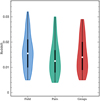 |
Fig. 1. Violin plot of the redshift distributions of our sample of late-type galaxies. The box plot inside each violin shows the interquartile range. The inner dot in the box plot represents the median of the distribution. The widths of the violin plots are scaled by the number of observations in each bin: 96 field galaxies, 64 galaxies in pairs, and 67 galaxies in groups. Only galaxies with maps of sSFR are shown. |
4. Results
In this work we study the effects of external and internal mechanisms on the radial distribution of the sSFR for late-type galaxies. To analyze the internal processes, we investigate the sSFR profiles of late-type galaxies split into bins of stellar mass. To investigate the external quenching effects, we compare late-type galaxies in three discrete environments: field galaxies, galaxies in pairs, and galaxies in groups. Our sample includes all CALIFA late-type galaxies with COMBO setup, for which we were able to construct sSFR maps.
Figure 2 shows the stellar mass distribution of late-type galaxies as a function of the environment. Median values (inner white dots inside the violin plots) are log(M⋆/M⊙) = 10.65, 10.49 and 10.66 for groups, pairs, and field galaxies, respectively.
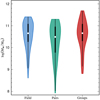 |
Fig. 2. Violin plot of the stellar mass for late-type galaxies as a function of the environment, as in Fig. 1. |
We split galaxies into four stellar mass bins: log(M⋆/M⊙) = 9.0−10.0, 10.0−10.5, 10.5−11.0 and 11.0−12.0. We have re-scaled each radial profile in terms of the r-band half-light effective radius, re, which has been computed following Graham et al. (2005) by using the SDSS r-band radius that encloses half the Petrosian flux and the concentration parameter in the same band. We consider the range 0–2.5 re to stack the radial profiles into eight bins, and we calculate the median value of r/re for each interval of size. Figure 3 shows examples of sSFR radial profiles, ΣsSFR, for galaxies in our sample. We show the median radial profiles for galaxies in the mass bin log(M*/M⊙) = 10.5−11.0: field galaxies (left panel), galaxies in pairs (central panel), and galaxies in groups (right panel). Profiles of individual galaxies are shown in gray, with the median profile for each bin in light blue. The shaded regions represent the 25% and 75% percentiles. Vertical error-bars were computed using the bootstrap re-sampling technique. Analogously to González Delgado et al. (2016), we have considered only mass bins containing more than five galaxies. We quote in all cases the number of galaxies contributing to each profile.
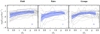 |
Fig. 3. An example of our stacking procedure: the stacked sSFR profiles, ΣsSFR, for late-type galaxies in the stellar mass range log(M⋆/M⊙) = 10.5−11.0 in field galaxies (left panel), galaxies in pairs (central panel), and galaxies in groups (right panel). Radial distances are normalized to the half-light effective radius re. Lines represent the median in each radial bin, and the shaded region shows the 25% and 75% percentiles. Vertical bars are the error in the median, and were computed by the bootstrap resampling technique. Individual profiles are shown by gray lines. |
Figure 4 compares the medians of ΣsSFR as a function of mass for each environment. In general, we observe two trends of ΣsSFR with increasing stellar mass: on the one hand, there is a global sSFR decrease, and on the other, there is a stronger drop towards the central regions. Profiles are nearly flat for galaxies with stellar masses below ∼1010 M⊙. For more massive galaxies, the central suppression of the sSFR strengthens with increasing mass. This behavior is observed independently of the environment. Our results are in agreement with Catalán-Torrecilla et al. (2017), Belfiore et al. (2018), and Spindler et al. (2018) in the sense that they found flat sSFR profiles for low-mass galaxies, and a significant decrease in the central regions of massive galaxies. This is consistent with the inside-out growth scenario or larger bulges.
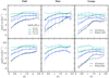 |
Fig. 4. The median profile of the sSFR, ΣsSFR, for late-type galaxies for different mass bins as a function of the environment: field galaxies (left panels), galaxies in pairs (central panels), and galaxies in groups (right panels). Solid lines represent the median in each radial bin. Vertical error bars were computed using the bootstrap re-sampling technique. The number of galaxies contributing to each median profile is quoted. Dashed lines in the upper (lower) panels show the median ΣsSFR profiles of spirals galaxies without AGNs (bars). For clarity, we excluded the vertical error bars in these profiles. |
There are several authors that support the inside-out mode in late-type galaxies (e.g., Muñoz Mateos et al. 2007, 2011; Pérez et al. 2013; Pezzulli et al. 2015; Ibarra-Medel et al. 2016). Alternatively, Abramson et al. (2014) argue in favor of an increase in bulge mass as a result of the suppression in the SFR, and Belfiore et al. (2018) argue that the sSFR suppression is not simply due to the larger mass of the bulge, but also the innate evolution of the sSFR in the context of inside-out growth. In addition, Spindler et al. (2018) find that at all masses, AGN/LINER galaxies are more likely to have centrally suppressed sSFR profiles than galaxies without AGN feedback.
We explore whether AGN feedback is the main mechanism responsible for the sSFR suppression in the inner regions of late-type galaxies. We recompute the ΣsSFR radial profile of late-type galaxies excluding AGNs. This is also seen in the upper panels of Fig. 4, as dashed lines. For the sake of clarity, we exclude the vertical error bars for the sample without AGNs. In general, we do not find significant differences in the median values of the sSFR profiles with or without AGNs. The frequencies of AGNs in the three environments are: 16%, 22%, and 35%, for field, pair, and group galaxies, respectively. To check whether the minor differences seen in Fig. 4 are indicative of actual differences between the populations, we rely on the test used by Muriel & Coenda (2014) and Martínez et al. (2016). Applied to our problem, this test computes the cumulative differences between two samples in the sSFR along the radial domain, and then checks whether the resulting quantity is consistent with the null hypothesis in which the two samples are drawn from the same underlying population in regards to their sSFR profiles. Results of the test are quoted in Table 2. In general, the null hypothesis in which the samples including or excluding AGNs are indistinguishable cannot be ruled out with a high level of confidence, highlighting the role played by AGNs secondary to the central role of stellar mass. Probable exceptions may be the third mass bin of field galaxies and of galaxies in pairs, for which the largest rejection levels are reached: 87% and 83%, respectively.
Probability of rejection of the null hypothesis in which the different subsamples are drawn from the same underlying distribution: comparison at fixed environment and mass bin.
Another factor that can play an important role in shaping the sSFR profiles is the presence of bars. Bars can trigger star formation in the central regions of galaxies. Several studies have found evidence of enhanced star formation activity in barred galaxies compared to those without bars (e.g., Heckman 1980; Regan et al. 2006; Lin et al. 2017). On the other hand, several other works in the literature do not find such differences (e.g., Pompea & Rieke 1990; Chapelon et al. 1999; Willett et al. 2015). Furthermore, Kim et al. (2017) found evidence that the star formation activity of strongly barred galaxies is on average lower than that of galaxies without bars. Barred galaxies amount to 34%, 36%, and 43%, in our field, pairs, and group samples, respectively. Similar to what we have done with AGNs, we recompute the ΣsSFR radial profile of late-type galaxies but now excluding barred galaxies. We show the resulting median profiles in the bottom panels of Fig. 4. We exclude the highest mass bin of galaxies in pairs, since there remained less than five galaxies in this bin once we had removed the barred ones. In general, the effect of bars in the radial profile of sSFR is negligible in our samples. The exception is the highest mass bin of galaxies in groups, where bars appear to enhance the sSFR of these galaxies at all scales, but more notably outside their half-light radii. The corresponding values of the rejection probability of the null hypothesis in which the samples including/excluding barred galaxies are drawn from the same population are also quoted in Table 2. These rejection probability values discard bars as an important factor shaping the sSFR profiles in late-type galaxies, with the exception of the highest mass bin in groups, for which the null hypothesis is rejected at a 91% level.
At this point we explore whether morphology can be an explanation for the suppression of star formation seen in Fig. 4, in the form of a dominant spheroidal component in the highest stellar mass bin. In Fig. 5 we show the distributions of the Hubble types of our sample of late-type galaxies, as a function of stellar mass and environment. For the two lowest stellar mass bins (top panels), we observe a mix of Hubble types. As stellar mass increases, we observe a higher fraction of Sa and Sb galaxies (bottom panels). However, there is no significant environmental dependence of the morphological type mix. The mass dependence of the sSFR profiles reflects the mass dependence mix of morphologies.
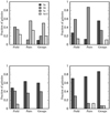 |
Fig. 5. Comparison of the distribution of the Hubble types for our sample of late-type galaxies, as a function of the environment. From top-left to bottom-right panel: log(M⋆/M⊙) = 9.0−10.0, 10.0−10.5, 10.5−11.0 and 11.0−12.0. |
In Fig. 6 we show the same radial profiles shown in Fig. 4 but comparing galaxies of the same mass across the three environments. As an overall trend, at fixed stellar mass, galaxies in groups are more suppressed at all radii than galaxies in pairs and in the field, with the exception of the inner regions (r/re ≲ 1) of galaxies in the lowest mass bin where there is no difference between environments. In general, galaxies in pairs show radial profiles that are intermediate between field and group galaxies, although their error bars are the largest given their small numbers. At the lowest mass bin, galaxies in groups show interesting features. Their sSFR profile is consistent with that of field galaxies up to r/re ∼ 1. This contrasts with the remaining mass bins where group galaxies show consistently lower sSFR values at all radii. On the other hand, at larger radii, r/re > 1, their star formation efficiency decays while field galaxies exhibit a flat behavior. At the other extreme in mass, the largest differences between the three environments are seen, with group galaxies having the steepest profile in the inner regions. For the two intermediate-mass bins, group and field galaxies have near parallel ΣsSFR profiles. The (very) small sample sizes prevent us from drawing strong conclusions from galaxies in pairs besides their sSFR intermediate between those of field and group galaxies. It is also worth mentioning that 87% of our galaxies in pairs are the brightest member of their pair. Our results do not change if we exclude those galaxies that are not the brightest member of their pair. In Table 3 we show the results of the test used above, now comparing the three environments at fixed mass bin. For all mass bins, the highest levels of rejection (95% level or higher) are reached in the comparison between field and group galaxies.
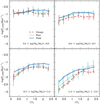 |
Fig. 6. Stacked profile of the sSFR ΣsSFR for late-type galaxies as a function of the environment. Each panel corresponds to a different mass bin. Galaxies in groups are shown in red lines, galaxies in pairs in green lines, and field galaxies in blue lines. Lines represent the median in each radial bin. Vertical error bars are as in Fig. 4. Field galaxies and galaxies in pairs have been shifted by 0.03 and −0.03 on the x-axis, respectively. |
The main difference between groups and the other environments explored here is an overall decrement of the sSFR. This decrement appears to be independent of the spatial scale at least for 10 ≤ log(M⋆/M⊙) ≤ 11. This fact could suggest that strangulation (e.g., Larson et al. 1980; Kawata & Mulchaey 2008; Peng et al. 2015) is the main mechanism responsible for the observed overall decrement in star formation, since it is proposed to produce a uniform suppression across the galaxy (van den Bergh 1991; Elmegreen et al. 2002). However, our sample may not cover the outermost parts of galaxies, where distinctive traces of such mechanisms may be clearer.
The differences seen in the lowest mass bin of Fig. 6, where we find an indication that the sSFR profile of group galaxies differs from that of field galaxies in a particular way, may be an indication of the effective action over these galaxies of mechanisms that act in an outside-in mode. Ram pressure stripping (Gunn & Gott 1972; Abadi et al. 1999; Book & Benson 2010; Steinhauser et al. 2016) could produce such a decrease of star formation in the outer parts of the disk, and a concentration of star formation in the inner parts (Rasmussen et al. 2006; Koopmann & Kenney 2004a,b; Cortese et al. 2011), thus providing an explanation for the observed profile. An alternative scenario could exist where tidal interactions produce central enhancements of star formation (e.g., Moreno et al. 2015) in galaxies where global star formation is otherwise suppressed by other precesses such as strangulation. Using numerical simulations, Yozin & Bekki (2015) found that the star formation in galaxies in groups may be influenced by both tidal interactions leading to central enhancement of star formation and ram pressure stripping inhibiting the SFR at large radii.
On the other hand, the main differences regarding the suppression in the inner regions of late-type galaxies are observed only for galaxies more massive than log(M⋆/M⊙) = 11, where the drop becomes stronger moving from field to group galaxies. Consistently with this, Welikala et al. (2008) found that local environment tends to reduce the SFR in central regions of galaxies. A distinct merger history of galaxies could explain the stronger drop seen in the inner regions of massive late types in groups (bottom-right panel of Fig. 6); a higher frequency of mergers in the past (e.g., Zandivarez et al. 2006; Zandivarez & Martínez 2011) may have caused the bulges of massive group spirals to shut down their star formation more effectively than in pairs and in the field.
Our results are in agreement with Schaefer et al. (2017), although they argue that environmental quenching occurs in an outside-in mode. It is worth noting that the sample of these latter authors includes galaxies of lower mass than ours, and it is at our lowest mass bin that we find evidence of outside-in environmental effects. Another difference with this work is that our sample extends further at the high-mass end. On the other hand, Spindler et al. (2018) did not find a correlation between local environment density and the profiles of the SFR surface density. One key difference between both of these works and ours, is that here we consider discrete environments instead of a continuously parametrized measure of the environment.
5. Summary
In this paper we analyze the dependence of the radial profiles of sSFR on environment and stellar mass, using a sample of late-type galaxies drawn from the CALIFA survey. We consider three different discrete environments: field galaxies, galaxies in pairs, and galaxies in groups. We split our galaxy samples into four bins of stellar mass, covering the range 9 ≤ log(M⋆/M⊙) ≤ 12, and compare their sSFR as a function of radius (in units of their effective radius) throughout the three environments. We note the following findings:
As in previous works in the literature, when we move from less to more massive galaxies, profiles of sSFR lower and bend towards the inner regions of the galaxies. Mass primarily determines the sSFR profiles of late-type galaxies.
Morphology matters: the relative size of the bulge plays a key role in depressing star formation towards the center of late-type galaxies.
The influence of AGNs and bars is secondary to mass.
The group environment determines clear differences in the sSFR profiles of galaxies. On the other hand, galaxies in pairs show sSFR that is intermediate between that of field and group galaxies.
There is evidence of an outside-in action upon galaxies with stellar masses 9 ≤ log(M⋆/M⊙) ≤ 10 in groups.
There is evidence of a much stronger star formation suppression in the inner regions of massive galaxies in groups, which may be an indication of a different merger history.
To distinguish whether the flat sSFR profiles seen for low-mass late-type galaxies in groups are the result of ram-pressure stripping that decreases star formation in the outer parts of disks, or are due to tidal interactions that enhance central star formation, a careful analysis of the age of the stellar populations as a function of radius may provide further clues. In a forthcoming paper (Coenda et al., in prep.) we focus on age profiles and explore the differences among the different environments.
Available as ancillary data tables at http://www.caha.es/CALIFA/public_html/?q=content/dr3-tables
Python CALIFA Starlight Synthesis organizer, http://pycasso.iaa.es
The NASA/IPAC Extragalactic Database (NED) is operated by the Jet Propulsion Laboratory, California Institute of Technology, under contract with the National Aeronautics and Space Administration, https://ned.ipac.caltech.edu/
Acknowledgments
This paper is based on data obtained by the CALIFA survey (http://califa.caha.es) which is based on observations collected at the Centro Astronómico Hispano Alemán (CAHA) at Calar Alto, operated jointly by the Max-Planck-Institut für Astronomie and the Instituto de Astrofísica de Andalucía (CSIC). This research has made use of the NASA/IPAC Extragalactic Database (NED), which is operated by the Jet Propulsion Laboratory, California Institute of Technology, under contract with the National Aeronautics and Space Administration. This paper has been partially supported with grants from Consejo Nacional de Investigaciones Científicas y Técnicas (PIP 11220130100365CO) Argentina, Fondo para la Investigación Científica y Tecnológica (FonCyT, PICT-2017-3301), and Secretaría de Ciencia y Tecnología, Universidad Nacional de Córdoba, Argentina.
References
- Abadi, M. G., Moore, B., & Bower, R. G. 1999, MNRAS, 308, 947 [NASA ADS] [CrossRef] [Google Scholar]
- Abazajian, K. N., Adelman-McCarthy, J. K., Agüeros, M. A., et al. 2009, ApJS, 182, 543 [NASA ADS] [CrossRef] [Google Scholar]
- Abramson, L. E., Kelson, D. D., Dressler, A., et al. 2014, ApJ, 785, L36 [NASA ADS] [CrossRef] [Google Scholar]
- Alam, S., Albareti, F. D., Allende Prieto, C., et al. 2015, ApJS, 219, 12 [NASA ADS] [CrossRef] [Google Scholar]
- Alpaslan, M., Driver, S., Robotham, A. S. G., et al. 2015, MNRAS, 451, 3249 [NASA ADS] [CrossRef] [Google Scholar]
- Asari, N. V., Cid Fernandes, R., Stasińska, G., et al. 2007, MNRAS, 381, 263 [NASA ADS] [CrossRef] [MathSciNet] [Google Scholar]
- Belfiore, F., Maiolino, R., Bundy, K., et al. 2018, MNRAS, 477, 3014 [NASA ADS] [CrossRef] [Google Scholar]
- Blanton, M. R., Bershady, M. A., Abolfathi, B., et al. 2017, AJ, 154, 28 [NASA ADS] [CrossRef] [Google Scholar]
- Book, L. G., & Benson, A. J. 2010, ApJ, 716, 810 [NASA ADS] [CrossRef] [Google Scholar]
- Bower, R. G., Benson, A. J., & Crain, R. A. 2012, MNRAS, 422, 2816 [NASA ADS] [CrossRef] [Google Scholar]
- Brough, S., Croom, S., Sharp, R., et al. 2013, MNRAS, 435, 2903 [NASA ADS] [CrossRef] [Google Scholar]
- Bryant, J. J., Owers, M. S., Robotham, A. S. G., et al. 2015, MNRAS, 447, 2857 [NASA ADS] [CrossRef] [Google Scholar]
- Bundy, K., Bershady, M. A., Law, D. R., et al. 2015, ApJ, 798, 7 [NASA ADS] [CrossRef] [Google Scholar]
- Cappellari, M., Emsellem, E., Krajnović, D., et al. 2011, MNRAS, 413, 813 [NASA ADS] [CrossRef] [Google Scholar]
- Catalán-Torrecilla, C., de Gil Paz, A., Castillo-Morales, A., et al. 2017, ApJ, 848, 87 [NASA ADS] [CrossRef] [Google Scholar]
- Chapelon, S., Contini, T., & Davoust, E. 1999, A&A, 345, 81 [NASA ADS] [Google Scholar]
- Cid Fernandes, R., Mateus, A., Sodré, L., Stasińska, G., & Gomes, J. M. 2005, MNRAS, 358, 363 [NASA ADS] [CrossRef] [Google Scholar]
- Cid Fernandes, R., Stasińska, G., Mateus, A., & Vale Asari, N. 2011, MNRAS, 413, 1687 [NASA ADS] [CrossRef] [Google Scholar]
- Cid Fernandes, R., Pérez, E., García Benito, R., et al. 2013, A&A, 557, A86 [NASA ADS] [CrossRef] [EDP Sciences] [Google Scholar]
- Cid Fernandes, R., Lacerda, E. A. D., González Delgado, R. M., et al. 2015, in Galaxies in 3D Across the Universe, ed. B. L. Ziegler, F. Combes, H. Dannerbauer, & M. Verdugo, IAU Symp., 309, 93 [NASA ADS] [Google Scholar]
- Cimatti, A., Brusa, M., Talia, M., et al. 2013, ApJ, 779, L13 [NASA ADS] [CrossRef] [Google Scholar]
- Cortese, L., Catinella, B., Boissier, S., Boselli, A., & Heinis, S. 2011, MNRAS, 415, 1797 [NASA ADS] [CrossRef] [Google Scholar]
- Dalla Vecchia, C., & Schaye, J. 2008, MNRAS, 387, 1431 [NASA ADS] [CrossRef] [Google Scholar]
- Darvish, B., Mobasher, B., Sobral, D., Scoville, N., & Aragon-Calvo, M. 2015, ApJ, 805, 121 [NASA ADS] [CrossRef] [Google Scholar]
- Darvish, B., Mobasher, B., Sobral, D., et al. 2016, ApJ, 825, 113 [NASA ADS] [CrossRef] [Google Scholar]
- de Amorim, A. L., García-Benito, R., Cid Fernandes, R., et al. 2017, MNRAS, 471, 3727 [NASA ADS] [CrossRef] [Google Scholar]
- Di Matteo, T., Springel, V., & Hernquist, L. 2005, Nature, 433, 604 [NASA ADS] [CrossRef] [PubMed] [Google Scholar]
- Elmegreen, D. M., Elmegreen, B. G., Frogel, J. A., et al. 2002, AJ, 124, 777 [NASA ADS] [CrossRef] [Google Scholar]
- García-Benito, R., Zibetti, S., Sánchez, S. F., et al. 2015, A&A, 576, A135 [NASA ADS] [CrossRef] [EDP Sciences] [Google Scholar]
- Girardi, M., Biviano, A., Giuricin, G., Mardirossian, F., & Mezzetti, M. 1993, ApJ, 404, 38 [NASA ADS] [CrossRef] [Google Scholar]
- Girardi, L., Bressan, A., Bertelli, G., & Chiosi, C. 2000, A&AS, 141, 371 [NASA ADS] [CrossRef] [EDP Sciences] [Google Scholar]
- González Delgado, R. M., Cerviño, M., Martins, L. P., Leitherer, C., & Hauschildt, P. H. 2005, MNRAS, 357, 945 [NASA ADS] [CrossRef] [Google Scholar]
- González Delgado, R. M., Cid Fernandes, R., Pérez, E., et al. 2016, A&A, 590, A44 [NASA ADS] [CrossRef] [EDP Sciences] [Google Scholar]
- Graham, A. W., Driver, S. P., Petrosian, V., et al. 2005, AJ, 130, 1535 [NASA ADS] [CrossRef] [Google Scholar]
- Gunn, J. E., & Gott, J. R. I. 1972, ApJ, 176, 1 [NASA ADS] [CrossRef] [Google Scholar]
- Guo, Q., White, S., Li, C., & Boylan-Kolchin, M. 2010, MNRAS, 404, 1111 [NASA ADS] [Google Scholar]
- Hasinger, G. 2008, A&A, 490, 905 [NASA ADS] [CrossRef] [EDP Sciences] [Google Scholar]
- Heckman, T. M. 1980, A&A, 88, 365 [NASA ADS] [Google Scholar]
- Hess, K. M., & Wilcots, E. M. 2013, AJ, 146, 124 [NASA ADS] [CrossRef] [Google Scholar]
- Hopkins, P. F., Quataert, E., & Murray, N. 2012, MNRAS, 421, 3522 [Google Scholar]
- Huchra, J. P., & Geller, M. J. 1982, ApJ, 257, 423 [NASA ADS] [CrossRef] [Google Scholar]
- Husemann, B., Jahnke, K., Sánchez, S. F., et al. 2013, A&A, 549, A87 [NASA ADS] [CrossRef] [EDP Sciences] [Google Scholar]
- Ibarra-Medel, H. J., Sánchez, S. F., Avila-Reese, V., et al. 2016, MNRAS, 463, 2799 [NASA ADS] [CrossRef] [Google Scholar]
- Jaffé, Y. L., Poggianti, B. M., Verheijen, M. A. W., Deshev, B. Z., & van Gorkom, J. H. 2012, ApJ, 756, L28 [NASA ADS] [CrossRef] [Google Scholar]
- Jedrzejewski, R. I. 1987, MNRAS, 226, 747 [Google Scholar]
- Kawata, D., & Mulchaey, J. S. 2008, ApJ, 672, L103 [Google Scholar]
- Kelz, A., Verheijen, M. A. W., Roth, M. M., et al. 2006, PASP, 118, 129 [NASA ADS] [CrossRef] [Google Scholar]
- Kenney, J. D. P., & Koopmann, R. A. 1999, AJ, 117, 181 [NASA ADS] [CrossRef] [Google Scholar]
- Kenney, J. D. P., Geha, M., Jáchym, P., et al. 2014, ApJ, 780, 119 [NASA ADS] [CrossRef] [Google Scholar]
- Khostovan, A. A., Sobral, D., Mobasher, B., et al. 2015, MNRAS, 452, 3948 [NASA ADS] [CrossRef] [Google Scholar]
- Kim, E., Hwang, H. S., Chung, H., et al. 2017, ApJ, 845, 93 [NASA ADS] [CrossRef] [Google Scholar]
- Koopmann, R. A., & Kenney, J. D. P. 2004a, ApJ, 613, 866 [NASA ADS] [CrossRef] [Google Scholar]
- Koopmann, R. A., & Kenney, J. D. P. 2004b, ApJ, 613, 851 [NASA ADS] [CrossRef] [Google Scholar]
- Larson, R. B., Tinsley, B. M., & Caldwell, C. N. 1980, ApJ, 237, 692 [NASA ADS] [CrossRef] [Google Scholar]
- Lin, L., Li, C., He, Y., Xiao, T., & Wang, E. 2017, ApJ, 838, 105 [NASA ADS] [CrossRef] [Google Scholar]
- Ludlow, A. D., Navarro, J. F., Angulo, R. E., et al. 2014, MNRAS, 441, 378 [NASA ADS] [CrossRef] [Google Scholar]
- Madau, P., Ferguson, H. C., Dickinson, M. E., et al. 1996, MNRAS, 283, 1388 [NASA ADS] [CrossRef] [Google Scholar]
- Marasco, A., Fraternali, F., & Binney, J. J. 2012, MNRAS, 419, 1107 [NASA ADS] [CrossRef] [Google Scholar]
- Martig, M., Bournaud, F., Teyssier, R., & Dekel, A. 2009, ApJ, 707, 250 [NASA ADS] [CrossRef] [Google Scholar]
- Martin, D. C., Fanson, J., Schiminovich, D., et al. 2005, ApJ, 619, L1 [Google Scholar]
- Martínez, H. J., Muriel, H., & Coenda, V. 2016, MNRAS, 455, 127 [NASA ADS] [CrossRef] [Google Scholar]
- Masters, K. L., Nichol, R. C., Hoyle, B., et al. 2011, MNRAS, 411, 2026 [NASA ADS] [CrossRef] [Google Scholar]
- McConnell, N. J., & Ma, C.-P. 2013, ApJ, 764, 184 [NASA ADS] [CrossRef] [Google Scholar]
- Merchán, M. E., & Zandivarez, A. 2005, ApJ, 630, 759 [NASA ADS] [CrossRef] [Google Scholar]
- Moore, B., Katz, N., Lake, G., Dressler, A., & Oemler, A. 1996, Nature, 379, 613 [NASA ADS] [CrossRef] [Google Scholar]
- Moore, B., Lake, G., Quinn, T., & Stadel, J. 1999, MNRAS, 304, 465 [NASA ADS] [CrossRef] [Google Scholar]
- Moreno, J., Torrey, P., Ellison, S. L., et al. 2015, MNRAS, 448, 1107 [NASA ADS] [CrossRef] [Google Scholar]
- Muñoz Mateos, J. C., Gil de Paz, A., Boissier, S., et al. 2007, ApJ, 658, 1006 [NASA ADS] [CrossRef] [Google Scholar]
- Muñoz Mateos, J. C., Boissier, S., de Gil Paz, A., et al. 2011, ApJ, 731, 10 [NASA ADS] [CrossRef] [Google Scholar]
- Muriel, H., & Coenda, V. 2014, A&A, 564, A85 [NASA ADS] [CrossRef] [EDP Sciences] [Google Scholar]
- Muzzin, A., Wilson, G., Yee, H. K. C., et al. 2012, ApJ, 746, 188 [NASA ADS] [CrossRef] [Google Scholar]
- Nandra, K., Georgakakis, A., Willmer, C. N. A., et al. 2007, ApJ, 660, L11 [NASA ADS] [CrossRef] [Google Scholar]
- Navarro, J. F., Frenk, C. S., & White, S. D. M. 1996, ApJ, 462, 563 [NASA ADS] [CrossRef] [Google Scholar]
- Peng, Y.-J., Lilly, S. J., Kovač, K., et al. 2010, ApJ, 721, 193 [NASA ADS] [CrossRef] [Google Scholar]
- Peng, Y., Maiolino, R., & Cochrane, R. 2015, Nature, 521, 192 [NASA ADS] [CrossRef] [Google Scholar]
- Pérez, E., Cid Fernandes, R., González Delgado, R. M., et al. 2013, ApJ, 764, L1 [NASA ADS] [CrossRef] [Google Scholar]
- Pezzulli, G., Fraternali, F., Boissier, S., & Muñoz-Mateos, J. C. 2015, MNRAS, 451, 2324 [NASA ADS] [CrossRef] [Google Scholar]
- Pompea, S. M., & Rieke, G. H. 1990, ApJ, 356, 416 [NASA ADS] [CrossRef] [Google Scholar]
- Rasmussen, J., Ponman, T. J., & Mulchaey, J. S. 2006, MNRAS, 370, 453 [NASA ADS] [CrossRef] [Google Scholar]
- Rasmussen, J., Ponman, T. J., Verdes-Montenegro, L., Yun, M. S., & Borthakur, S. 2008, MNRAS, 388, 1245 [NASA ADS] [CrossRef] [Google Scholar]
- Regan, M. W., Thornley, M. D., Vogel, S. N., et al. 2006, ApJ, 652, 1112 [NASA ADS] [CrossRef] [Google Scholar]
- Roth, M. M., Kelz, A., Fechner, T., et al. 2005, PASP, 117, 620 [NASA ADS] [CrossRef] [Google Scholar]
- Sales, L. V., Navarro, J. F., Abadi, M. G., & Steinmetz, M. 2007, MNRAS, 379, 1475 [NASA ADS] [CrossRef] [Google Scholar]
- Salpeter, E. E. 1955, ApJ, 121, 161 [Google Scholar]
- Sánchez, S. F., Kennicutt, R. C., de Gil Paz, A., et al. 2012, A&A, 538, A8 [NASA ADS] [CrossRef] [EDP Sciences] [Google Scholar]
- Sánchez, S. F., García-Benito, R., Zibetti, S., et al. 2016a, A&A, 594, A36 [NASA ADS] [CrossRef] [EDP Sciences] [Google Scholar]
- Sánchez, S. F., Pérez, E., Sánchez-Blázquez, P., et al. 2016b, Rev. Mex. Astron. Astrofis., 52, 171 [Google Scholar]
- Schaefer, A. L., Croom, S. M., Allen, J. T., et al. 2017, MNRAS, 464, 121 [NASA ADS] [CrossRef] [Google Scholar]
- Schaller, G., Schaerer, D., Meynet, G., & Maeder, A. 1992, A&AS, 96, 269 [Google Scholar]
- Silverman, J. D., Mainieri, V., Lehmer, B. D., et al. 2008, ApJ, 675, 1025 [NASA ADS] [CrossRef] [Google Scholar]
- Singh, R., van de Ven, G., Jahnke, K., et al. 2013, A&A, 558, A43 [NASA ADS] [CrossRef] [EDP Sciences] [Google Scholar]
- Smethurst, R. J., Lintott, C. J., Simmons, B. D., et al. 2015, MNRAS, 450, 435 [NASA ADS] [CrossRef] [Google Scholar]
- Sobral, D., Best, P. N., Smail, I., et al. 2011, MNRAS, 411, 675 [NASA ADS] [CrossRef] [Google Scholar]
- Sobral, D., Smail, I., Best, P. N., et al. 2013, MNRAS, 428, 1128 [NASA ADS] [CrossRef] [Google Scholar]
- Spindler, A., Wake, D., Belfiore, F., et al. 2018, MNRAS, 476, 580 [NASA ADS] [CrossRef] [Google Scholar]
- Steinhauser, D., Schindler, S., & Springel, V. 2016, A&A, 591, A51 [NASA ADS] [CrossRef] [EDP Sciences] [Google Scholar]
- Stringer, M. J., Bower, R. G., Cole, S., Frenk, C. S., & Theuns, T. 2012, MNRAS, 423, 1596 [NASA ADS] [CrossRef] [Google Scholar]
- van den Bergh, S. 1991, PASP, 103, 390 [NASA ADS] [CrossRef] [Google Scholar]
- Vazdekis, A., Sánchez-Blázquez, P., Falcón-Barroso, J., et al. 2010, MNRAS, 404, 1639 [NASA ADS] [Google Scholar]
- Verdes-Montenegro, L., Sulentic, J., Lisenfeld, U., et al. 2005, A&A, 436, 443 [NASA ADS] [CrossRef] [EDP Sciences] [Google Scholar]
- Walcher, C. J., Wisotzki, L., Bekeraité, S., et al. 2014, A&A, 569, A1 [NASA ADS] [CrossRef] [EDP Sciences] [Google Scholar]
- Welikala, N., Connolly, A. J., Hopkins, A. M., Scranton, R., & Conti, A. 2008, ApJ, 677, 970 [NASA ADS] [CrossRef] [Google Scholar]
- Willett, K. W., Schawinski, K., Simmons, B. D., et al. 2015, MNRAS, 449, 820 [NASA ADS] [CrossRef] [Google Scholar]
- Yoshida, M., Yagi, M., Komiyama, Y., et al. 2008, ApJ, 688, 918 [NASA ADS] [CrossRef] [Google Scholar]
- Yozin, C., & Bekki, K. 2015, MNRAS, 453, 14 [NASA ADS] [CrossRef] [Google Scholar]
- Zandivarez, A., & Martínez, H. J. 2011, MNRAS, 415, 2553 [NASA ADS] [CrossRef] [Google Scholar]
- Zandivarez, A., Martínez, H. J., & Merchán, M. E. 2006, ApJ, 650, 137 [NASA ADS] [CrossRef] [Google Scholar]
All Tables
Probability of rejection of the null hypothesis in which the different subsamples are drawn from the same underlying distribution: comparison at fixed environment and mass bin.
All Figures
|
Fig. 1. Violin plot of the redshift distributions of our sample of late-type galaxies. The box plot inside each violin shows the interquartile range. The inner dot in the box plot represents the median of the distribution. The widths of the violin plots are scaled by the number of observations in each bin: 96 field galaxies, 64 galaxies in pairs, and 67 galaxies in groups. Only galaxies with maps of sSFR are shown. |
| In the text | |
|
Fig. 2. Violin plot of the stellar mass for late-type galaxies as a function of the environment, as in Fig. 1. |
| In the text | |
|
Fig. 3. An example of our stacking procedure: the stacked sSFR profiles, ΣsSFR, for late-type galaxies in the stellar mass range log(M⋆/M⊙) = 10.5−11.0 in field galaxies (left panel), galaxies in pairs (central panel), and galaxies in groups (right panel). Radial distances are normalized to the half-light effective radius re. Lines represent the median in each radial bin, and the shaded region shows the 25% and 75% percentiles. Vertical bars are the error in the median, and were computed by the bootstrap resampling technique. Individual profiles are shown by gray lines. |
| In the text | |
|
Fig. 4. The median profile of the sSFR, ΣsSFR, for late-type galaxies for different mass bins as a function of the environment: field galaxies (left panels), galaxies in pairs (central panels), and galaxies in groups (right panels). Solid lines represent the median in each radial bin. Vertical error bars were computed using the bootstrap re-sampling technique. The number of galaxies contributing to each median profile is quoted. Dashed lines in the upper (lower) panels show the median ΣsSFR profiles of spirals galaxies without AGNs (bars). For clarity, we excluded the vertical error bars in these profiles. |
| In the text | |
|
Fig. 5. Comparison of the distribution of the Hubble types for our sample of late-type galaxies, as a function of the environment. From top-left to bottom-right panel: log(M⋆/M⊙) = 9.0−10.0, 10.0−10.5, 10.5−11.0 and 11.0−12.0. |
| In the text | |
|
Fig. 6. Stacked profile of the sSFR ΣsSFR for late-type galaxies as a function of the environment. Each panel corresponds to a different mass bin. Galaxies in groups are shown in red lines, galaxies in pairs in green lines, and field galaxies in blue lines. Lines represent the median in each radial bin. Vertical error bars are as in Fig. 4. Field galaxies and galaxies in pairs have been shifted by 0.03 and −0.03 on the x-axis, respectively. |
| In the text | |
Current usage metrics show cumulative count of Article Views (full-text article views including HTML views, PDF and ePub downloads, according to the available data) and Abstracts Views on Vision4Press platform.
Data correspond to usage on the plateform after 2015. The current usage metrics is available 48-96 hours after online publication and is updated daily on week days.
Initial download of the metrics may take a while.