| Issue |
A&A
Volume 621, January 2019
|
|
|---|---|---|
| Article Number | A60 | |
| Number of page(s) | 14 | |
| Section | Catalogs and data | |
| DOI | https://doi.org/10.1051/0004-6361/201833956 | |
| Published online | 08 January 2019 | |
Near-infrared spectroscopic indices for unresolved stellar populations
I. Template galaxy spectra⋆,⋆⋆
1
GEPI, Observatoire de Paris, PSL Research University, CNRS, Univ. Paris Diderot, Sorbonne Paris Cité, 61 Avenue de l’Observatoire, 75014 Paris, France
e-mail: This email address is being protected from spambots. You need JavaScript enabled to view it.
2
Instituto de Astronomìa y Ciencias Planetarias Universidad de Atacama, Copiapò, Chile
3
Dipartimento di Fisica e Astronomia “G. Galilei”, Università di Padova, Vicolo dell’Osservatorio 3, 35122 Padova, Italy
4
INAF-Osservatorio Astronomico di Padova, Vicolo dell’Osservatorio 5, 35122
Padova, Italy
5
European Southern Observatory, Karl-Schwarzschild-Str. 2, 85748
Garching bei München, Germany
6
European Southern Observatory, Ave. Alonso de Córdova 3107, Vitacura, Santiago, Chile
Received:
26
July
2018
Accepted:
8
October
2018
Abstract
Context. A new generation of spectral synthesis models has been developed in recent years, but there is no matching set of template galaxy spectra, in terms of quality and resolution, for testing and refining the new models.
Aims. Our main goal is to find and calibrate new near-infrared spectral indices along the Hubble sequence of galaxies which will be used to obtain additional constraints to the population analysis based on medium-resolution integrated spectra of galaxies.
Methods. Spectra of previously studied and well-understood galaxies with relatively simple stellar populations (e.g., ellipticals or bulge dominated galaxies) are needed to provide a baseline data set for spectral synthesis models.
Results. X-shooter spectra spanning the optical and infrared wavelengths (350–2400 nm) of bright nearby elliptical galaxies with a resolving power of R ∼ 4000–5400 were obtained. Heliocentric systemic velocity, velocity dispersion, and Mg, Fe, and Hβ line-strength indices are presented.
Conclusions. We present a library of very-high-quality spectra of galaxies covering a large range of age, metallicity, and morphological type. Such a dataset of spectra will be crucial to addressing important questions of the modern investigation concerning galaxy formation and evolution.
Key words: surveys / infrared: galaxies / galaxies: abundances / galaxies: stellar content / galaxies: formation
Based on observations made with ESO Telescopes at the La Silla Paranal Observatory under programme ID 086.B-0900(A).
The reduced spectra (FITS files) are only available at the CDS via anonymous ftp to cdsarc.u-strasbg.fr (130.79.128.5) or via http://cdsarc.u-strasbg.fr/viz-bin/qcat?J/A+A/621/A60
© ESO 2019
1. Introduction
Recent advances in the infrared (IR) instruments like X-shooter Vernet et al. (2011) and KMOS (Sharples et al. 2013) and their availability at the large telescopes have made it possible to extend the stellar population studies of unresolved galaxies into the IR domain (see e.g., the pioneering work of Rieke et al. 1980, 1988). Reduction of the extinction is obviously beneficial, but is not the only advantage of the expansion towards longer wavelengths; a look at the color-magnitude diagram of any complex stellar system suggests that different stellar populations dominate different spectral ranges (see the discussion in Riffel et al. 2011a; Mason et al. 2015), opening up the possibility to disentangle their contribution in these systems.
Comprehensive stellar libraries are the first step toward developing the necessary tools for IR studies. An incomplete list of the previous work includes Johnson & Méndez (1970), Kleinmann & Hall (1986), Lambert et al. (1986), Origlia et al. (1993), Wallace & Hinkle (1997, 2002), Joyce et al. (1998), Meyer et al. (1998), Wallace et al. (2000), Ivanov et al. (2004), and Zamora et al. (2015); for more historic references see Table 1 in Rayner et al. (2009). The early theoretical attempts to model the IR stellar spectra faced difficulties with the incorporation of millions of molecular lines, and generated synthetic spectra that did not match well the broad band features due to complications with the broad molecular features (Castelli et al. 1997). Late-type stars with prominent molecular bands were sometimes omitted, even for optical spectral models (Buser & Kurucz 1992).
These observational libraries quickly found other applications to derive stellar diagnostics in heavily obscured regions (Tamblyn et al. 1996; Hanson et al. 1997, 2002; Messineo et al. 2009) and for objects that are intrinsically bright in the IR because of their low effective temperatures; such as brown dwarfs, (Oppenheimer et al. 1995; Geballe et al. 1996; Gorlova et al. 2003; Bonnefoy et al. 2014) asymptotic giant branch (AGB), red giant, and red supergiant stars (Lambert et al. 1986; Terndrup et al. 1991; Ramirez et al. 1997; Lançon & Wood 2000; Davies et al. 2013).
A major step in the development of libraries came with the work of Rayner et al. (2009, i.e., the IRTF spectral library).
This latter library includes 210 stars, observed at a resolving power of R ∼ 2000, and has a spectral coverage from λ ∼ 0.8 μm to 2.5 μm. An earlier precursor paper (Cushing et al. 2005) included spectra of ultracool M, L, and T-type dwarfs observed with the same instrument setup. This was the first flux-calibrated IR stellar library which facilitated its use for modeling the integral spectra of galaxies.
The first generation of evolutionary models with a proper treatment of the IR wavelength range (Maraston 2005) used theoretical stellar spectra (Lejeune et al. 1997, 1998) but the availability of the empirical IRTF spectral library prompted the development of a number of models based on it. Conroy & van Dokkum (2012) pointed at the presence of features sensitive to the initial mass function (IMF) slope – age and [α/Fe]abundance ratio. Meneses-Goytia et al. (2015a) carried out extensive preparation of the IRTF library and reported, in a companion paper (Meneses-Goytia et al. 2015b), a new synthetic model that fitted well the published indices of elliptical galaxies. Röck et al. (2015) from the same research group extended the population models from λ ∼ 2.5 μm to 5 μm with the subset of the IRTF library spectra that covered this wavelength range. These models agree well with the observations for older galaxies, but have problems with younger and/or metal-poor populations. Finally, a combined model spanning the entire optical-IR range was reported in Röck et al. (2016), together with new tests that further validate its results.
This progress revealed an unexpected problem – the lack of matching high-quality galaxy spectra. An example of a forced “work around” resorting to broad band photometry for population synthesis purposes is the work of Coelho et al. (2005), but there are also on-going efforts to obtain IR spectra of galaxies. Not surprisingly, the first of these were aimed at the classes of obscured objects for which these challenging observations yielded the biggest advantages: star-forming galaxies (Rieke et al. 1988; Doyon et al. 1994a,b; Engelbracht et al. 1998; Vanzi et al. 1996; Vanzi & Rieke 1997; Kotilainen et al. 2001), luminous and ultra-luminous IR galaxies (LIRG and ULIRG; Doyon et al. 1994a; Veilleux et al. 1997a, 1999), and galaxies with active nuclei (AGNs; Veilleux et al. 1997b; Ivanov et al. 2000; Reunanen et al. 2002, 2003; Imanishi & Alonso-Herrero 2004; Riffel et al. 2006; Hyvönen et al. 2009; Mould et al. 2012). The influx of more and better spectra of galaxies with various types of activity continues, but most of these studies lack the signal-to-noise ratio (S/N) needed to investigate the galaxy continuum and absorption features; instead, they concentrated on the emission lines and tried to address general questions regarding the nature of the hidden (in the optical wavelengths, at least) power sources and the contribution of the AGN – far from determining the parameters of the stellar populations directly from absorption features, as has been done in the optical for many years (e.g., Worthey 1994).
Encouragingly, Mason et al. (2015) found some differences in the strength of absorption features and the continuum shapes in galaxies with younger stellar populations – for example, Balmer absorption lines are associated with populations younger than 1.5 Gyr. They also found the behavior of some metal features to be promising, but their sample was dominated by low-ionization nuclear emission-line region (LINERS) and Seyferts and only in a few cases was the activity sufficiently low that it did not significantly affect the stellar continuum.
The contribution of the AGB stars to the total galaxy spectra is another open issue. Molecular CN and VO bands that originate in thermally pulsating AGB (TP-AGB) stars were also detected by Mason et al. (2015), but these features were weaker in ∼1 Gyr galaxies than in older ones. This may be a bias related to the intrinsic velocity dispersion and the contamination from other features. Zibetti et al. (2013) found TP-AGB stars in post-starburst galaxies with ages 0.5–1.5 Gyr to have a negligible contribution. More recently Riffel et al. (2015a) called for a revision of models of Maraston & Strömbäck (2011) to reduce the contribution of TP-AGB stars. On the other hand Mármol-Queraltó et al. (2009) measured systematically stronger K-band NaI and CO in galaxies with an AGB population than in those without one, and therefore the question of whether younger populations can be reliably detected with IR spectroscopy remains open.
At least one of our galaxies, NGC 7424 has an age estimate (Table 3) that suggests it may contain significant populations of AGB stars. The age estimates are luminosity weighted and the high intrinsic luminosity of the AGB stars in the IR range implies that these stars contribute a notable fraction to the total IR light of the galaxies (e.g., ∼17 % at H band; Melbourne et al. 2012).
The AGB stars are surrounded by dust envelopes that reprocess the stellar light and re-emit it to the near- or mid-IR, although to obtain a good fit to the observed near-/mid-IR spectral energy distribution of the galaxies may require adjustment of the AGB lifetimes (e.g., Villaume et al. 2015). The fast- and short-lived AGB phases lead to luminosity fluctuations that affect the M/L ratio (Lançon et al. 2000; Maraston et al. 2011), especially in the IR, and the star formation rate (SFR) estimates. The AGB stars are responsible for the dust production and therefore the intrinsic reddening inside galaxies. Furthermore, the intrinsically red AGB stars modify the apparent galaxy colors to appear redder at younger age; omitting the AGB contribution leads to incorrect age and mass estimates (Maraston et al. 2006).
All these effects increase with redshift, when progressively younger galaxies are observed. Therefore, better stellar population models that include the effects of the AGB stars will be needed to interpret the observations for the James Webb space telescope. These models are being prepared (e.g., Marigo et al. 2017) and our library is intended to help test and validate them.
Another basic question in studies of unresolved galaxies refers to the slope of the IMF. Constraining the IMF requires access to gravity-sensitive features and the IR region contains some of these: the CO bands (Ivanov et al. 2004) and the Na I doublet at 1.14 μm (Smith et al. 2015). Their behavior suffers from a degeneracy between the IMF slope and metallicity, and therefore a more complex approach to solving the stellar populations is needed here.
Finally, the IR absorption features allow us to probe the kinematics of different stellar populations – Riffel et al. (2015b) found that the IR velocity dispersion σIR is lower than the optical σopt and explained this result either with the presence of warm dust that filled in the CO bands, used to measure σIR, or with contribution from a redder, dynamically colder stellar population that dominates the IR light. Disentangling between these possibilities requires spatially resolved kinematic measurements, which are within the reach of the present state-of-the-art IR instrumentation.
The above questions have motivated efforts to obtain a large high-quality data set of “normal” and relatively simple stellar systems – both galaxies and star clusters – that can be used as relatively straightforward test cases to gain understanding of the behavior of IR spectral features and to test models. Lyubenova et al. (2010, 2012) and Riffel et al. (2011b) reported integrated spectra over entire star clusters, while Silva et al. (2008), Cesetti et al. (2009), Kotilainen et al. (2012), and Mason et al. (2015) provided spectra of quiescent galaxies.
Here we present new templates of galaxy spectra with a resolving power of R ∼ 4000, spanning a wavelength range from 0.3 to 2.4 μm. These were obtained with the X-shooter spectrograph at the European Southern Observatory Very Large telescope (ESO VLT), matching the most comprehensive recent stellar spectral library (still partially a work in progress; see Chen et al. 2014; Gonneau et al. 2016). We provide high-quality test data facilitating the understanding of the IR spectral diagnostic tools and the testing of the newest generation of spectral synthesis models. Our library spans a combined optical–NIR range obtained with the same instrument and sampling the same spatial region of the galaxies, unlike the previous libraries. Thus, we minimize any systematic error that may originate from sampling of the stellar population gradients inside the galaxies. Our sample is dominated by well-characterized objects with known and understood stellar populations, spanning a range of ages and metallicities. This is the first paper in a series; it describes the data obtained. Indices and other results will be reported in further publications.
2. Galaxy sample selection
The galaxies in the sample have been selected to be bright (Bt ∼ 11 − 13 mag) and distributed along the Hubble sequence from ellipticals to late-type spirals. We preferred early-type galaxies, because they generally represent simpler stellar populations than the spirals, and thus facilitate an easier testing of stellar population models. We gave further priority to objects with age and metallicity already available in the literature.
The basic properties of our sample of galaxies are reported in Table 1. Some literature data for our galaxies that were used for various comparisons throughout this paper are listed in Tables A.1–A.4. If possible, we gave preference to literature sources that have multiple objects in common with our sample.
Parameters of the sample galaxies.
3. Observations and data reduction
The data were acquired with the X-shooter (Guinouard et al. 2006), a spectrograph at the Unit 2 of ESO Very Large Telescope on Paranal (Chile). This is a three arms cross-dispersed spectrograph that provides continuous coverage over λ ∼ 360–2500 nm. We used 1.3, 1.5, and 1.2 arcsec wide slits for the ultraviolet (UBV), visual (VIS), and NIR arms, yielding average resolving power of about 4000, 5400, and 4300, respectively. The binning in the UBV and VIS arms was 1 × 1.
We observed the sample of galaxies along their major axis with the aim to also derive the values of the stellar population properties in the center of the galaxy and to evaluate their gradient along the major axis. In the final spectra even if the S/N was very high, it was not enough to measure the gradients of the stellar population properties in the NIR spectral region and we finally co-added the spectra along the spatial axis in order to increase the final S/N. This results in spectra mapping a region of about 1.5 × 1.5 arcsec around the center that covers an area between 65 and 430 pc.
For all the targets, multiple exposures have been acquired to better remove the detectors’ cosmetics. The NIR observations were further split to remove the sky emission and avoid saturation of the brightest sky lines. For most galaxies we sampled clear sky offsetting away from the target, except for a few more compact ones for which we observed in stare mode. A summary of the observations is presented in Table 2.
Observing log.
The spectra were reduced using the X-shooter pipeline version 2.6.8. (Goldoni et al. 2006) in the ESO Reflex workflow environment version 2.8.1 (Freudling et al. 2013). The basic processing steps are bias and background subtraction, cosmic ray removal (van Dokkum 2001), sky subtraction (Kelson 2003), flat-fielding, order extraction, and merging. The telluric corrections were performed with molecfit, a software tool designed to remove atmospheric absorption features from astronomical spectra (Smette et al. 2015).
The one-dimensional (1D) spectrum extraction was performed over a region of ±2″ from the peak value of the spectrum. A flux correction was applied to take into account the regions outside these limits by fitting a Gaussian profile to the cross order profile and integrating over the fit to obtain the total flux. The spectra from the three X-shooter arms were combined matching them to the bluest spectrum, so the UBV arm is anchoring the overall flux calibration.
The final products are shown in Figs. 1 and B.1. A flux-weighted combined spectrum with 3σ rejection is also plotted.
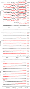 |
Fig. 1. Spectra of the sample galaxies in different wavelength ranges. Each spectrum is normalized to unity, shifted for displaying purposes, and labeled with the NGC number of the galaxy. The spectra at the top of each panel are the average of the sample spectra (see Sect. 3). |
4. Data-quality validation
First, to evaluate the internal consistency of the galaxy spectra we compared the products generated from different observations of the same galaxy (Fig. A.1). For example, the root mean square (rms) of the difference over intervals of 14–20 nm are ∼1.5% and 8–10% for NGC 1425 and NGC 4415, respectively. The resulting values reflect the different S/N of the spectra, while the flat residuals are an indication of the lack of systematic effects.
Next, a number of optical spectra of the galaxies in our sample are available from the literature (Table A.5). They provide an external check. Unfortunately, the largest overlap with eight objects in common with the 6dF survey (Jones et al. 2009) is not useful, because their spectra were obtained with a fiber spectrograph and are not flux calibrated (Fig. A.2). Comparisons with some flux-calibrated spectra from other sources are plotted in Fig. 2 and show reasonably good matches. The most notable deviations are in the overall slopes.
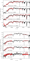 |
Fig. 2. Comparison between our optical spectra (black lines) with literature spectra (red lines) scaled to match the flux level of ours. Top panels: spectra of NGC 3379 from different sources as given in the labels. Bottom panels: spectra of the four galaxies in common with Ho et al. (1995). Their spectra consist of two portions, which we separately scaled to match our spectrum. |
Unfortunately, there is no overlap between our sample and those of the more modern NIR spectroscopic surveys of galaxies (e.g., Silva et al. 2008; Cesetti et al. 2009; Kotilainen et al. 2012; Mould et al. 2012; Mason et al. 2015). NGC 3379 was observed by Ivanov et al. (2000), but only in the K atmospheric window, and with low S/N ∼ 50 and a resolving power of only R ∼ 1200. Cesetti et al. (2009) published an average low-resolution (R ∼ 1000) NIR spectrum of elliptical galaxies. A direct comparison with the NIR spectra of five bonafide ellipticals show deviations of up to 15% over a single atmospheric window.
Following the example of other spectral libraries, we attempted to evaluate how well our data processing recovers the shape of the spectra. This issue is particularly important for data taken with cross-dispersed spectrographs, which implies that the final spectrum is assembled from multiple, essentially independently reduced spectral orders. Rayner et al. (2009) generated synthetic Two Micron All Sky Survey (2MASS; Skrutskie et al. 2006) colors for the stars in their sample and compared them with the actual 2MASS observations. However, this is only a straightforward test for stellar spectra where the slit size and the seeing have limited effect. Furthermore, galaxies may have radial stellar population gradients that could drive radial color gradients; therefore, it is important to match the apertures used for observing in different photometric band-passes both between themselves and between them and the slit apertures used to extract our spectra. X-shooter uses slits of different sizes for each of its three arms, but we matched the fluxes during the combination (see Sect. 3), and therefore the flux difference originating from the slit apertures cancels out to zero order; some residual effect related to the galaxy profiles and color gradients may remain.
A search through the literature identified no homogeneous multi-band and multi-galaxy flux measurements for our galaxies within apertures with sizes as small as a few arcseconds. One exception, and only in terms of using a uniform aperture to measure the apparent galaxy magnitudes in the same apertures, is the work of Brown et al. (2014). They report measurements for the Sloan Digital Sky Survey (SDSS; York et al. 2000) and the 2MASS sets of filters (Fukugita et al. 1996; Cohen et al. 2003) for two of our galaxies (NGC 584 and NGC 3379), although they use wide apertures: apertures of 18 × 55 arcsec2 and 180 × 120 arcsec2, respectively. To facilitate the comparison we formed the difference between the SDSS and 2MASS magnitudes derived from our spectra and their apparent magnitudes, and subtracted the median for each galaxy, effectively removing the aperture effects. The result is shown in Fig. 3. The rms is 0.16 mag for NGC 584 and 0.09 mag for NGC 3379, indicating a reasonably good agreement. Removing the two largest outliers – u and Ks – reduces these values to 0.08 mag and 0.05 mag, respectively, which is comparable to the quality of the stellar spectra of Brown et al. (2014).
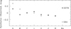 |
Fig. 3. Comparison between the synthetic apparent magnitudes derived from our spectra and observed apparent magnitudes reported by Brown et al. (2014) for NGC 584 (open circles) and NGC 3379 (solid dots). |
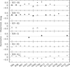 |
Fig. 4. A comparison of synthetic broad band colors generated from our spectra and apparent colors form the literature, listed in Table C.1. |
The apparent colors for the central 1.3 × 4 arcsec2 of the galaxies in our sample, derived from the X-shooter spectra, in some of the more commonly used photometric systems are listed Table C.1.
5. Stellar kinematics and line-strength indices
We measured the line-of-sight velocity distribution of the stellar component of the sample galaxies from the absorption lines in the observed wavelength range using the Penalized Pixel Fitting (PPXF; Cappellari & Emsellem 2004) and Gas and Absorption Line Fitting (GANDALF; Sarzi et al. 2006) with a code which we adapted to deal with X-shooter spectra. In addition, we simultaneously fitted the ionized-gas emission lines detected with a S/N > 3 and we derived the heliocentric radial velocity VH and velocity dispersion σV of the stars in the central region of galaxies. We give the measured stellar kinematics in Table 3.
Central values of the velocity, dispersion, line-strength indices, age, and metallicity of the sample galaxies measured within an aperture of radius 0.3 re.
We measured the most commonly used Mg, Fe, and Hβ line-strength indices of the Lick/IDS system (Faber et al. 1985); 1994ApJS...94..687W, the iron index 〈Fe〉 = (Fe5270+Fe5335)/2 of Gorgas et al. (1990), the combined magnesium-iron index ![Mathematical equation: $ [\mathrm{MgFe}]\prime=\sqrt{\mathrm{Mg}\,b\,(0.72\times \mathrm{Fe5270} + 0.28\times\mathrm{Fe5335})} $](/articles/aa/full_html/2019/01/aa33956-18/aa33956-18-eq3.gif) of Thomas et al. (2003) and their errors by following the same procedures as in Morelli et al. (2004, 2015, 2016). We calculated the central values of Mgb, Mg2, Hβ, ⟨Fe⟩, [MgFe]′ and the velocity dispersion σV, all within 0.3 re, where re is the effective radius of the galaxy. They are reported in Table 3. To verify our measurements we compared them with the literature data both directly and with the model-dependent abundance estimates [Z/H]. The plots show clear and well-defined trends. The most discrepant values come from NGC 3423, one of the two galaxies with the lowest S/N ratios. The rms of the direct comparison is: 18 km s−1 for σV, 0.14 Å for ⟨Fe⟩ and Mg2, and 0.22 mag for Mgb.
of Thomas et al. (2003) and their errors by following the same procedures as in Morelli et al. (2004, 2015, 2016). We calculated the central values of Mgb, Mg2, Hβ, ⟨Fe⟩, [MgFe]′ and the velocity dispersion σV, all within 0.3 re, where re is the effective radius of the galaxy. They are reported in Table 3. To verify our measurements we compared them with the literature data both directly and with the model-dependent abundance estimates [Z/H]. The plots show clear and well-defined trends. The most discrepant values come from NGC 3423, one of the two galaxies with the lowest S/N ratios. The rms of the direct comparison is: 18 km s−1 for σV, 0.14 Å for ⟨Fe⟩ and Mg2, and 0.22 mag for Mgb.
We derived the stellar population properties in the center of the sample galaxies by comparing the measurements of the line-strength indices with the model predictions by Johansson et al. (2010) for the single stellar population as a function of age and metallicity. We calculated the age and metallicity in the center of the sample galaxies from the central values of line-strength indices given in Table 3. The central values of Hβ and [MgFe]′ are compared with the model predictions by Johansson et al. (2010). In this parameter space the mean age and total metallicity appear to be almost insensitive to the variations of the α/Fe enhancement. The central mean age and total metallicity of the stellar population in the center of the sample galaxies were derived from the values of line-strength indices given in Table 3 by a linear interpolation between the model points using the iterative procedure described in Mehlert et al. (2003) and Morelli et al. (2008).
We list the central values of age and metallicity in Table 1. The histograms of their number distribution are plotted in Fig. 5. Panels a and b of Fig. 5 show that the central regions of the sample galaxies have a stellar population age and metallicity spanning a large range of typical values homogeneously distributed. The total range of values for ages and metallicities are 0.8 ≤ T ≤ 15 and ∼ − 0.5≤ [Z/H] ≤0.5, respectively. A detailed study of the history and the evolution of these galaxies based on our results will be presented in a forthcoming paper.
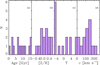 |
Fig. 5. Distribution of ages (panel a), metallicities (panel b), morphological type (panel c), and velocity dispersion (panel d) for the stellar component in the sample of galaxies. |
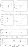 |
Fig. 6. Upper panels: comparison between our measurements of Lick line-strength indices and those available in literature (Tables 3 and A.1–A.4). For uniformity we only show literature sources that include multiple galaxies from our sample. The plot intervals reflect the ranges of values from our measurements. Bottom panels: difference between our heliocentric velocities and velocity dispersion in the central region of the sample galaxies and those from literature as a function of the literature values. The average difference of 39 measurements after removing three outliers is consistent with zero (−7 ± 29 km s−1). |
6. Summary
In this paper we present new high-quality UV–VIS–NIR spectroscopy of a set of well-studied galaxies spanning a large range of ages, metallicities, and mass, and ranging from ellipticals to spirals (Fig. 5). This satisfies our aim which is to create an atlas of spectra for a variety of galaxies to be used as a template to investigate their spectral properties homogeneously from the optical to the NIR.
Our X-shooter data set of combined optical–NIR range sampling the same spatial region of the galaxies minimize any systematic. The combination of wide spectral coverage and high S/N in our data is unique and unprecedented.
Such a dataset of spectra will be crucial to addressing important questions of the modern investigation concerning galaxy formation and evolution. Some relevant topics among others are the study of the slope of the IMF, the role of the AGB stars in tracing young stellar populations, the galaxy continuum, and the absorption features in the IR as complementary tools. These spectra will also be extremely useful as templates for stellar population modeling.
We also discussed a number of tests for the data quality validation to confirm the goodness and consistency of our galaxy spectra. As a consistency check, in Sect. 4, we compared the spectra of our galaxies with flux-calibrated spectra from the literature, finding a good match between them. For two galaxies of our sample, NGC 584 and NGC 3379, we estimated the quality of our data-processing in recovering the continuum shape of the spectra. To perform this step we compared synthetic magnitudes derived from our spectra with observed apparent magnitudes reported by Brown et al. (2014). The results indicate good agreement for both galaxies. The flat residuals obtained as results of the ratio of products generated from different observations of the same galaxy are a strong indication of a lack of systematic effects in our data.
We measured velocities and velocity dispersions in the central region of the sample galaxies and compared them with the literature, finding good consistency within the scattered literature values reported from several sources.
The classical Lick line-strength indices in the optical range of the X-shooter spectra were also measured and their values were compared with different values from several literature sources. Their values of Hβ, Mgb, and ⟨Fe⟩ agree within the uncertainties with the same indices measured in this work. The observed small offset in the Hβ is due to the different or missing emission Hβ correction in the literature data.
Further in-depth analyses of the UV and the NIR parts of the spectra will be presented in a forthcoming paper.
Acknowledgments
This paper made extensive use of the SIMBAD Database at CDS (Centre de Données astronomiques) Strasbourg, the NASA/IPAC Extragalactic Database (NED) which is operated by the Jet Propulsion Laboratory, CalTech, under contract with NASA, and of the VizieR catalog access tool, CDS, Strasbourg, France. PF acknowledges support from the Conseil Scientifique de l’Observatoire de Paris and the Programme National Cosmologie et Galaxies (PNCG). L.M., A.P., E.M.C. and E.D.B. acknowledge financial support from Padua University through grants DOR1699945/16, DOR1715817/17, DOR1885254/18, and BIRD164402/16.
References
- Bernardi, M., Alonso, M. V., da Costa, L. N., et al. 2002, AJ, 123, 2990 [NASA ADS] [CrossRef] [Google Scholar]
- Bessell, M. S. 1990, PASP, 102, 1181 [NASA ADS] [CrossRef] [Google Scholar]
- Bonnefoy, M., Chauvin, G., Lagrange, A.-M., et al. 2014, A&A, 562, A127 [NASA ADS] [CrossRef] [EDP Sciences] [Google Scholar]
- Bottema, R. 1989, A&A, 221, 236 [NASA ADS] [Google Scholar]
- Brown, M. J. I., Moustakas, J., Smith, J.-D. T., et al. 2014, ApJS, 212, 18 [Google Scholar]
- Buser, R., & Kurucz, R. L. 1992, A&A, 264, 557 [NASA ADS] [Google Scholar]
- Cappellari, M., & Emsellem, E. 2004, PASP, 116, 138 [NASA ADS] [CrossRef] [Google Scholar]
- Castelli, F., Gratton, R. G., & Kurucz, R. L. 1997, A&A, 318, 841 [NASA ADS] [Google Scholar]
- Cesetti, M., Ivanov, V. D., Morelli, L., et al. 2009, A&A, 497, 41 [NASA ADS] [CrossRef] [EDP Sciences] [Google Scholar]
- Chen, Y.-P., Trager, S. C., Peletier, R. F., et al. 2014, A&A, 565, A117 [NASA ADS] [CrossRef] [EDP Sciences] [Google Scholar]
- Coelho, P., Barbuy, B., Meléndez, J., Schiavon, R. P., & Castilho, B. V. 2005, A&A, 443, 735 [NASA ADS] [CrossRef] [EDP Sciences] [Google Scholar]
- Cohen, M., Wheaton, W. A., & Megeath, S. T. 2003, AJ, 126, 1090 [NASA ADS] [CrossRef] [Google Scholar]
- Colless, M., Dalton, G., Maddox, S., et al. 2001, MNRAS, 328, 1039 [NASA ADS] [CrossRef] [Google Scholar]
- Colless, M., Peterson, B. A., Jackson, C., et al. 2003, ArXiv e-prints [arXiv:astro-ph/0306581] [Google Scholar]
- Conroy, C., & van Dokkum, P. 2012, ApJ, 747, 69 [NASA ADS] [CrossRef] [Google Scholar]
- Cushing, M. C., Rayner, J. T., & Vacca, W. D. 2005, ApJ, 623, 1115 [NASA ADS] [CrossRef] [Google Scholar]
- Davies, R. L., Burstein, D., Dressler, A., et al. 1987, ApJS, 64, 581 [NASA ADS] [CrossRef] [Google Scholar]
- Davies, B., Kudritzki, R.-P., Plez, B., et al. 2013, ApJ, 767, 3 [NASA ADS] [CrossRef] [Google Scholar]
- Doyon, R., Joseph, R. D., & Wright, G. S. 1994a, ApJ, 421, 101 [NASA ADS] [CrossRef] [Google Scholar]
- Doyon, R., Wright, G. S., & Joseph, R. D. 1994b, ApJ, 421, 115 [NASA ADS] [CrossRef] [Google Scholar]
- Engelbracht, C. W., Rieke, M. J., Rieke, G. H., Kelly, D. M., & Achtermann, J. M. 1998, ApJ, 505, 639 [NASA ADS] [CrossRef] [Google Scholar]
- Faber, S. M., Friel, E. D., Burstein, D., & Gaskell, C. M. 1985, ApJS, 57, 711 [NASA ADS] [CrossRef] [Google Scholar]
- Faber, S. M., Wegner, G., Burstein, D., et al. 1989, ApJS, 69, 763 [NASA ADS] [CrossRef] [Google Scholar]
- Falco, E. E., Kurtz, M. J., Geller, M. J., et al. 1999, PASP, 111, 438 [NASA ADS] [CrossRef] [Google Scholar]
- Franx, M., Illingworth, G., & Heckman, T. 1989, ApJ, 344, 613 [NASA ADS] [CrossRef] [Google Scholar]
- Freudling, W., Romaniello, M., Bramich, D. M., et al. 2013, A&A, 559, A96 [NASA ADS] [CrossRef] [EDP Sciences] [Google Scholar]
- Fukugita, M., Ichikawa, T., Gunn, J. E., et al. 1996, AJ, 111, 1748 [NASA ADS] [CrossRef] [Google Scholar]
- Gavazzi, G., Zaccardo, A., Sanvito, G., Boselli, A., & Bonfanti, C. 2004, A&A, 417, 499 [NASA ADS] [CrossRef] [EDP Sciences] [Google Scholar]
- Gavazzi, G., Consolandi, G., Dotti, M., et al. 2013, A&A, 558, A68 [NASA ADS] [CrossRef] [EDP Sciences] [Google Scholar]
- Geballe, T. R., Kulkarni, S. R., Woodward, C. E., & Sloan, G. C. 1996, ApJ, 467, L101 [NASA ADS] [CrossRef] [Google Scholar]
- Goldoni, P., Royer, F., François, P., et al. 2006, Proc. SPIE, 6269, 62692K [CrossRef] [Google Scholar]
- Gonneau, A., Lançon, A., Trager, S. C., et al. 2016, A&A, 589, A36 [NASA ADS] [CrossRef] [EDP Sciences] [Google Scholar]
- Gorgas, J., Efstathiou, G., & Aragon Salamanca, A. 1990, MNRAS, 245, 217 [NASA ADS] [Google Scholar]
- Gorlova, N. I., Meyer, M. R., Rieke, G. H., & Liebert, J. 2003, ApJ, 593, 1074 [NASA ADS] [CrossRef] [Google Scholar]
- Guinouard, I., Horville, D., Puech, M., et al. 2006, Proc. SPIE, 6273, 62733R [CrossRef] [Google Scholar]
- Hanson, M. M., Howarth, I. D., & Conti, P. S. 1997, ApJ, 489, 698 [NASA ADS] [CrossRef] [Google Scholar]
- Hanson, M. M., Luhman, K. L., & Rieke, G. H. 2002, ApJS, 138, 35 [NASA ADS] [CrossRef] [Google Scholar]
- Ho, L. C. 2007, ApJ, 668, 94 [NASA ADS] [CrossRef] [Google Scholar]
- Ho, L. C., Filippenko, A. V., & Sargent, W. L. 1995, ApJS, 98, 477 [NASA ADS] [CrossRef] [Google Scholar]
- Ho, L. C., Greene, J. E., Filippenko, A. V., & Sargent, W. L. W. 2009, ApJS, 183, 1 [NASA ADS] [CrossRef] [Google Scholar]
- Huchra, J. P., Macri, L. M., Masters, K. L., et al. 2012, ApJS, 199, 26 [NASA ADS] [CrossRef] [Google Scholar]
- Hyvönen, T., Kotilainen, J. K., Reunanen, J., & Falomo, R. 2009, A&A, 499, 417 [NASA ADS] [CrossRef] [EDP Sciences] [Google Scholar]
- Imanishi, M., & Alonso-Herrero, A. 2004, ApJ, 614, 122 [NASA ADS] [CrossRef] [Google Scholar]
- Ivanov, V. D., Rieke, G. H., Groppi, C. E., et al. 2000, ApJ, 545, 190 [NASA ADS] [CrossRef] [Google Scholar]
- Ivanov, V. D., Rieke, M. J., Engelbracht, C. W., et al. 2004, ApJS, 151, 387 [NASA ADS] [CrossRef] [Google Scholar]
- Johnson, H. L., & Méndez, M. E. 1970, AJ, 75, 785 [NASA ADS] [CrossRef] [Google Scholar]
- Johansson, J., Thomas, D., & Maraston, C. 2010, MNRAS, 406, 165 [NASA ADS] [CrossRef] [Google Scholar]
- Jones, D. H., Read, M. A., Saunders, W., et al. 2009, MNRAS, 399, 683 [NASA ADS] [CrossRef] [Google Scholar]
- Joyce, R. R., Hinkle, K. H., Wallace, L., Dulick, M., & Lambert, D. L. 1998, AJ, 116, 2520 [NASA ADS] [CrossRef] [Google Scholar]
- Kelson, D. D. 2003, PASP, 115, 688 [NASA ADS] [CrossRef] [Google Scholar]
- Kennicutt, Jr., R. C. 1992, ApJS, 79, 255 [NASA ADS] [CrossRef] [Google Scholar]
- Kleinmann, S. G., & Hall, D. N. B. 1986, ApJS, 62, 501 [NASA ADS] [CrossRef] [Google Scholar]
- Kotilainen, J. K., Reunanen, J., Laine, S., & Ryder, S. D. 2001, A&A, 366, 439 [NASA ADS] [CrossRef] [EDP Sciences] [Google Scholar]
- Kotilainen, J. K., Hyvönen, T., Reunanen, J., & Ivanov, V. D. 2012, MNRAS, 425, 1057 [NASA ADS] [CrossRef] [Google Scholar]
- Lambert, D. L., Gustafsson, B., Eriksson, K., & Hinkle, K. H. 1986, ApJS, 62, 373 [NASA ADS] [CrossRef] [Google Scholar]
- Lançon, A., & Mouhcine, M. 2000, Massive Stellar Clusters, eds. A. Lançon, & C. M. Boily, ASP Conf. Ser., 211, 34 [Google Scholar]
- Lançon, A., & Wood, P. R. 2000, A&AS, 146, 217 [NASA ADS] [CrossRef] [EDP Sciences] [Google Scholar]
- Leitherer, C., Alloin, D., Alvensleben, U. F. V., et al. 1996, PASP, 108, 996 [NASA ADS] [CrossRef] [Google Scholar]
- Lejeune, T., Cuisinier, F., & Buser, R. 1997, A&AS, 125, 229 [NASA ADS] [CrossRef] [EDP Sciences] [Google Scholar]
- Lejeune, T., Cuisinier, F., & Buser, R. 1998, A&AS, 130, 65 [NASA ADS] [CrossRef] [EDP Sciences] [Google Scholar]
- Lyubenova, M., Kuntschner, H., Rejkuba, M., et al. 2010, A&A, 510, A19 [NASA ADS] [CrossRef] [EDP Sciences] [Google Scholar]
- Lyubenova, M., Kuntschner, H., Rejkuba, M., et al. 2012, A&A, 543, A75 [NASA ADS] [CrossRef] [EDP Sciences] [Google Scholar]
- Makarov, D., Prugniel, P., Terekhova, N., Courtois, H., & Vauglin, I. 2014, A&A, 570, A13 [CrossRef] [EDP Sciences] [Google Scholar]
- Maraston, C. 2005, MNRAS, 362, 799 [NASA ADS] [CrossRef] [Google Scholar]
- Maraston, C. 2011, Why Galaxies Care about AGB Stars II: Shining Examples and Common Inhabitants, eds. F. Kerschbaum, T. Lebzelter, & R. F. Wing, ASP Conf. Ser., 445, 391 [NASA ADS] [Google Scholar]
- Maraston, C., & Strömbäck, G. 2011, MNRAS, 418, 2785 [NASA ADS] [CrossRef] [Google Scholar]
- Maraston, C., Daddi, E., Renzini, A., et al. 2006, ApJ, 652, 85 [NASA ADS] [CrossRef] [Google Scholar]
- Mármol-Queraltó, E., Cardiel, N., Sánchez-Blázquez, P., et al. 2009, ApJ, 705, L199 [CrossRef] [Google Scholar]
- Mason, R. E., Rodríguez-Ardila, A., Martins, L., et al. 2015, ApJS, 217, 13 [NASA ADS] [CrossRef] [Google Scholar]
- McElroy, D. B. 1995, ApJS, 100, 105 [NASA ADS] [CrossRef] [Google Scholar]
- Mehlert, D., Thomas, D., Saglia, R. P., Bender, R., & Wegner, G. 2003, A&A, 407, 423 [NASA ADS] [CrossRef] [EDP Sciences] [Google Scholar]
- Melbourne, J., Williams, B. F., Dalcanton, J. J., et al. 2012, ApJ, 748, 47 [NASA ADS] [CrossRef] [Google Scholar]
- Meneses-Goytia, S., Peletier, R. F., Trager, S. C., et al. 2015a, A&A, 582, A96 [NASA ADS] [CrossRef] [EDP Sciences] [Google Scholar]
- Meneses-Goytia, S., Peletier, R. F., Trager, S. C., & Vazdekis, A. 2015b, A&A, 582, A97 [NASA ADS] [CrossRef] [EDP Sciences] [Google Scholar]
- Messineo, M., Davies, B., Ivanov, V. D., et al. 2009, ApJ, 697, 701 [NASA ADS] [CrossRef] [Google Scholar]
- Meyer, M. R., Edwards, S., Hinkle, K. H., & Strom, S. E. 1998, ApJ, 508, 397 [NASA ADS] [CrossRef] [Google Scholar]
- Morelli, L., Halliday, C., Corsini, E. M., et al. 2004, MNRAS, 354, 753 [NASA ADS] [CrossRef] [Google Scholar]
- Morelli, L., Pompei, E., Pizzella, A., et al. 2008, MNRAS, 389, 341 [NASA ADS] [CrossRef] [Google Scholar]
- Morelli, L., Pizzella, A., Corsini, E. M., et al. 2015, Astron. Nachr., 336, 208 [NASA ADS] [CrossRef] [Google Scholar]
- Morelli, L., Parmiggiani, M., Corsini, E. M., et al. 2016, MNRAS, 463, 4396 [NASA ADS] [CrossRef] [Google Scholar]
- Mould, J., Reynolds, T., Readhead, T., et al. 2012, ApJS, 203, 14 [NASA ADS] [CrossRef] [Google Scholar]
- Oppenheimer, B. R., Kulkarni, S. R., Matthews, K., & Nakajima, T. 1995, Science, 270, 1478 [NASA ADS] [CrossRef] [PubMed] [Google Scholar]
- Origlia, L., Moorwood, A. F. M., & Oliva, E. 1993, A&A, 280, 536 [NASA ADS] [Google Scholar]
- Ramirez, S. V., Depoy, D. L., Frogel, J. A., Sellgren, K., & Blum, R. D. 1997, AJ, 113, 1411 [NASA ADS] [CrossRef] [Google Scholar]
- Rayner, J. T., Cushing, M. C., & Vacca, W. D. 2009, ApJS, 185, 289 [NASA ADS] [CrossRef] [Google Scholar]
- Reunanen, J., Kotilainen, J. K., & Prieto, M. A. 2002, MNRAS, 331, 154 [NASA ADS] [CrossRef] [Google Scholar]
- Reunanen, J., Kotilainen, J. K., & Prieto, M. A. 2003, MNRAS, 343, 192 [NASA ADS] [CrossRef] [Google Scholar]
- Rieke, G. H., Lebofsky, M. J., Thompson, R. I., Low, F. J., & Tokunaga, A. T. 1980, ApJ, 238, 24 [NASA ADS] [CrossRef] [Google Scholar]
- Rieke, G. H., Lebofsky, M. J., & Walker, C. E. 1988, ApJ, 325, 679 [NASA ADS] [CrossRef] [Google Scholar]
- Riffel, R., Rodríguez-Ardila, A., & Pastoriza, M. G. 2006, A&A, 457, 61 [NASA ADS] [CrossRef] [EDP Sciences] [Google Scholar]
- Riffel, R., Bonatto, C., Cid Fernandes, R., Pastoriza, M. G., & Balbinot, E. 2011a, MNRAS, 411, 1897 [NASA ADS] [CrossRef] [Google Scholar]
- Riffel, R., Ruschel-Dutra, D., Pastoriza, M. G., et al. 2011b, MNRAS, 410, 2714 [NASA ADS] [CrossRef] [Google Scholar]
- Riffel, R., Mason, R. E., Martins, L. P., et al. 2015a, MNRAS, 450, 3069 [NASA ADS] [CrossRef] [Google Scholar]
- Riffel, R. A., Ho, L. C., Mason, R., et al. 2015b, MNRAS, 446, 2823 [NASA ADS] [CrossRef] [Google Scholar]
- Röck, B., Vazdekis, A., Peletier, R. F., Knapen, J. H., & Falcón-Barroso, J. 2015, MNRAS, 449, 2853 [NASA ADS] [CrossRef] [Google Scholar]
- Röck, B., Vazdekis, A., Ricciardelli, E., et al. 2016, A&A, 589, A73 [NASA ADS] [CrossRef] [EDP Sciences] [Google Scholar]
- Santos, J. F. C. J., Alloin, D., Bica, E., & Bonatto, C. 2002, in Extragalactic Star Clusters, eds. D. P. Geisler, E. K. Grebel, & D. Minniti, IAU Symp., 207, 1 [NASA ADS] [Google Scholar]
- Sarzi, M., Falcón-Barroso, J., Davies, R. L., et al. 2006, MNRAS, 366, 1151 [Google Scholar]
- Schechter, P. L. 1983, ApJS, 52, 425 [NASA ADS] [CrossRef] [Google Scholar]
- Sharples, R., Bender, R., Agudo Berbel, A., et al. 2013, The Messenger, 151, 21 [NASA ADS] [Google Scholar]
- Silva, D. R., Kuntschner, H., & Lyubenova, M. 2008, ApJ, 674, 194 [NASA ADS] [CrossRef] [Google Scholar]
- Skrutskie, M. F., Cutri, R. M., Stiening, R., et al. 2006, AJ, 131, 1163 [NASA ADS] [CrossRef] [Google Scholar]
- Smette, A., Sana, H., Noll, S., et al. 2015, A&A, 576, A77 [NASA ADS] [CrossRef] [EDP Sciences] [Google Scholar]
- Smith, R. J., Lucey, J. R., Hudson, M. J., Schlegel, D. J., & Davies, R. L. 2000, MNRAS, 313, 469 [NASA ADS] [CrossRef] [Google Scholar]
- Smith, R. J., Alton, P., Lucey, J. R., Conroy, C., & Carter, D. 2015, MNRAS, 454, L71 [NASA ADS] [CrossRef] [Google Scholar]
- Tamblyn, P., Rieke, G. H., Hanson, M. M., et al. 1996, ApJ, 456, 206 [NASA ADS] [CrossRef] [Google Scholar]
- Terlevich, R., Davies, R. L., Faber, S. M., & Burstein, D. 1981, MNRAS, 196, 381 [NASA ADS] [CrossRef] [Google Scholar]
- Terndrup, D. M., Frogel, J. A., & Whitford, A. E. 1991, ApJ, 378, 742 [NASA ADS] [CrossRef] [Google Scholar]
- Thomas, D., Maraston, C., & Bender, R. 2003, MNRAS, 339, 897 [NASA ADS] [CrossRef] [Google Scholar]
- Trager, S. C., Worthey, G., Faber, S. M., Burstein, D., & González, J. J. 1998, ApJS, 116, 1 [NASA ADS] [CrossRef] [MathSciNet] [Google Scholar]
- van Dokkum, P. G. 2001, PASP, 113, 1420 [NASA ADS] [CrossRef] [Google Scholar]
- Vanzi, L., & Rieke, G. H. 1997, ApJ, 479, 694 [NASA ADS] [CrossRef] [Google Scholar]
- Vanzi, L., Rieke, G. H., Martin, C. L., & Shields, J. C. 1996, ApJ, 466, 150 [NASA ADS] [CrossRef] [Google Scholar]
- Veilleux, S., Sanders, D. B., & Kim, D.-C. 1997a, ApJ, 484, 92 [NASA ADS] [CrossRef] [Google Scholar]
- Veilleux, S., Goodrich, R. W., & Hill, G. J. 1997b, ApJ, 477, 631 [NASA ADS] [CrossRef] [Google Scholar]
- Veilleux, S., Sanders, D. B., & Kim, D.-C. 1999, ApJ, 522, 139 [NASA ADS] [CrossRef] [Google Scholar]
- Vernet, J., Dekker, H., D’Odorico, S., et al. 2011, A&A, 536, A105 [NASA ADS] [CrossRef] [EDP Sciences] [Google Scholar]
- Villaume, A., Conroy, C., & Johnson, B. D. 2015, ApJ, 806, 82 [NASA ADS] [CrossRef] [Google Scholar]
- Wallace, L., & Hinkle, K. 1997, ApJS, 111, 445 [NASA ADS] [CrossRef] [Google Scholar]
- Wallace, L., & Hinkle, K. 2002, AJ, 124, 3393 [NASA ADS] [CrossRef] [Google Scholar]
- Wallace, L., Meyer, M. R., Hinkle, K., & Edwards, S. 2000, ApJ, 535, 325 [NASA ADS] [CrossRef] [MathSciNet] [Google Scholar]
- Wegner, G., Colless, M., Saglia, R. P., et al. 1999, MNRAS, 305, 259 [NASA ADS] [CrossRef] [Google Scholar]
- Wegner, G., Bernardi, M., Willmer, C. N. A., et al. 2003, AJ, 126, 2268 [NASA ADS] [CrossRef] [Google Scholar]
- Worthey, G. 1994, ApJS, 95, 107 [NASA ADS] [CrossRef] [Google Scholar]
- Worthey, G., Faber, S. M., & Gonzalez, J. J. 1992, ApJ, 398, 69 [NASA ADS] [CrossRef] [Google Scholar]
- Worthey, G., Faber, S. M., Gonzalez, J. J., & Burstein, D. 1994, ApJS, 94, 687 [NASA ADS] [CrossRef] [Google Scholar]
- York, D. G., Adelman, J., Anderson, Jr., J. E., et al. 2000, AJ, 120, 1579 [CrossRef] [Google Scholar]
- Zamora, O., García-Hernández, D. A., Allende Prieto, C., et al. 2015, AJ, 149, 181 [NASA ADS] [CrossRef] [Google Scholar]
- Zibetti, S., Gallazzi, A., Charlot, S., Pierini, D., & Pasquali, A. 2013, MNRAS, 428, 1479 [NASA ADS] [CrossRef] [Google Scholar]
Appendix A: Literature data for the sample galaxies
Previous measurements of the heliocentric velocities VH for the sample galaxies.
Previous measurements of the velocity dispersions σV for the sample galaxies.
Previous measurements of the Hβ and Mg2 line-strength indices for the sample galaxies.
Previous measurements of the spectral indices Mgb, Mg , Fe5270 and Fe5335 for sample galaxies.
List of the available spectra of the sample galaxies.
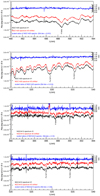 |
Fig. A.1. Comparison of selected regions of the spectra from two observations of NGC 1425 (top two panels) and NGC 4415 (bottom two panels). |
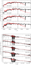 |
Fig. A.2. Further comparison of our spectra (black) with literature (red) spectra from Jones et al. (2009) for some of the galaxies in common between both samples (top panel) and from Cesetti et al. (2009) for our bonafide ellipticals and their average spectrum of ellipticals. The literature spectra were always scaled to match the median flux level of our spectra. |
Appendix B: Spectra of the sample galaxies
Appendix C: Apparent central colors of the sample galaxies
Apparent colors for the central 1.3″ × 4″ apertures of the galaxies in our sample, derived from the X-shooter spectra, in the following photometric systems: UBVRI Bessel (Bessell 1990), JHKs 2MASS (Skrutskie et al. 2006), ugriz SDSS (Bessell 1990) and again JHKs 2MASS (Skrutskie et al. 2006), but converted to AB magnitudes.
All Tables
Central values of the velocity, dispersion, line-strength indices, age, and metallicity of the sample galaxies measured within an aperture of radius 0.3 re.
Previous measurements of the heliocentric velocities VH for the sample galaxies.
Previous measurements of the Hβ and Mg2 line-strength indices for the sample galaxies.
Previous measurements of the spectral indices Mgb, Mg, Fe5270 and Fe5335 for sample galaxies.
Apparent colors for the central 1.3″ × 4″ apertures of the galaxies in our sample, derived from the X-shooter spectra, in the following photometric systems: UBVRI Bessel (Bessell 1990), JHKs 2MASS (Skrutskie et al. 2006), ugriz SDSS (Bessell 1990) and again JHKs 2MASS (Skrutskie et al. 2006), but converted to AB magnitudes.
All Figures
|
Fig. 1. Spectra of the sample galaxies in different wavelength ranges. Each spectrum is normalized to unity, shifted for displaying purposes, and labeled with the NGC number of the galaxy. The spectra at the top of each panel are the average of the sample spectra (see Sect. 3). |
| In the text | |
|
Fig. 2. Comparison between our optical spectra (black lines) with literature spectra (red lines) scaled to match the flux level of ours. Top panels: spectra of NGC 3379 from different sources as given in the labels. Bottom panels: spectra of the four galaxies in common with Ho et al. (1995). Their spectra consist of two portions, which we separately scaled to match our spectrum. |
| In the text | |
|
Fig. 3. Comparison between the synthetic apparent magnitudes derived from our spectra and observed apparent magnitudes reported by Brown et al. (2014) for NGC 584 (open circles) and NGC 3379 (solid dots). |
| In the text | |
|
Fig. 4. A comparison of synthetic broad band colors generated from our spectra and apparent colors form the literature, listed in Table C.1. |
| In the text | |
|
Fig. 5. Distribution of ages (panel a), metallicities (panel b), morphological type (panel c), and velocity dispersion (panel d) for the stellar component in the sample of galaxies. |
| In the text | |
|
Fig. 6. Upper panels: comparison between our measurements of Lick line-strength indices and those available in literature (Tables 3 and A.1–A.4). For uniformity we only show literature sources that include multiple galaxies from our sample. The plot intervals reflect the ranges of values from our measurements. Bottom panels: difference between our heliocentric velocities and velocity dispersion in the central region of the sample galaxies and those from literature as a function of the literature values. The average difference of 39 measurements after removing three outliers is consistent with zero (−7 ± 29 km s−1). |
| In the text | |
|
Fig. A.1. Comparison of selected regions of the spectra from two observations of NGC 1425 (top two panels) and NGC 4415 (bottom two panels). |
| In the text | |
|
Fig. A.2. Further comparison of our spectra (black) with literature (red) spectra from Jones et al. (2009) for some of the galaxies in common between both samples (top panel) and from Cesetti et al. (2009) for our bonafide ellipticals and their average spectrum of ellipticals. The literature spectra were always scaled to match the median flux level of our spectra. |
| In the text | |
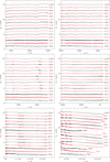 |
Fig. B.1. As in Fig. 1, but for the remaining spectra of our sample galaxies. |
| In the text | |
Current usage metrics show cumulative count of Article Views (full-text article views including HTML views, PDF and ePub downloads, according to the available data) and Abstracts Views on Vision4Press platform.
Data correspond to usage on the plateform after 2015. The current usage metrics is available 48-96 hours after online publication and is updated daily on week days.
Initial download of the metrics may take a while.