| Issue |
A&A
Volume 621, January 2019
|
|
|---|---|---|
| Article Number | A134 | |
| Number of page(s) | 7 | |
| Section | Stellar structure and evolution | |
| DOI | https://doi.org/10.1051/0004-6361/201833786 | |
| Published online | 21 January 2019 | |
Study of the X-ray pulsar IGR J19294+1816 with NuSTAR: Detection of cyclotron line and transition to accretion from the cold disk
1
Department of Physics and Astronomy, University of Turku, 20014 Turku, Finland
e-mail: This email address is being protected from spambots. You need JavaScript enabled to view it.
2
Space Research Institute of the Russian Academy of Sciences, Profsoyuznaya Str. 84/32, 117997 Moscow, Russia
3
Institut für Astronomie und Astrophysik, Universität Tübingen, Sand 1, 72076 Tübingen, Germany
4
Leiden Observatory, Leiden University, 2300 RA Leiden, The Netherlands
5
Pulkovo Observatory of the Russian Academy of Sciences, 196140 Saint Petersburg, Russia
Received:
6
July
2018
Accepted:
19
November
2018
Abstract
In the work we present the results of two deep broadband observations of the poorly studied X-ray pulsar IGR J19294+1816 obtained with the NuSTAR observatory. The source was observed during Type I outburst and in the quiescent state. In the bright state a cyclotron absorption line in the energy spectrum was discovered at Ecyc = 42.8 ± 0.7 keV. Spectral and timing analysis prove the ongoing accretion also during the quiescent state of the source. Based on the long-term flux evolution, particularly on the transition of the source to the bright quiescent state with luminosity around 1035 erg s−1, we conclude that IGR J19294+1816 switched to the accretion from the “cold” accretion disk between Type I outbursts. We also report the updated orbital period of the system.
Key words: accretion / accretion disks / magnetic fields / stars: individual: IGR J19294+1816 / X-rays: binaries
© ESO 2019
1. Introduction
Timing and spectral properties of radiation generated by accreting objects carry information about physical and geometrical properties of the systems. In the case of the highly magnetized neutron stars known as X-ray pulsars (XRPs) detailed analysis of the emission in different luminosity states allows us to investigate physical processes both very close to the neutron star (NS) and at the boundary between accretion disk and the magnetosphere. Moreover, observational appearance of these physical processes may drastically depend on the properties of the particular XRP (such as pulse period and magnetic field strength), reflecting different regimes of matter interaction with magnetic field and radiation.
Accurate knowledge of the magnetic field strength is crucial for application of physical models describing such interaction. Here we have used high-quality NuSTAR data in order to accurately measure the magnetic field of the poorly studied transient XRP IGR J19294+1816. This information is further used to fill the gap in our knowledge of how pulsars with intermediate spin periods interact with the accretion disk. In particular, we aim to verify our earlier prediction that there is a critical spin period (around 10 s for standard magnetic field strength) dividing all XRPs into two families: (i) short-spin pulsars able to switch to the “propeller” regime at the final stages of their outbursts, and (ii) long-spin ones continuing to accrete stably from the “cold” accretion disk (Tsygankov et al. 2017a). IGR J19294+1816 with ∼12.4 s spin period (Rodriguez et al. 2009; Strohmayer et al. 2009) is an excellent candidate to fill the gap between these two families of XRPs.
IGR J19294+1816 was discovered by the INTEGRAL observatory on 2009 March 27 (Turler et al. 2009). Analysis of the archival Swift/XRT data of this region revealed relatively bright source showing evidence of pulsations at ∼12.4 s (Rodriguez et al. 2009). The pulsar nature of the source was confirmed later by Strohmayer et al. (2009). Long-term flux variability with period of about 117.2 d was discovered by the Swift/BAT monitor and was associated with orbital modulation (Corbet & Krimm 2009). Based on the transient behavior of IGR J19294+1816 and its position on the Corbet diagram an assumption about a Be/XRP nature of the source was made. The NIR spectroscopy presented by Rodes-Roca et al. (2018) directly confirmed this hypothesis, resulting in the identification of the optical companion in the system with a B1Ve star located at the far edge of the Perseus arm at a distance of d = 11 ± 1 kpc.
The relative faintness of IGR J19294+1816 did not allow to make any conclusions regarding the physical properties of the NS in the system up to date. Only tentative detection of the cyclotron absorption line at ∼35.5 keV was reported based on the deviation of the source spectrum from a power law at higher energies using the RXTE data (Roy et al. 2017). In this work we have used long-term Swift/XRT monitoring observations to characterize accretion regimes in the system as well as two dedicated deep NuSTAR observations to describe properties of the NS in the hard X-ray range for the first time.
2. Data analysis
This work is based on the data from the XRT telescope (Burrows et al. 2005) onboard the Neil Gehrels Swift Observatory (Gehrels et al. 2004) obtained during monitoring programs performed during and after the Type I outbursts in 2010 and 2017–2018, as well as two NuSTAR (Harrison et al. 2013) observations, the first of which was nearly simultaneous with that of Swift/XRT in March 2018.
2.1. Swift/XRT data
High sensitivity and flexibility of the Swift/XRT telescope allow us to carry out long-term monitoring programs probing source flux evolution in a very broad range. Particularly, it permitted us to investigate the transition of IGR J19294+1816 from the outburst to the quiescent state. Because of the low count rates all XRT observations were performed in the photon counting (PC) mode and automatically reduced using the online tools (Evans et al. 2009) provided by the UK Swift Science Data Centre1.
The data sample consists of observations performed after Type I outbursts occurred in the end of 2010 and 2017. The corresponding light curves are shown in the top panel of Fig. 1. Luminosity was calculated from the bolometric (see below) and absorption corrected flux determined based on the results of spectral fitting in XSPEC package assuming absorbed power law model and distance to the source d = 11 kpc (Rodes-Roca et al. 2018). Taking into account low count statistics we binned the spectra in the 0.5–10 keV range to have at least one count per energy bin and fitted them using W-statistic (Wachter et al. 1979)2.
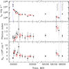 |
Fig. 1. Top panel: bolometrically corrected light curve of IGR J19294+1816 obtained with the Swift/XRT telescope in 2010 (left side) and 2017–2018 (right side) assuming distance to the source 11 kpc. Blue dotted lines show moments of periastron passages (see Sect. 3.4). Middle and bottom panels: corresponding evolution of the power law photon index and absorption value assuming an absorbed power law model. Black points correspond to individual XRT observations, whereas red open circles represent parameters obtained from the averaging of a few nearby observations with low count statistics. Vertical dash-dotted lines show moments of the NuSTAR observations. |
In order to convert the observed 0.5–10 keV flux into the total X-ray luminosity and, correspondingly, mass accretion rate, we estimated the bolometric correction factors using two broadband NuSTAR observations performed in the quiescent and outburst states. Flux ratio between these two states was more than 50. As discussed below (see Sect. 3.2, the broadband spectrum of the source depends slightly on its intensity, that is reflected in the flux-dependent bolometric correction factors. Particularly, in the quiescent state with the unabsorbed 0.5–10 keV flux around F0.5−10 keV ∼ 4 × 10⁻¹² erg s−1 cm−2 the bolometric correction (defined as the ratio of fluxes in the 0.5–100 to 0.5–10 keV ranges) was Kbol ∼ 1.8, whereas during the second observation (F0.5−10 keV ∼ 1.1 × 10⁻¹⁰ erg s−1 cm−2) it increased up to ∼2.5. Assuming a linear dependence of the bolometric correction on the logarithm of flux in the 0.5–10 keV band a simple equation can be obtained for Kbol = 7.5 + 0.5 log(F0.5−10 keV). In the following analysis we applied this correction to all XRT observations and refer to the bolometrically corrected fluxes and luminosities, unless stated otherwise.
2.2. NuSTAR data
The NuSTAR instruments include two co-aligned identical X-ray telescope systems allowing to focus X-ray photons in a wide energy range from 3 to 79 keV (Harrison et al. 2013). Thanks to the unprecedented sensitivity in hard X-rays, NuSTAR is ideally suited for the broadband spectroscopy of different types of objects, including XRPs, and searching for the cyclotron lines in their spectra.
The X-ray pulsar IGR J19294+1816 has been observed with NuSTAR twice in March 2018 (see Table 1). First observation (ObsID 90401306002) was performed on March 3, in the very end of the orbital cycle when the source was in the lowest state ever observed. Second observation (ObsID 90401306004) occurred two weeks later, on March 16, when the source entered another regular Type I outburst. In this state IGR J19294+1816 was about 50 times brighter than the first observation.
NuSTAR observations of IGR J19294+1816.
The raw observational data were processed following the standard data reduction procedures described in NuSTAR user guide and the standard NuSTAR Data Analysis Software (NUSTARDAS) v1.6.0 provided under HEASOFT V6.24 with the CALDB version 20180419.
The source spectra were extracted from the source-centered circular region with radius of 47″ using the NUPRODUCTS routine. The extraction radius was chosen to optimize the signal to noise ratio above 30 keV. The background was extracted from a source-free circular region with radius of 165″ in the corner of the field of view.
3. Results
The bolometrically and absorption corrected lightcurve of IGR J19294+1816 obtained with the Swift/XRT telescope during the monitoring programs in 2010 and 2017–2018 is shown on the top panel of Fig. 1. The overall behavior of the source can be divided into two main states: (i) quiescent state with luminosity around 1035 erg s−1, and (ii) outbursts associated with the periastron passage (Type I outbursts) with peak luminosity reaching ∼1037 erg s−1. Middle and bottom panels of the figure show the corresponding evolution of the photon index and absorption value measured in the 0.5–10 keV energy band assuming absorbed power law model (PHABS × POW in XSPEC). As can be seen, this simple spectral model fits the data in XRT range at all observed flux levels. Although some spectral variability is observed, the transition to the thermal spectrum, expected in the case of cooling NS surface (see e.g., Wijnands & Degenaar 2016), is never observed in IGR J19294+1816, strongly indicating the continuation of accretion in the quiescent state.
Similar behavior with transition of the source to the stable accretion between Type I outbursts has recently been discovered in another Be/XRP GRO J1008–57 and interpreted as accretion from the cold disk (Tsygankov et al. 2017a). To study this process in more details deep broadband observations were requested in these two states of IGR J19294+1816. Despite an only 13-day gap between observations NuSTAR found the source in completely different states with luminosities LX = 6.7 × 1034 erg s−1 (ObsID 90401306002; low state) and LX = 3.4 × 1036 erg s−1 (ObsID 90401306004; high state). The light curves of the source obtained from the NuSTAR data in full energy range do not reveal any strong variability. The source flux remains stable within a factor of around two in both observations.
3.1. Pulse profile and pulsed fraction
No binary orbital parameters except orbital period are known for IGR J19294+1816. Therefore pulsations were searched in the light curves with only barycentric correction applied and resulting periods might be biased due to orbital motion of the source. Pulsations were detected with high significance in both states. The obtained count statistics of NuSTAR data allowed us to reconstruct pulse profiles in several energy bands from 3 to 50 keV for each observation using spin periods P1 = 12.4832(2) s and P2 = 12.4781(1) s for the low and high states, respectively (see Fig. 2). Uncertainties for the pulse periods were determined from large number of simulated light curves following procedures described in Boldin et al. (2013).
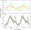 |
Fig. 2. Pulse profiles of IGR J19294+1816 obtained with NuSTAR in different energy bands during low (panel a) and high (panel b) states. Different colors correspond to different energy bands: 3–10 keV (red), 10–18 keV (yellow), 18–27 keV (green), 27–37 keV (blue), 37–50 keV (black). |
The shape of the pulse profile is very similar in different states. At the same time it demonstrates a clear dependence on energy. Below ∼10 keV the profile has broad single peak. With the increase of energy the profile structure becomes more complicated. Specifically, it becomes double-peaked with peaks separated by 0.5 in pulsar phase.
The pulsed fraction3 as a function of energy is shown in Fig. 3. For both states the increase of the pulsed fraction toward higher energies is observed, that is typical behavior for the majority of XRPs (Lutovinov & Tsygankov 2009). We note that during the low state the pulsed fraction was significantly lower. Similar drop of the pulsed fraction in the low state was found in GRO J1008–57 reinforcing the similarity between these two sources.
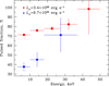 |
Fig. 3. Dependence of the pulsed fraction of IGR J19294+1816 on energy as seen by NuSTAR in the low (blue squares) and the high (red circles) states. |
3.2. Phase averaged spectral analysis
Discovery of the cyclotron resonance scattering feature at ∼36 keV in the spectrum of the source has been claimed by Roy et al. (2017) based on the observed deviation of the RXTE/PCA continuum from a power law above ∼30 keV. The choice of the continuum model by the authors appears, however, to be extremely odd, because X-ray spectra of all known XRPs exhibit a cutoff above ∼15−20 keV (see e.g., Nagase 1989; Filippova et al. 2005). The cutoff is actually expected for a spectrum produced through comptonization in hot emission region (e.g., Sunyaev & Titarchuk 1980; Meszaros & Nagel 1985). It is extremely likely, therefore, that the cyclotron line included in the model in practice simply mimicked the cutoff, and thus is not real.
To verify this possibility, we re-analyzed the RXTE observation 95438-01-01-00 (MJD 55499.46) where the line appeared to be most significant. Indeed, we found that the broadband RXTE/PCA continuum is perfectly well described with an absorbed cut-off power law model with no additional features required by the fit. Alternatively, it can be described with one of the comptonization models such as COMPTT or NTHCOMP with χ2/d.o.f. ∼ 0.8 (in all cases the fluorescence iron line was also included in the fit with the energy fixed at 6.4 keV and width at 0.1 keV). On the other hand, we verified that it is indeed possible to model the spectrum with a combination of a power law and CYCLABS model, however, not only the fit quality is considerably worse in this case but also the line itself gets unreasonably deep. We conclude, therefore, that the claim of the cyclotron line discovery by Roy et al. (2017) is unsupported by the data used by the authors, which has insufficient statistics.
On the other hand, NuSTAR data provide much better statistics and allow us to conduct a much more sensitive search for the possible cyclotron lines in the source spectrum. Similarly to RXTE, NuSTAR broadband spectrum can be well described with several continuum models. However, residuals around ∼40 keV in absorption are immediately apparent in phase-averaged spectrum from observation 90401306004 (i.e., when the source was in bright state) irrespective on the continuum model used. The fit can be greatly improved by inclusion of a Gaussian absorption line in the model. The width of the line depends slightly on the continuum model, but the feature is always significantly detected at the same energy. For the NTHCOMP continuum model, an absorption line with energy 42.9(1) keV, width of 6.9(5) keV and optical depth at line center of τ = 1.3(2) improves the fit from χ2/d.o.f. = 1132/720 to χ2/d.o.f. = 766/717, which corresponds to probability of chance improvement of ∼3 × 10−79 according to MLR test (Protassov et al. 2002).
The feature is, therefore, highly significant. This is also the case with other continuum models, so we conclude that while the report by Roy et al. (2017) is erroneous, the source does have indeed a cyclotron line at ∼43 keV, which implies magnetic field of ∼5 × 10¹² G assuming gravitational redshift z = 0.35 for the typical NS parameters. Usage of the CYCLABS model instead of GABS results in slightly lower cyclotron energy about 40 keV. Such discrepancy between these two models is associated with the definition of the latter model, and was found in other studies (e.g., Tsygankov et al. 2012; Mushtukov et al. 2015). There is also some evidence for the harmonic at double energy in the residuals (see Fig. 4), although its significance is low with a false alarm probability of ∼2% (assuming the energy and width of the fundamental fixed to be double that of the fundamental, and even lower otherwise).
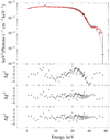 |
Fig. 4. Spectrum of IGR J19294+1816 obtained with the NuSTAR telescopes during the high state. The data from the two NuSTAR units are added together for plotting (but not for actual fit). The best-fitting residuals for models (top to bottom) without inclusion of the absorption feature, with fundamental only (at ∼42.8 keV; shown with the solid line in the top panel), and including the first harmonics (at ∼85 keV, dotted line in the top panel) are also shown. |
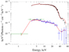 |
Fig. 5. Spectral energy distribution of IGR J19294+1816 obtained with the Swift/XRT and NuSTAR telescopes during the high (black dots) and low (blue and green dots) intensity states. The data from the two NuSTAR units are added together for plotting (but not for actual fit). Solid lines represent best-fit models for each observation including fundamental line only (see text). |
The counting statistics in the second observation, unfortunately, do not allow us to confidently detect the line, nor to constrain its parameters. Constraining the luminosity-related changes of the cyclotron line energy is, however, extremely interesting given the results reported previously for other sources (Tsygankov et al. 2006; Staubert et al. 2007; Klochkov et al. 2012). We thus attempted to estimate the line energy in the low state by formally including it in the fit, and modeling the high and low-state spectra simultaneously with the absorption column and cyclotron line width and depth linked between both observations (to reduce the number of free parameters). The fit results are presented in Table 2. We find the line energy to be consistent between the observations, although uncertainties for the low-state observation are, unfortunately, rather large. It is important to emphasize that the low counting statistics precludes significant detection of the line if only the second observation is considered. A deeper observation in quiescence would thus be required to firmly detect the line and to constrain its parameters.
Best-fit parameters for a PHABS*NTHCOMP model obtained for both observations.
3.3. Phase resolved spectral analysis
To investigate possible pulse phase dependence of spectral parameters in IGR J19294+1816 we performed phase resolved spectral analysis in the bright state (NuSTAR ObsID 90401306004). Phase bins for individual spectra were chosen based on the hardness ratio over the pulse. As can be seen from the two top panels in Fig. 6, there are four phase bins with significantly different values of hardness ratio, that can be a hint for significantly different spectral properties.
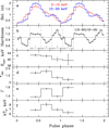 |
Fig. 6. Results of phase resolved spectroscopy of IGR J19294+1816 obtained with the NuSTAR telescope in the high intensity state. |
The obtained four spectra were fitted with the same model as in the case of phase averaged spectrum, that is, PHABS*(GAU+NTHCOMP*GABS) in XSPEC. Absorption parameter NH was free to vary and we did not find any evolution of its value over the pulse period. Because of low count statistics at high energies we froze the cyclotron line width at 6.8 keV determined from phase-averaged spectrum (see Table 2). Variability of the cyclotron line energy and optical depth is shown in Figs. 6c,d. The position of the cyclotron line does not exhibit strong dependence on the pulse phase, whereas depth of the line appears to vary significantly. In particular, the line is deepest at phases around 0.5–0.7 and is consistent with zero around phase 0.2. Parameters of the continuum (both Γ and kTe were free to vary) are significantly different at different phases, which is in line with observed hardness variations (see Figs. 6e,f). For the illustrative purposes we show all four spectra on one plot (see Fig. 7).
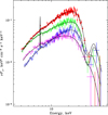 |
Fig. 7. Spectra of IGR J19294+1816 obtained in four pulse phases shown in Fig. 6. Phase bins 1, 2, 3, and 4 correspond to red, green, blue and black points, respectively. |
3.4. Orbital period
Orbital period of the source has been estimated by Corbet & Krimm (2009) at around 117 d based on the variability of Swift/BAT light curve. A lot of new data has been accumulated since 2009, which we exploited to refine the orbital period value. In particular, given the low duration and symmetric profile of the outbursts, we determined the time corresponding to the peak of each outburst in the light curve by fitting a Gaussian in the light curve (for orbital cycles exhibiting any excess around the peak). These times were then used to determine the orbital period using the phase connection technique as presented in Fig. 8. The orbital period was found to be 116.93(5) d, with the outburst peak epoch of MJD 53510.9(5), which is in line with earlier estimates (Corbet & Krimm 2009; Bozzo et al. 2011).
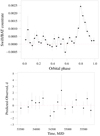 |
Fig. 8. Top panel: folded light curve of the source as observed by Swift/BAT. The zero phase here is arbitrary to make the peak clearly visible. Bottom panel: residuals to the linear fit of the outburst peak times determined as described in the text. |
4. Discussion
One of the main goals for our observational campaign of IGR J19294+1816 was to investigate the source behavior during its transition from the state of intensive accretion during Type I outbursts to the quiescent state between them. Particularly, transition to the propeller regime, when accretion is prohibited by the centrifugal barrier of the rotating NS magnetosphere, could be expected in the case of relatively strong magnetic field (Illarionov & Sunyaev 1975).
Observational appearance of transition to the propeller regime in classical XRP is very clear and is expressed in a sharp drop of the source luminosity by approximately two orders of magnitude, depending on the NS magnetic field (Stella et al. 1986; Tsygankov et al. 2016a,b; Lutovinov et al. 2017). A substantial softening of the energy spectrum is also expected from accretion dominated power law to the NS cooling generated blackbody (Tsygankov et al. 2016a). The threshold luminosity for the onset of the propeller regime is determined by the equality of the co-rotation and magnetospheric radii (see e.g., Campana et al. 2002)
 (1)
(1)
where P is pulsar’s rotational period in seconds, B12 is NS magnetic field strength in units of 1012 G, R6 is NS radius in units of 106 cm and M1.4 is the NS mass in units of 1.4 M⊙. The factor k relates the magnetospheric radius in the case of disk accretion to the classical Alfvén radius (Rm = kRA) and is usually assumed to be k = 0.5, which appears justified both from theoretical and observational points of view (see e.g., Ghosh & Lamb 1979; Doroshenko et al. 2014; Campana et al. 2018).
However, recently it was shown that propeller effect can be observed only in XRPs possessing relatively short spin period and/or strong magnetic field. In the opposite case the cooling front, caused by thermal-viscous instability (see review by Lasota 2001), is able to reach inner radius of the accretion disk resulting in the NS transition to the stable accretion from the cold (low-ionization) disk before centrifugal barrier is able to fully cease accretion (Tsygankov et al. 2017a). First example of such a behavior was recently discovered in the Be/XRP GRO J1008–57, whose spin period is ∼94 s.
Luminosity corresponding to the transition of the whole accretion disk to the cold state is determined by the inner radius of the disk and, therefore, by the strength of the NS magnetic field
 (2)
(2)
Below this level, the temperature in the accretion disk is lower than 6500 K at R > Rm (Tsygankov et al. 2017a).
As clearly seen from Eqs. (1) to (2) the behavior of the pulsar at low mass accretion rates is determined by the spin period of the NS and its magnetic field. Thanks to the robust determination of the NS magnetic field strength from the position of the cyclotron line we are able to apply physical models of the accretion disk interaction with magnetosphere in IGR J19294+1816. Substituting P = 12.4 s and B12 = 5 to Eqs. (1) and (2) one can get Lprop = 2.5 × 1035 erg s−1 and Lcold = 0.1 × 1035 erg s−1 for this source. We see that Lprop > Lcold, which means that the source is expected to switch to the propeller regime before the cooling wave will reach inner radius of the accretion disk causing transition to the stable accretion.
However, the observed long-term light curve of the source, shown in Fig. 1, clearly demonstrates the transition of the pulsar into stable state with luminosity around 2 × 1035 erg s−1 that is much higher than expected from quiescent NS in XRPs emitting its thermal energy (see e.g., Tsygankov et al. 2017b). This is clear indication that IGR J19294+1816 was able to switch to the accretion from the cold disk before the centrifugal barrier stopped the accretion.
The cold disk accretion scenario is also supported by the spectral and timing analysis. First of all, a hard power-law-like spectral shape strongly supports continuation of the accretion process. Just insignificant increase of the photon index in the low state is observed (see middle panel of Fig. 1). Also the pulsed fraction drops significantly in this state, possibly pointing to the increased emitting area. We note that both features of accretion from the cold disk mentioned were observed in GRO J1008–57 (Tsygankov et al. 2017a).
The solution of this discrepancy between an expected and actual behavior of the source can be in the proximity of IGR J19294+1816 parameters to the border between pulsars expected to transit to the propeller regime and ones able to accrete from the cold disk (see Fig. 3 from Tsygankov et al. 2017a). Therefore, substantial simplifications contained in Eqs. (1) and (2) may become important for such sources. Some of the caveats have already been discussed in Tsygankov et al. (2017a), others include neglection of the accretion torque and convection, which might affect inner disk temperature, and thus transitional luminosity. Detailed discussion of these factors is out of scope of this paper and will be published elsewhere.
Not only are Eqs. (1) and (2) very approximate, but also the effective magnetosphere radius and thus value of k are rather uncertain (see e.g., D’Aì et al. 2015; Chashkina et al. 2017; Filippova et al. 2017; Bozzo et al. 2018). Finally, transitional luminosity level also depends on the assumed distance, which is also poorly known in most cases. It is essential, therefore, to increase the sample of objects with intermediate spin periods observed in quiescence, preferably including monitoring the transition.
5. Conclusion
In the work we present the results of the long-term observational campaign of poorly studied XRP IGR J19294+1816 performed with the Swift/XRT telescope as well as two deep broadband observations obtained with the NuSTAR observatory. It is shown that between bright regular Type I outbursts with peak luminosity around 1037 erg s−1 the source resides in a stable state with luminosity around 1035 erg s−1. Spectral and timing properties of IGR J19294+1816 point to the ongoing accretion in this low state, which we interpreted as accretion from the cold (low-ionization) accretion disk (Tsygankov et al. 2017a). In the bright state a cyclotron absorption line in the energy spectrum was discovered at Ecyc = 42.8 ± 0.7 keV allowing us to estimate the NS magnetic field strength to around 5 × 10¹² G. We were also able to substantially refine the orbital period of the system based on the long-term Swift/BAT light curve of the source.
See XSPEC manual; https://heasarc.gsfc.nasa.gov/xanadu/ xspec/manual/XSappendixStatistics.html
PF = (Fmax − Fmin)/(Fmax + Fmin), where Fmax and Fmin are maximum and minimum fluxes in the pulse profile, respectively.
Acknowledgments
This work was supported by the grant 14.W03.31.0021 of the Ministry of Science and Higher Education of the Russian Federation. This research was also supported by the Academy of Finland travel grants 309228 and 317552 (ST, JP) and by the Netherlands Organization for Scientific Research Veni Fellowship (AAM). This work made use of data supplied by the UK Swift Science Data Centre at the University of Leicester. We also express our thanks to the NuSTAR and Swift teams for prompt scheduling and executing our observations.
References
- Boldin, P. A., Tsygankov, S. S., & Lutovinov, A. A. 2013, Astron. Lett., 39, 375 [NASA ADS] [CrossRef] [Google Scholar]
- Bozzo, E., Ferrigno, C., Falanga, M., & Walter, R. 2011, A&A, 531, A65 [NASA ADS] [CrossRef] [EDP Sciences] [Google Scholar]
- Bozzo, E., Ascenzi, S., Ducci, L., et al. 2018, A&A, 617, A126 [NASA ADS] [EDP Sciences] [Google Scholar]
- Burrows, D. N., Hill, J. E., Nousek, J. A., et al. 2005, Space Sci. Rev, 120, 165 [Google Scholar]
- Campana, S., Stella, L., Israel, G. L., et al. 2002, ApJ, 580, 389 [NASA ADS] [CrossRef] [Google Scholar]
- Campana, S., Stella, L., Mereghetti, S., & de Martino, D. 2018, A&A, 610, A46 [NASA ADS] [CrossRef] [EDP Sciences] [Google Scholar]
- Chashkina, A., Abolmasov, P., & Poutanen, J. 2017, MNRAS, 470, 2799 [NASA ADS] [CrossRef] [Google Scholar]
- Corbet, R. H. D., & Krimm, H. A. 2009, ATel, 2008 [Google Scholar]
- D’Aì, A., Di Salvo, T., Iaria, R., et al. 2015, MNRAS, 449, 4288 [NASA ADS] [CrossRef] [Google Scholar]
- Doroshenko, V., Santangelo, A., Doroshenko, R., et al. 2014, A&A, 561, A96 [NASA ADS] [CrossRef] [EDP Sciences] [Google Scholar]
- Evans, P. A., Beardmore, A. P., Page, K. L., et al. 2009, MNRAS, 397, 1177 [NASA ADS] [CrossRef] [Google Scholar]
- Filippova, E. V., Mereminskiy, I. A., Lutovinov, A. A., Molkov, S. V., & Tsygankov, S. S. 2017, Astron. Lett., 43, 706 [NASA ADS] [Google Scholar]
- Filippova, E. V., Tsygankov, S. S., Lutovinov, A. A., & Sunyaev, R. A. 2005, Astron. Lett., 31, 729 [NASA ADS] [CrossRef] [Google Scholar]
- Gehrels, N., Chincarini, G., Giommi, P., et al. 2004, ApJ, 611, 1005 [NASA ADS] [CrossRef] [Google Scholar]
- Ghosh, P., & Lamb, F. K. 1979, ApJ, 232, 259 [NASA ADS] [CrossRef] [Google Scholar]
- Harrison, F. A., Craig, W. W., Christensen, F. E., et al. 2013, ApJ, 770, 103 [NASA ADS] [CrossRef] [Google Scholar]
- Illarionov, A. F., & Sunyaev, R. A. 1975, A&A, 39, 185 [NASA ADS] [Google Scholar]
- Klochkov, D., Doroshenko, V., Santangelo, A., et al. 2012, A&A, 542, L28 [NASA ADS] [CrossRef] [EDP Sciences] [Google Scholar]
- Lasota, J.-P. 2001, New Astron. Rev., 45, 449 [NASA ADS] [CrossRef] [Google Scholar]
- Lutovinov, A. A., & Tsygankov, S. S. 2009, Astron. Lett., 35, 433 [NASA ADS] [CrossRef] [Google Scholar]
- Lutovinov, A. A., Tsygankov, S. S., Krivonos, R. A., Molkov, S. V., & Poutanen, J. 2017, ApJ, 834, 209 [NASA ADS] [CrossRef] [Google Scholar]
- Meszaros, P., & Nagel, W. 1985, ApJ, 299, 138 [CrossRef] [Google Scholar]
- Mushtukov, A. A., Tsygankov, S. S., Serber, A. V., Suleimanov, V. F., & Poutanen, J. 2015, MNRAS, 454, 2714 [NASA ADS] [CrossRef] [Google Scholar]
- Nagase, F. 1989, PASJ, 41, 1 [NASA ADS] [Google Scholar]
- Protassov, R., van Dyk, D. A., Connors, A., Kashyap, V. L., & Siemiginowska, A. 2002, ApJ, 571, 545 [NASA ADS] [CrossRef] [Google Scholar]
- Rodes-Roca, J. J., Bernabeu, G., Magazzù, A., Torrejón, J. M., & Solano, E. 2018, MNRAS, 476, 2110 [NASA ADS] [Google Scholar]
- Rodriguez, J., Tuerler, M., Chaty, S., & Tomsick, J. A. 2009, ATel, 1998 [Google Scholar]
- Roy, J., Choudhury, M., & Agrawal, P. C. 2017, ApJ, 848, 124 [NASA ADS] [Google Scholar]
- Staubert, R., Shakura, N. I., Postnov, K., et al. 2007, A&A, 465, L25 [NASA ADS] [CrossRef] [EDP Sciences] [Google Scholar]
- Stella, L., White, N. E., & Rosner, R. 1986, ApJ, 308, 669 [NASA ADS] [CrossRef] [Google Scholar]
- Strohmayer, T., Rodriquez, J., Markwardt, C., et al. 2009, ATel, 2002 [Google Scholar]
- Sunyaev, R. A., & Titarchuk, L. G. 1980, A&A, 86, 121 [NASA ADS] [Google Scholar]
- Tsygankov, S. S., Lutovinov, A. A., Churazov, E. M., & Sunyaev, R. A. 2006, MNRAS, 371, 19 [NASA ADS] [CrossRef] [Google Scholar]
- Tsygankov, S. S., Krivonos, R. A., & Lutovinov, A. A. 2012, MNRAS, 421, 2407 [NASA ADS] [CrossRef] [Google Scholar]
- Tsygankov, S. S., Lutovinov, A. A., Doroshenko, V., et al. 2016a, A&A, 593, A16 [NASA ADS] [CrossRef] [EDP Sciences] [Google Scholar]
- Tsygankov, S. S., Mushtukov, A. A., Suleimanov, V. F., & Poutanen, J. 2016b, MNRAS, 457, 1101 [NASA ADS] [CrossRef] [Google Scholar]
- Tsygankov, S. S., Mushtukov, A. A., Suleimanov, V. F., et al. 2017a, A&A, 608, A17 [NASA ADS] [CrossRef] [EDP Sciences] [Google Scholar]
- Tsygankov, S. S., Wijnands, R., Lutovinov, A. A., Degenaar, N., & Poutanen, J. 2017b, MNRAS, 470, 126 [NASA ADS] [CrossRef] [Google Scholar]
- Turler, M., Rodriguez, J., & Ferrigno, C. 2009, ATel, 1997 [Google Scholar]
- Wachter, K., Leach, R., & Kellogg, E. 1979, ApJ, 230, 274 [Google Scholar]
- Wijnands, R., & Degenaar, N. 2016, MNRAS, 463, L46 [NASA ADS] [CrossRef] [Google Scholar]
All Tables
All Figures
|
Fig. 1. Top panel: bolometrically corrected light curve of IGR J19294+1816 obtained with the Swift/XRT telescope in 2010 (left side) and 2017–2018 (right side) assuming distance to the source 11 kpc. Blue dotted lines show moments of periastron passages (see Sect. 3.4). Middle and bottom panels: corresponding evolution of the power law photon index and absorption value assuming an absorbed power law model. Black points correspond to individual XRT observations, whereas red open circles represent parameters obtained from the averaging of a few nearby observations with low count statistics. Vertical dash-dotted lines show moments of the NuSTAR observations. |
| In the text | |
|
Fig. 2. Pulse profiles of IGR J19294+1816 obtained with NuSTAR in different energy bands during low (panel a) and high (panel b) states. Different colors correspond to different energy bands: 3–10 keV (red), 10–18 keV (yellow), 18–27 keV (green), 27–37 keV (blue), 37–50 keV (black). |
| In the text | |
|
Fig. 3. Dependence of the pulsed fraction of IGR J19294+1816 on energy as seen by NuSTAR in the low (blue squares) and the high (red circles) states. |
| In the text | |
|
Fig. 4. Spectrum of IGR J19294+1816 obtained with the NuSTAR telescopes during the high state. The data from the two NuSTAR units are added together for plotting (but not for actual fit). The best-fitting residuals for models (top to bottom) without inclusion of the absorption feature, with fundamental only (at ∼42.8 keV; shown with the solid line in the top panel), and including the first harmonics (at ∼85 keV, dotted line in the top panel) are also shown. |
| In the text | |
|
Fig. 5. Spectral energy distribution of IGR J19294+1816 obtained with the Swift/XRT and NuSTAR telescopes during the high (black dots) and low (blue and green dots) intensity states. The data from the two NuSTAR units are added together for plotting (but not for actual fit). Solid lines represent best-fit models for each observation including fundamental line only (see text). |
| In the text | |
|
Fig. 6. Results of phase resolved spectroscopy of IGR J19294+1816 obtained with the NuSTAR telescope in the high intensity state. |
| In the text | |
|
Fig. 7. Spectra of IGR J19294+1816 obtained in four pulse phases shown in Fig. 6. Phase bins 1, 2, 3, and 4 correspond to red, green, blue and black points, respectively. |
| In the text | |
|
Fig. 8. Top panel: folded light curve of the source as observed by Swift/BAT. The zero phase here is arbitrary to make the peak clearly visible. Bottom panel: residuals to the linear fit of the outburst peak times determined as described in the text. |
| In the text | |
Current usage metrics show cumulative count of Article Views (full-text article views including HTML views, PDF and ePub downloads, according to the available data) and Abstracts Views on Vision4Press platform.
Data correspond to usage on the plateform after 2015. The current usage metrics is available 48-96 hours after online publication and is updated daily on week days.
Initial download of the metrics may take a while.