| Issue |
A&A
Volume 621, January 2019
|
|
|---|---|---|
| Article Number | A16 | |
| Number of page(s) | 16 | |
| Section | Atomic, molecular, and nuclear data | |
| DOI | https://doi.org/10.1051/0004-6361/201833764 | |
| Published online | 21 December 2018 | |
Extended transition rates and lifetimes in Al I and Al II from systematic multiconfiguration calculations⋆
1
Materials Science and Applied Mathematics, Malmö University, 20506 Malmö, Sweden
e-mail: This email address is being protected from spambots. You need JavaScript enabled to view it.
2
Division of Mathematical Physics, Lund University, Post Office Box 118, 22100 Lund, Sweden
Received:
3
July
2018
Accepted:
22
September
2018
Abstract
MultiConfiguration Dirac-Hartree-Fock (MCDHF) and relativistic configuration interaction (RCI) calculations were performed for 28 and 78 states in neutral and singly ionized aluminium, respectively. In Al I, the configurations of interest are 3s2nl for n = 3, 4, 5 with l = 0 to 4, as well as 3s3p2 and 3s26l for l = 0, 1, 2. In Al II, in addition to the ground configuration 3s2, the studied configurations are 3snl with n = 3 to 6 and l = 0 to 5, 3p2, 3s7s, 3s7p, and 3p3d. Valence and core-valence electron correlation effects are systematically accounted for through large configuration state function (CSF) expansions. Calculated excitation energies are found to be in excellent agreement with experimental data from the National Institute of Standards and Technology (NIST) database. Lifetimes and transition data for radiative electric dipole (E1) transitions are given and compared with results from previous calculations and available measurements for both Al I and Al II. The computed lifetimes of Al I are in very good agreement with the measured lifetimes in high-precision laser spectroscopy experiments. The present calculations provide a substantial amount of updated atomic data, including transition data in the infrared region. This is particularly important since the new generation of telescopes are designed for this region. There is a significant improvement in accuracy, in particular for the more complex system of neutral Al I. The complete tables of transition data are available at the CDS.
Key words: atomic data
The data are only available available at the CDS via anonymous ftp to cdsarc.u-strasbg.fr (130.79.128.5) or via http://cdsarc.u-strasbg.fr/viz-bin/qcat?J/A+A/621/A16
© ESO 2018
1. Introduction
Aluminium is an important element in astrophysics. In newly born stars the galactic [Al/H] abundance ratio and the [Al/Mg] ratio are found to be increased in comparison to early stars (Clayton 2003). The aluminium abundance and its anti-correlation with that of magnesium is the best tool to determine which generation a globular cluster star belongs to. The abundance variations of different elements and the relative numbers of first- and second-generation stars can be used to determine the nature of polluting stars, the timescale of the star formation episodes, and the initial mass function of the stellar cluster (Carretta et al. 2010). The aluminium abundance is of importance for other types and groups of stars as well. A large number of spectral lines of neutral and singly ionized aluminium are observed in the solar spectrum and in many stellar spectra. Aluminium is one of the interesting elements for chemical analysis of the Milky Way, and one example is the Gaia-ESO Survey1; medium- and high-resolution spectra from more than 105 stars are analysed to provide public catalogues with astrophysical parameters. As part of this survey, Smiljanic et al. (2014) analysed high-resolution UVES2 spectra of FGK-type stars and derived abundances for 24 elements, including aluminium.
In addition, aluminium abundances have been determined in local disk and halo stars by Gehren et al. (2004), Reddy et al. (2006), Mishenina et al. (2008), Adibekyan et al. (2012), and Bensby et al. (2014). However, chemical evolution models still have problems reproducing the observed behaviour of the aluminium abundance in relation to abundances of other elements. Such examples are the observed trends of the aluminium abundances in relation to metallicity [Fe/H], which are not well reproduced at the surfaces of stars, for example giants and dwarfs (Smiljanic et al. 2016). In light of the above issues, Smiljanic et al. (2016) redetermined aluminium abundances within the Gaia-ESO Survey. Furthermore, strong deviations from local thermodynamic equilibrium (LTE) are found to significantly affect the inferred aluminium abundances in metal poor stars, which was highlighted in the work by Gehren et al. (2006). Nordlander & Lind (2017) presented a non-local thermodynamic equilibrium (NLTE) modelling of aluminium and provided abundance corrections for lines in the optical and near-infrared regions.
Correct deduction of aluminium abundances and chemical evolution modelling is thus necessary to put together a complete picture of the stellar and Galactic evolution. Obtaining the spectroscopic reference data to achieve this goal is demanding. A significant amount of experimental research has been conducted to probe the spectra of Al II and Al I and to facilitate the analysis of the astrophysical observations. Even so, some laboratory measurements still lack reliability and in many cases, especially when going to higher excitation energies, only theoretical values of transition properties exist. Accurate computed atomic data are therefore essential to make abundance analyses in the Sun and other stars possible.
For the singly ionized Al II, there are a number of measurements of transition properties. The radiative lifetime of the 3s3p  level was measured by Johnson et al. (1986) using an ion storage technique and the transition rate value for the inter-combination 3s3p
  → 3s21S0 transition was provided. Träbert et al. (1999) measured lifetimes in an ion storage ring and the result for the lifetime of the 3s3p
  level is in excellent agreement with the value measured by Johnson et al. (1986). Using the beam-foil technique, Andersen et al. (1971) measured lifetimes for the 3snf 3F series with n = 4 − 7, although these measurements are associated with significant uncertainties. By using the same technique, the lifetime of the singlet 3s3p
  level was measured in four different experimental works (Kernahan et al. 1979; Head et al. 1976; Berry et al. 1970; Smith 1970), which are in very good agreement.
In the case of neutral Al I, several measurements have also been performed. Following a sequence of earlier works (Jönsson & Lundberg 1983; Jönsson et al. 1984), Buurman et al. (1986) used laser spectroscopy to obtain experimental values for the oscillator strengths of the lowest part of the spectrum. A few years later, Buurman & Dönszelmann (1990) redetermined the lifetime of the 3s24p 2P level and separated the different fine-structure components. Using similar laser techniques, Davidson et al. (1990) measured the natural lifetimes of the 3s2nd 2D Rydberg series and obtained oscillator strengths for transitions to the ground state. In a more recent work, Vujnović et al. (2002) used the hollow cathode discharge method to measure relative intensities of spectral lines of both neutral and singly ionized aluminium. Absolute transition probabilities were evaluated based on available results from previous studies, such as the ones mentioned above.
Al II is a nominal two-electron system and the lower part of its spectrum is strongly influenced by the interaction between the 3s3d 1D and 3p21D configuration states. Contrary to neutral Mg I where no level is classified as 3p21D, in Al II the 3p2 configuration dominates the lowest 1D term and yields a well-localized state below the 3s3d 1D term. The interactions between the 3snd 1D Rydberg series and the 3p21D perturber were investigated by Tayal & Hibbert (1984). Going slightly further up, the spectrum of Al II is governed by the strong mixing of the 3snf 3F Rydberg series with the 3p3d 3F term. Despite the widespread mixing, 3p3d 3F is also localized, between the 3s6f 3F and 3s7f 3F states. The configuration interaction between doubly excited states (e.g. the 3p21D and 3p3d 3F states) and singly excited 3snl 1, 3L states was thoroughly investigated by Chang & Wang (1987). However, the extreme mixing of the 3p3d 3F term in the 3snf 3F series and its effect on the computation of transition properties was first investigated by Weiss (1974). Although the work by Chang & Wang (1987) was more of a qualitative nature, computed transition data were provided based on configuration interaction (CI) calculations. Using the B-spline configuration interaction (BSCI) method, Chang & Fang (1995) also predicted transition properties and lifetimes of Al II excited states.
Despite the large number of measured spectral lines in Al I, the 3s3p22D state could not be experimentally identified and for a long time theoretical calculations had been trying to localize it and predict whether it lies above or below the first-ionization limit. Al I is a system with three valence electrons, and the correlation effects are even stronger than in the singly ionized Al II. Especially strong is the two-electron interaction of 3s3d 1D with 3p21D, which becomes evident between the 3s23d 2D and 3s3p22D states. The 3s3p22D state is strongly coupled to the 3s23d 2D state, but it is also smeared out over the entire discrete part of the 3s2nd 2D series and contributes to a significant mixing of all those states (Weiss 1974). Asking for the position of the 3s3p22D level is thus meaningless since it does not correspond to any single spectral line (Lin 1974; Trefftz 1988). Due to this strong two-electron interaction, the line strength of one of the 2D states involved in a transition appears to be enhanced, while the line strength of the other 2D state is suppressed. This makes the computation of transition properties in Al I far from trivial (Froese Fischer et al. 2006). More theoretical studies on the system of neutral aluminium were conducted by Taylor et al. (1988) and Theodosiou (1992).
In view of the great astrophysical interest for accurate atomic data, close coupling (CC) calculations were carried out for the systems of Al II and Al I by Butler et al. (1993) and Mendoza et al. (1995), respectively, as part of the Opacity Project. These extended spectrum calculations produced transition data in the infrared region (IR), which had been scarce until then. However, the neglected relativistic effects and the insufficient amount of correlation included in the calculations constitute limiting factors to the accuracy of the results. Later on, Froese Fischer et al. (2006) performed MultiConfiguration Hartree-Fock (MCHF) calculations and used the Breit-Pauli (BP) approximation to also capture relativistic effects for Mg- and Al-like sequences. Focusing more on correlation, relativistic effects were kept to lower order. Even so, in Al I, correlation in the core and core-valence effects were not included due to limited computational resources. The latest compilation of Al II and Al I transition probabilities was made available by Kelleher & Podobedova (2008a). Wiese & Martin (1980) had earlier updated the first critical compilation of atomic data by Wiese et al. (1969).
Although for the past decades a considerable amount of research has been conducted for the systems of Al II and Al I, there is still a need for extended and accurate theoretical transition data. The present study is motivated by such a need. To obtain energy separations and transition data, the fully relativistic MultiConfiguration Dirac-Hartree-Fock (MCDHF) scheme has been employed. Valence and core-valence electron correlation is included in the computations of both systems. Spectrum calculations have been performed to include the first 28 and 78 lowest states in neutral and singly ionized aluminium, respectively. Transition data corresponding to IR lines have also been produced. The excellent description of energy separations is an indication of highly accurate computed atomic properties, which can be used to improve the interpretation of abundances in stars.
2. Theory
2.1. MultiConfiguration Dirac-Hartree-Fock approach
The wave functions describing the states of the atom, referred to as atomic state functions (ASFs), are obtained by applying the MCDHF approach (Grant 2007; Froese Fischer et al. 2016). In the MCDHF method, the ASFs are approximate eigenfunctions of the Dirac-Coulomb Hamiltonian given by
![Mathematical equation: $$ \begin{aligned} {H}_{DC}= \sum _{i=1}^{N} [c {\boldsymbol{\alpha }}_i\cdot \mathbf p _i + (\beta _i - 1)c^2 + V_{\rm nuc}(r_i)] + \sum _{i<j}^{N} \frac{1}{r_{ij}} , \end{aligned} $$](/articles/aa/full_html/2019/01/aa33764-18/aa33764-18-eq5.gif) (1)
(1)
where Vnuc(ri) is the potential from an extended nuclear charge distribution, α and β are the 4 × 4 Dirac matrices, c the speed of light in atomic units, and  the electron momentum operator. An ASF Ψ(γPJMJ) is given as an expansion over NCSF configuration state functions (CSFs), Φ(γiPJMJ), characterized by total angular momentum J and parity P:
 (2)
(2)
The CSFs are anti-symmetrized many-electron functions built from products of one-electron Dirac orbitals and are eigenfunctions of the parity operator P, the total angular momentum operator J2 and its projection on the z-axis Jz (Grant 2007; Froese Fischer et al. 2016). In the expression above, γi represents the configuration, coupling, and other quantum numbers necessary to uniquely describe the CSFs.
The radial parts of the Dirac orbitals together with the mixing coefficients ci are obtained in a self-consistent field (SCF) procedure. The set of SCF equations to be iteratively solved results from applying the variational principle on a weighted energy functional of all the studied states according to the extended optimal level (EOL) scheme (Dyall et al. 1989). The angular integrations needed for the construction of the energy functional are based on the second quantization method in the coupled tensorial form (Gaigalas et al. 1997, 2001).
The transverse photon (Breit) interaction and the leading quantum electrodynamic (QED) corrections (vacuum polarization and self-energy) can be accounted for in subsequent relativistic configuration interaction (RCI) calculations (McKenzie et al. 1980). In the RCI calculations, the Dirac orbitals from the previous step are fixed and only the mixing coefficients of the CSFs are determined by diagonalizing the Hamiltonian matrix. All calculations were performed using the relativistic atomic structure package GRASP2K (Jönsson et al. 2013).
In the MCDHF relativistic calculations, the wave functions are expansions over jj-coupled CSFs. To identify the computed states and adapt the labelling conventions followed by the experimentalists, the ASFs are transformed from jj-coupling to a basis of LSJ-coupled CSFs. In the GRASP2K code this is done using the methods developed by Gaigalas et al. (2003, 2004, 2017).
2.2. Transition parameters
In addition to excitation energies, lifetimes τ and transition parameters, such as emission transition rates A and weighted oscillator strengths gf, were also computed. The transition parameters between two states γ′P′J′ and γPJ are expressed in terms of reduced matrix elements of the transition operator T (Grant 1974):
 (3)
(3)
For electric multipole transitions, there are two forms of the transition operator: the length, which in fully relativistic calculations is equivalent to the Babushkin gauge, and the velocity form, which is equivalent to the Coulomb gauge. The transitions are governed by the outer part of the wave functions. The length form is more sensitive to this part of the wave functions and it is generally considered to be the preferred form. Regardless, the agreement between the values of these two different forms can be used to indicate the accuracy of the wave functions (Froese Fischer 2009; Ekman et al. 2014). This is particularly useful when no experimental measurements are available. The transitions can be organized in groups determined, for instance, by the magnitude of the transition rate value. A statistical analysis of the uncertainties of the transitions can then be performed. For each group of transitions the average uncertainty of the length form of the computed transition rates is given by
 (4)
(4)
where Al and Aυ are respectively the transition rates in length and velocity form for a transition i and N is the number of the transitions belonging to a group. In this work, we only computed transition parameters for the electric dipole (E1) transitions. The electric quadrupole (E2) and magnetic multipole (Mk) transitions are much weaker and therefore less likely to be observed.
3. Calculations
3.1. Al I
In neutral aluminium, calculations were performed in the EOL scheme (Dyall et al. 1989) for 28 targeted states. These states belong to the 3s2ns configurations with n = 4, 5, 6, the 3s2nd configurations with n = 3, ..., 6, and the 3s3p2 and 3s25g configurations, characterized by even parity, and on the other hand the 3s2np configurations with n = 3, ..,6 and the 3s24f and 3s25f configurations, characterized by odd parity. These configurations define what is known as the multireference (MR). From initial calculations and analysis of the eigenvector compositions, we deduced that all 3p2nl configurations, in addition to the targeted 3s2nl, give considerable contributions to the total wave functions and should be included in the MR. Following the active set (AS) approach (Olsen et al. 1988; Sturesson et al. 2007), the CSF expansions (see Eq. (2)) were obtained by allowing single and restricted double (SD) substitutions of electrons from the reference (MR) orbitals to an AS of correlation orbitals. The AS is systematically increased by adding layers of orbitals to effectively build nearly complete wave functions. This is achieved by keeping track of the convergence of the computed excitation energies, and of the other physical quantities of interest, such as the transition parameters here.
As a first step an MCDHF calculation was performed for the orbitals that are part of the MR. States with both even and odd parity were simultaneously optimized. Following this step, we continued to optimize six layers of correlation orbitals based on valence (VV) substitutions. The VV expansions were obtained by allowing SD substitutions from the three outer valence orbitals in the MR, with the restriction that there will be at most one substitution from orbitals with n = 3. In this manner, the correlation orbitals will occupy the space between the inner n = 3 valence orbitals and the outer orbitals involved in the higher Rydberg states (see Fig. 1). These orbitals have been shown to be of crucial importance for the transition probabilities, which are weighted towards this part of the space (Pehlivan Rhodin et al. 2017; Pehlivan Rhodin 2018). The six correlation layers correspond to the 12s, 12p, 12d, 11f, 11g, and 10h set of orbitals.
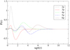 |
Fig. 1. Al I Dirac-Fock radial orbitals for the p symmetry, as a function of |

Each MCDHF calculation was followed by an RCI calculation for an extended expansion, obtained by single, double, and triple (SDT) substitutions from the valence orbitals. As a final step, an RCI calculation was performed for the largest SDT valence expansion augmented by a core-valence (CV) expansion. The CV expansion was obtained by allowing SD substitutions from the valence orbitals and the 2p6 core, with the restriction that there will be at most one substitution from 2p6. All the RCI calculations included the Breit interaction and the leading QED effects. Accounting for CV correlation does not lower the total energies significantly, but it can have large effects on the energy separations and thus we considered it crucial. Core-valence correlation is also important for transition properties (Hibbert 1989). Core-core (CC) correlation, obtained by allowing double excitations from the core, is known to be less important and has not been considered in the present work. The number of CSFs in the final even and odd state expansions, accounting for both VV and CV electron correlation, were 4 362 628 and 2 889 385, respectively, distributed over the different J symmetries.
3.2. Al II
In the singly ionized aluminium, the calculations were more extended, including 78 targeted states. These states belong to the 3s2 ground configuration, and to the 3p2; the 3sns configurations with n = 4, ..., 7; the 3snd with n = 3, ..., 6; and the 3s5g and 3s6g configurations, characterized by even parity, and on the other hand, the 3snp configurations with n = 3, ..., 7; the 3snf with n = 4, 5, 6; and the 3s6h and 3p3d configurations, characterized by odd parity. These configurations define the multireference (MR). In the computations of Al II, the EOL scheme was applied and the CSF expansions were obtained following the active set (AS) approach, accounting for VV and CV correlation. Al II is less complex and the CSF expansions generated from (SD) substitutions are not as large as those in Al I. Hence, we can afford both 2s and 2p orbitals to account for CV correlation. The 1s core orbital remained closed and, as it was for Al I, core-core correlation was neglected. The MCDHF calculations were performed in a similar way to the calculations in Al I, yet no particular restrictions were imposed on the VV substitutions. We optimized six correlation layers corresponding to the 13s, 13p, 12d, 12f, 12g, 8h, and 7i set of orbitals. Each MCDHF calculation was followed by an RCI calculation. Finally, an RCI calculation was performed for the largest SD valence expansion augmented by the CV expansion. The number of CSFs in the final even and odd state expansions, accounting for both VV and CV electron correlation, were 911 795 and 1 269 797, respectively, distributed over the different J symmetries.
4. Results
4.1. Al I
In Table 1 the computed excitation energies, based on VV correlation, are given as a function of the increasing active set of orbitals. After adding the n = 11 correlation layer, we note that the energy values for all 28 targeted states have converged. For comparison, in the second last column the observed energies from the National Institute of Standards and Technology (NIST) Atomic Spectra Database (Kramida et al. 2018) are displayed. All energies but those belonging to the 3s3p2 configuration are already in good agreement with the NIST recommended values. The relative differences between theory and experiment for all three levels of the quartet 3s3p24P state is 3.1%, while the mean relative difference for the rest of the states is less than 0.2%. In the third last column, the computed excitation energies after accounting for CV correlation are displayed. When taking into account CV effects the agreement with the observed values is better overall. Most importantly, for the 3s3p24P levels the relative differences between observed and computed values decrease to less than 0.6%. The likelihood that the 1s22s22p6 core overlaps with the 3s3p2 cloud of electrons is much less than that for 3s2nl. Consequently, when CV correlation is taken into account the lowering of the 3s3p2 energy levels is much smaller than for levels belonging to any 3s2nl configuration. Thus, the adjustments to the separation energies will be minor between the ground state 3s23p and 3s2nl levels, but significant between the 3s23p and 3s3p2 levels. In the last column of Table 1 the differences ΔE = Eobs − Etheor, between the final (CV) computed and the observed energies, are also displayed. In principle, there are two groups of values; the one consisting of the 3s2nd configurations exhibits the smallest absolute discrepancies from the observed energies. For the rest, the absolute discrepancies are somewhat larger.
Computed excitation energies in cm−1 for the 28 lowest states in Al I.
In the calculations, the labelling of the eigenstates is determined by the CSF with the largest coefficient in the expansion of Eq. (2). When the same label is assigned to different eigenstates, a detailed analysis can be performed by displaying their LS-compositions. In Table 1, we note that two of the states have been assigned the same label, i.e. 3s24d 2D, and thus the subscripts a and b are used to distinguish them. In Table 2, we give the LS-composition of all computed 3s2nd 2D states, including the three most dominant CSFs. The 3s24d 2D term appears twice as the CSF with the largest LS-composition. Moreover, the admixture of the 3s3p22D in the four lowest 3s2nd 2D states is rather strong and adds up to 65%. That being so, the 3s3p22D does not exist in the calculated spectrum as a localized state. For comparison, in the last column of Table 2 the labelling of the observed 3s2nd 2D states is also given. In the observed configurations presented by NIST (Kramida et al. 2018), the second highest 3s2nd 2D term has not been given any specific label and it is therefore designated as y2D. The higher 2D terms are designated as 3s24d, 3s25d, and so on.
In Table 3, the current results for the lowest excitation energies are compared with the values from the MCHF-BP calculations by Froese Fischer et al. (2006). The latter calculations are extended up to levels corresponding to the doublet 3s24p 2P state. The differences ΔE between observed and computed energies are given in the last two columns for the different computational approaches. As can be seen, when using the current MCDHF and RCI method the agreement with the observed energies is substantially improved for all levels and in particular, for those belonging to the quartet 3s3p24P state. In the MCHF-BP calculations, core-valence correlation was neglected. As mentioned above and also acknowledged by Froese Fischer et al. (2006), capturing such correlation effects is crucial for 3s-hole states, such as states with significant 3s3p2 composition. Furthermore, the ΔEMCHF − BP values do not always have the same sign, while the ΔERCI differences are consistently positive. This is particularly important when calculating transition properties. On average, properties for transitions between two levels for which the differences ΔEMCHF − BP have opposite signs are estimated less accurately.
Observed and computed excitation energies in cm−1 for the 10 and 20 lowest states in Al I and Al II, respectively.
The complete transition data tables, for all computed E1 transitions in Al I, can be found at the CDS. In the CDS table, the transition energies, wavelengths and the length form of the transition rates A, and weighted oscillator strengths gf are given. Based on the agreement between the length and velocity forms of the computed transition rates ARCI, a statistical analysis of the uncertainties can be preformed. The transitions were arranged in four groups based on the magnitude of the ARCI values. The first two groups contain all the weak transitions with transition rates up to A = 106 s−1, while the next two groups contain the strong transitions with A > 106 s−1. In Table 4, the average value of the uncertainties ⟨dT⟩ (see Eq. (4)) is given for each group of transitions. To better understand how the individual uncertainties dT are distributed, the maximum value and the value Q3 containing 75% of the lowest computed dT values (third quartile) are also given in Table 4. When examining the predicted uncertainties of the individual groups, we deduce that for all the strong transitions dT always remains below 15%. Most of the strong transitions are associated with small uncertainties, which justifies the low average values. Contrary to the strong transitions, the weaker transitions are associated with considerably larger uncertainties. This is even more pronounced for the first group of transitions where A is less than 105 s−1. The weak E1 transitions are challenging, and therefore interesting, from a theoretical point of view, although they are less likely to be observed. The computation of transition properties in the system of Al I is overall far from trivial due to the extreme mixing of the 3s2nd 2D series. Transitions involving any 2D state as upper or lower level appear to be associated with large uncertainties. However, the predicted energy separations are in excellent agreement with observations, meaning that the LS-composition of the 3s2nd 2D states is well described. This should serve as a quality indicator of the computed transition data.
Statistical analysis of the uncertainties of the computed transition rates in Al I and Al II.
Transition rates Aobs evaluated from experimental measurements are compared with the current RCI theoretical values (see Table 5) and with values from the MCHF-BP calculations by Froese Fischer et al. (2006) and the close coupling (CC) calculations by Mendoza et al. (1995). Even though the measurements by Davidson et al. (1990) are more recent than the compiled values by Wiese & Martin (1980), the latter seem to be in better overall agreement with the transition rates predicted by the RCI calculations. In all cases the ARCI values fall into the range of the estimated uncertainties by Wiese & Martin (1980). The only exceptions are the transitions with 3s24d 2D3/2,5/2 a as upper levels, for which the ARCI values agree better with the ones suggested by Davidson et al. (1990). Although the evaluated transition rates by Vujnović et al. (2002) slightly differ from the other observations, they are still in fairly good agreement with the present work. For the  → 3s24s 2S1/2 and
  transitions, the values by Vujnović et al. (2002) are better reproduced by the AMCHF − BP results, yet not enough correlation is included in the calculations by Froese Fischer et al. (2006) and the transition rates predicted by the RCI calculations should be considered more accurate. Whenever values from the close coupling (CC) calculations are presented to complement the MCHF-BP results, the ARCI values appear to be in better agreement with the experimental values. Exceptionally, for the
  transitions, the ACC values by Mendoza et al. (1995) approach the corresponding experimental values more closely. Even so, the ARCI values are still within the given experimental uncertainties. One should bear in mind that according to the estimation of uncertainties by Kelleher & Podobedova (2008b) the ACC values carry relative uncertainties up to 30%. On the contrary, based on the agreement between length and velocity forms, the estimated uncertainties of the current RCI calculations for the above-mentioned transitions are of the order of 3% percent. Therefore, we suggest that the current transition rates are used as a reference.
Comparison between computed and observed transition rates A in s−1 for selected transitions in Al I.
From the computed E1 transition rates, the lifetimes of the excited states are estimated. Transition data for transitions other than E1 have not been computed in this work since the contributions to the lifetimes from magnetic or higher electric multipoles are expected to be negligible. In Table 6 the currently computed lifetimes are given in both length τl and velocity τυ forms. The agreement between these two forms probes the level of accuracy of the calculations. Because of the poor agreement between the length and velocity form of the quartet 3s3p24P and doublet 3s26p 2P states, the average relative difference appears overall to be ∼8%. The differences between the length and velocity gauges of the quartet 3s3p24P states are of the order of 25% on average. These long-lived states are associated with weak transitions and computations involving such transitions are, as mentioned above, rather challenging. In addition, we note that the relative differences corresponding to the 3s26p 2P states exceed 40%. As the computations involve Rydberg series, states between the lowest and highest computed levels might not occupy the same region in space. Nevertheless, these states are part of the same multireference (MR). The highest computed levels correspond to configurations with orbitals up to n = 6, such as 3s26p. To obtain a better description of these levels it is probably necessary to perform initial calculations including in the MR 3s2nl configurations with n = 7 and perhaps even n = 8. This would lead to a more complete and balanced orbital set (Pehlivan Rhodin et al. 2017). When excluding the above-mentioned states, the mean relative difference between τl and τυ is ∼3%, which is satisfactory.
Comparison between computed and observed lifetimes τ in seconds for the 26 lowest excited states in Al I.
In Table 6, the lifetimes from the current RCI calculations are compared with results from the MCHF-BP calculations by Froese Fischer et al. (2006) and observations. Only for the 3s24p 2P state are separated observed values of the lifetimes given for the two fine-structure components. For the rest of the measured lifetimes, a single value for the two fine-structure levels is provided. As can be seen, the overall agreement between the theoretical and the measured lifetimes τobs is rather good. However, the measured lifetimes are better represented by the current RCI results than by the MCHF-BP values. For most of the states, the differences between the RCI and MCHF-BP values are small, except for the levels of the quartet 3s3p24P state. For these long-lived states, no experimental lifetimes exist for comparison.
4.2. Al II
In Table A.1, the computed excitation energies, based on VV correlation, are given as a function of the increasing active set of orbitals. When adding the n = 12 correlation layer, the values for all computed energy separations have converged. The agreement with the NIST observed energies (Kramida et al. 2018) is, at this point, fairly good. The mean relative difference between theory and experiment is of the order of 1.2%. However, when accounting for CV correlation, the agreement with the observed values is significantly improved, resulting in a mean relative difference being less than 0.2%. Accounting for CV effects also results in a labelling of the eigenstates that matches observations. For instance, when only VV correlation is taken into account, the 3F triplet with the highest energy is labelled as a 3s6f level. After taking CV effects into account, the eigenstates of this triplet are assigned the 3p3d configuration, now the one with the largest expansion coefficient, which agrees with observations. There are no experimental excitation energies for the singlet and triplet 3s6h 1, 3H terms. In the last column of Table A.1, the differences ΔE between computed and observed energies are displayed. All ΔE values maintain the same sign, being negative.
In Table 3, a comparison between the present computed excitation energies and those from the MCHF-BP calculations by Froese Fischer et al. (2006) is also performed for Al II. The latter spectrum calculations are extended up to levels corresponding to the singlet 3p21S state and all types of correlation, i.e. VV, CV, and CC, were accounted for. Both computational approaches are highly accurate, yet the majority of the levels is better represented by the current RCI results. The average relative difference for the RCI values is ∼0.2% and for the MCHF-BP ∼0.3%. Moreover, the ΔEMCHF − BP values do not always maintain the same sign, while the ΔERCI values do. Hence, in general, the MCHF-BP calculations do not predict the transition energies as precisely as the present RCI method.
For all computed E1 transitions in Al II, transition data tables can also be found at the CDS. In Table 4, a statistical analysis of the uncertainties to the computed transition rates ARCI is performed in a similar way to that for Al I. The transitions are also arranged here in four groups. Following the conclusions by Pehlivan Rhodin et al. (2017) and Pehlivan Rhodin (2018), the transitions involving any of the 3s7p 1, 3P states have been excluded from this analysis. The discrepancies between the length and velocity forms for transitions including the 3s7p 1, 3P states are consistently large, and thus the computed transition rates are not trustworthy. We note that overall the average uncertainty, as well as the value that includes 75% of the data, appear to be smaller, for each group of transitions, than the predicted values in Al I. Nevertheless, the maximum values of the uncertainties for the last two groups are larger in comparison to Al I. This is due to some transitions involving 3p3d 3F as the upper level. The strong mixing between the 3p3d 3F and the 3s6f 3F levels results in strong cancellation effects. Such effects often hamper the accuracy of the computed transition data and result in large discrepancies between the length and velocity forms.
In Table 7, current RCI theoretical transition rates are compared with the values from the MCHF-BP calculations by Froese Fischer et al. (2006) and, whenever available, results from the B-spline configuration interaction (BSCI) calculations by Chang & Fang (1995). For the majority of the transitions, there is an excellent agreement between the RCI and MCHF-BP values with the relative difference being less than 1%. Some of the largest discrepancies are observed for the 3s3d, 3p21D → 3s3p 1, 3Po transitions. According to Froese Fischer et al. (2006), correlation is extremely important for transitions from such 1D states. In the MCHF-BP calculations, all three types of correlation, i.e. VV, CV, and CC, have been accounted for; however, the CSF expansions obtained from SD-substitutions are not as large as in the present calculations and the LS-composition of the configurations might not be predicted as accurately. Hence, the evaluation of line strengths for transitions involving 1D states and in turn the computation of transition rates involving these states will be affected. Computed transition rates using the BSCI approach are provided for transitions that involve only singlet states. The BSCI calculations do not account for the relativistic interaction and no separate values are given for the different fine-structure components of triplet states. For the 3p21D → 3s3p 1Po transition, the discrepancy between the RCI and BSCI values is also quite large. On the other hand, for the 3s3d 1D → 3s3p 1Po transition, the BSCI result is in perfect agreement with the present ARCI value. The agreement between the current RCI and BSCI transition rates exhibits a broad variation. The advantage of the BSCI approach is that it takes into account the effect of the positive-energy continuum orbitals in an explicit manner. Nevertheless, the parametrized model potential that is being used in the work by Chang & Fang (1995) is not sufficient to describe states that are strongly mixed. Finally, we note the discrepancy for the 3s4p 1Po → 3s21S0 transition, which is quite large between the RCI and MCHF-BP values and inexplicably large between the RCI and BSCI values.
Comparison between computed and observed transition rates A in s−1 for selected transitions in Al II.
In singly ionized aluminium, measurements of transition properties are available only for a few transitions. In Table 7, the available experimental results are compared with the theoretical results from the current RCI calculations, and with the former calculations by Froese Fischer et al. (2006) and Chang & Fang (1995). Transition rates have been experimentally observed for the  transitions in the works by Kernahan et al. (1979), Smith (1970), Berry et al. (1970) and Head et al. (1976), and by Träbert et al. (1999) and Johnson et al. (1986), respectively. In Table 7, the average value of these works is displayed. The agreement with the current RCI results is fairly good. Nonetheless, the averaged Aobs by Träbert et al. (1999) and Johnson et al. (1986) is in better agreement with the value by Froese Fischer et al. (2006). Additionally, Vujnović et al. (2002) provided experimental transition rates for the 3p21D2 → 3s3p 1P1 and 3p21D2 → 3s3p 3P1, 2 transitions by measuring relative intensities of spectral lines. These experimental results, however, differ from the theoretical values.
In the last portion of Table 7, current rates for transitions between states with higher energies are compared with the results from the close coupling (CC) calculations by Butler et al. (1993) and the early results from the configuration interaction (CI) calculations by Chang & Wang (1987). The results from the latter two calculations are found to be in very good agreement. Furthermore, the agreement between the RCI results and those from the CC and CI calculations is also very good for the 3s4f 3F → 3s3d 3D transitions and fairly good for the 3s5f 3F → 3s3d 3D transitions. On the other hand, for the 3p3d, 3s6f 3F → 3s3d 3D transitions, the observed discrepancy between the current RCI values and those from the two previous calculations is substantial. This outcome indicates that the calculations by Butler et al. (1993) and Chang & Wang (1987) are insufficient to properly account for correlation and further emphasizes the quality of the present work.
In the same way as for Al I, the lifetimes of Al II excited states were also estimated based on the computed E1 transitions. In Table A.2, both length τl and velocity τυ forms of the currently computed lifetimes are displayed. As already mentioned, the agreement between these two forms serves as an indication of the quality of the results. The average relative difference between the two forms is ∼2%. The largest discrepancies are observed between the length and velocity gauges of the singlet 3p21D state, and between the singlet and triplet 3s7p 1, 3P states. The highest computed levels in the calculations of Al II correspond to configuration states with orbitals up to n = 7, such as 3s7p. Similarly to the conclusions for the lifetimes of Al I, better agreement between the length and velocity forms of the 3s7p 1, 3P states could probably be obtained by including 3snl configurations with n > 7 in the MR.
In Table A.2, the lifetimes from the current RCI calculations are compared with results from previous MCHF-BP and BSCI calculations by Froese Fischer et al. (2006) and Chang & Fang (1995), respectively. Except for the lifetimes of the triplet 3s3p  and singlet 3p21D2 states, the agreement between the RCI and MCHF-BP calculations is very good. Furthermore, the overall agreement between the RCI and BSCI calculations is sufficiently good. Despite the poor agreement between the RCI and BSCI values for the 3p21D2 and 3s7p 1, 3P states, for the rest of the states the discrepancies are small. The BSCI results are more extended. However, no separate values are provided for the different LSJ-components of the triplet states and the average lifetime is presented for them instead.
In Table A.2, the theoretical lifetimes are also compared with available measurements. The measured lifetime of the 3s3p  state by Träbert et al. (1999) and Johnson et al. (1986) agrees remarkably well with the calculated value by Froese Fischer et al. (2006). The agreement with the current results is fairly good too. The lifetime of the 3s3p
  state measured by Kernahan et al. (1979), Head et al. (1976), Berry et al. (1970), and Smith (1970) is well represented by all theoretical values. On the other hand, the results from the measurements of the 3snf 3F states by Andersen et al. (1971) differ substantially from the theoretical RCI values. For the 3snf 3F Rydberg series, only theoretical lifetimes using the current MCDHF and RCI approach are available. Given the large uncertainties associated with early beam-foil measurements, the discrepancies between theoretical and experimental values are in some way expected. The only exception is the lifetime of the 3s5f 3F state, which is in rather good agreement with the RCI values. In the experiments by Andersen et al. (1971) the different fine-structure components have not been separated and a single value is provided for all three different LSJ-levels.
5. Summary and conclusions
In the present work, updated and extended transition data and lifetimes are made available for both Al I and Al II. The computations of transition properties in these two systems are challenging mainly due to the strong two-electron interaction between the 3s3d 1D and 3p21D states, which dominates the lowest part of their spectra. Thus, some of the states are strongly mixed and highly correlated wave functions are needed to accurately predict their LS-composition. We are confident that in this work enough correlation has been included to affirm the reliability of the results. The predicted excitation energies are in excellent agreement with the experimental data provided by the NIST database, which is a good indicator of the quality of the produced transition data and lifetimes.
We have performed an extensive comparison of the computed transition rates and lifetimes with the most recent theoretical and experimental results. There is a significant improvement in accuracy, in particular for the more complex system of neutral Al I. The computed lifetimes of Al I are in very good agreement with the measured lifetimes in high-precision laser spectroscopy experiments. The same holds for the measured lifetimes of Al II in ion storage rings. The present calculations are extended to higher energies and many of the computed transitions fall in the infrared spectral region. The new generation of telescopes are designed for this region and these transition data are of high importance. The objective of this work is to make available atomic data that could be used to improve the interpretation of abundances in stars. Lists of trustworthy elemental abundances will permit the tracing of stellar evolution, as well as the formation and chemical evolution of the Milky Way.
The agreement between the length and velocity gauges of the transition operator serves as a criterion for the quality of the transition data and for the lifetimes. For most of the strong transitions in both Al I and Al II, the agreement between the two gauges is very good. For transitions involving states with the highest n quantum number for the s and p symmetries, we observe that the agreement between the length and velocity forms is not as good. This becomes more evident when estimating lifetimes of excited levels that are associated with those transitions.
Acknowledgments
The authors have been supported by the Swedish Research Council (VR) under contract 2015-04842. The authors acknowledge H. Hartman, Malmö University, and H. Jönsson, Lund University, for discussions.
References
- Adibekyan, V. Z., Sousa, S. G., Santos, N. C., et al. 2012, A&A, 545, A32 [NASA ADS] [CrossRef] [EDP Sciences] [Google Scholar]
- Andersen, T., Roberts, J. R., & Sørensen, G. 1971, Phys. Scr., 4, 52 [NASA ADS] [CrossRef] [Google Scholar]
- Bensby, T., Feltzing, S., & Oey, M. S. 2014, A&A, 562, A71 [NASA ADS] [CrossRef] [EDP Sciences] [Google Scholar]
- Berry, H. G., Bromander, J., & Buchta, R. 1970, Phys. Scr., 1, 181 [NASA ADS] [CrossRef] [Google Scholar]
- Butler, K., Mendoza, C., & Zeippen, C. 1993, J. Phys. B, 26, 4409 [NASA ADS] [CrossRef] [Google Scholar]
- Buurman, E., & Dönszelmann, A. 1990, A&A, 227, 289 [NASA ADS] [Google Scholar]
- Buurman, E., Dönszelmann, A., Hansen, J. E., & Snoek, C. 1986, A&A, 164, 224 [NASA ADS] [Google Scholar]
- Carretta, E., Bragaglia, A., Gratton, R. G., et al. 2010, A&A, 516, A55 [NASA ADS] [CrossRef] [EDP Sciences] [Google Scholar]
- Chang, T. N., & Fang, T. K. 1995, Phys. Rev. A, 52, 2638 [NASA ADS] [CrossRef] [Google Scholar]
- Chang, T. N., & Wang, R. 1987, Phys. Rev. A, 36, 3535 [NASA ADS] [CrossRef] [Google Scholar]
- Clayton, D. D. 2003, Handbook of Isotopes in the Cosmos: Hydrogen to Gallium (Cambridge: Cambridge University Press) [Google Scholar]
- Davidson, M. D., Volten, H., & Dönszelmann, A. 1990, A&A, 238, 452 [NASA ADS] [Google Scholar]
- Dyall, K. G., Grant, I. P., Johnson, C., Parpia, F. A., & Plummer, E. P. 1989, Comput. Phys. Commun., 55, 425 [NASA ADS] [CrossRef] [Google Scholar]
- Ekman, J., Godefroid, M., & Hartman, H. 2014, Atoms, 2, 215 [NASA ADS] [CrossRef] [Google Scholar]
- Froese Fischer, C. 2009, Phys. Scr., T134, 014019 [Google Scholar]
- Froese Fischer, C., Tachiev, G., & Irimia, A. 2006, At. Data Nucl. Data Tables, 92, 607 [NASA ADS] [CrossRef] [Google Scholar]
- Froese Fischer, C., Godefroid, M., Brage, T., Jönsson, P., & Gaigalas, G. 2016, J. Phys. B: At. Mol. Opt. Phys., 49, 182004 [NASA ADS] [CrossRef] [Google Scholar]
- Gaigalas, G., Rudzikas, Z., & Froese Fischer, C. 1997, J. Phys. B: At. Mol. Opt. Phys., 30, 3747 [Google Scholar]
- Gaigalas, G., Fritzsche, S., & Grant, I. P. 2001, Comput. Phys. Commun., 139, 263 [NASA ADS] [CrossRef] [Google Scholar]
- Gaigalas, G., Zalandauskas, T., & Rudzikas, Z. 2003, At. Data Nucl. Data Tables, 84, 99 [NASA ADS] [CrossRef] [Google Scholar]
- Gaigalas, G., Zalandauskas, T., & Fritzsche, S. 2004, Comput. Phys. Commun., 157, 239 [NASA ADS] [CrossRef] [Google Scholar]
- Gaigalas, G., Froese Fischer, C., Rynkun, P., & Jönsson, P. 2017, Atoms, 5, 6 [NASA ADS] [CrossRef] [Google Scholar]
- Gehren, T., Liang, Y. C., Shi, J. R., Zhang, H. W., & Zhao, G. 2004, A&A, 413, 1045 [NASA ADS] [CrossRef] [EDP Sciences] [Google Scholar]
- Gehren, T., Shi, J. R., Zhang, H. W., Zhao, G., & Korn, A. J. 2006, A&A, 451, 1065 [NASA ADS] [CrossRef] [EDP Sciences] [Google Scholar]
- Grant, I. P. 1974, J. Phys. B, 7, 1458 [Google Scholar]
- Grant, I. P. 2007, Relativistic Quantum Theory of Atoms and Molecules (New York: Springer) [CrossRef] [Google Scholar]
- Head, M. E. M., Head, C. E., & Lawrence, J. N. 1976, in Atomic Structure and Lifetimes, eds. F. A. Sellin, & D. J. Pegg (NY: Plenum), 147 [Google Scholar]
- Hibbert, A. 1989, Phys. Scr., 39, 574 [NASA ADS] [CrossRef] [Google Scholar]
- Jönsson, G., & Lundberg, H. 1983, Z. Phys. A, 313, 151 [NASA ADS] [CrossRef] [Google Scholar]
- Johnson, B. C., Smith, P. L., & Parkinson, W. H. 1986, ApJ, 308, 1013 [NASA ADS] [CrossRef] [Google Scholar]
- Jönsson, G., Kröll, S., Persson, A., & Svanberg, S. 1984, Phys. Rev. A, 30, 2429 [NASA ADS] [CrossRef] [Google Scholar]
- Jönsson, P., Gaigalas, G., Bieroń, J., Froese Fischer, C., & Grant, I. P. 2013, Phys. Commun., 184, 2197 [CrossRef] [Google Scholar]
- Kelleher, D. E., & Podobedova, L. I. 2008a, J. Phys. Chem. Ref. Data, 37, 709 [NASA ADS] [CrossRef] [Google Scholar]
- Kelleher, D. E., & Podobedova, L. I. 2008b, J. Phys. Chem. Ref. Data, 37, 267 [NASA ADS] [CrossRef] [Google Scholar]
- Kernahan, J. A., Pinnington, E. H., O’Neill, J. A. M., Brooks, R. L., & Donnely, K. E. 1979, Phys. Scrip., 19, 267 [NASA ADS] [CrossRef] [Google Scholar]
- Kramida, A., Ralchenko, Y. u., & Reader, J. NIST ASD Team 2018, NIST Atomic Spectra Database, ver. 5.5.3 (Online), available: https://physics.nist.gov/asd (2018, March 15), National Institute of Standards and Technology, Gaithersburg, MD [Google Scholar]
- Lin, C. D. 1974, ApJ, 187, 385 [NASA ADS] [CrossRef] [Google Scholar]
- McKenzie, B. J., Grant, I. P., & Norrington, P. H. 1980, Comput. Phys. Commun., 21, 233 [NASA ADS] [CrossRef] [Google Scholar]
- Mendoza, C., Eissner, W., Le Dourneuf, M., & Zeippen, C. J. 1995, J. Phys. B, 28, 3485 [NASA ADS] [CrossRef] [Google Scholar]
- Mishenina, T. V., Soubiran, C., Bienaymé, O., et al. 2008, A&A, 489, 923 [NASA ADS] [CrossRef] [EDP Sciences] [Google Scholar]
- Nordlander, T., & Lind, K. 2017, A&A, 607, A75 [NASA ADS] [CrossRef] [EDP Sciences] [Google Scholar]
- Olsen, J., Roos, B. O., Jorgensen, P., Jensen, H. J. A. a. 1988, J. Chem. Phys., 89, 2185 [NASA ADS] [CrossRef] [Google Scholar]
- Pehlivan Rhodin, A., Hartman, H., Nilsson, H., & Jönsson, P. 2017, A&A, 598, A102 [NASA ADS] [CrossRef] [EDP Sciences] [Google Scholar]
- Pehlivan Rhodin, A. 2018, Ph. D. Thesis, Lund Observatory [Google Scholar]
- Reddy, B. E., Lambert, D. L., & Allende Prieto, C. 2006, MNRAS, 367, 1329 [NASA ADS] [CrossRef] [Google Scholar]
- Smiljanic, R., Korn, A. J., Bergemann, M., Frasca, A., et al. 2014, A&A, 570, A122 [NASA ADS] [CrossRef] [EDP Sciences] [Google Scholar]
- Smiljanic, R., Romano, D., Bragaglia, A., Donati, P., et al. 2016, A&A, 589, A115 [NASA ADS] [CrossRef] [EDP Sciences] [Google Scholar]
- Smith, W. H. 1970, NIM, 90, 115 [CrossRef] [Google Scholar]
- Sturesson, L., Jönsson, P., & Fischer, C. F. 2007, Comput. Phys. Commun., 177, 539 [NASA ADS] [CrossRef] [Google Scholar]
- Tayal, S. S., & Hibbert, A. 1984, J. Phys. B, 17, 3835 [NASA ADS] [CrossRef] [Google Scholar]
- Taylor, P. R. C. W., Bauschlicher, J., & Langhoff, S. 1988, J. Phys. B, 21, L333 [CrossRef] [Google Scholar]
- Theodosiou, C. E. 1992, Phys. Rev. A, 45, 7756 [NASA ADS] [CrossRef] [Google Scholar]
- Trefftz, E. 1988, J. Phys. B: At. Mol. Opt. Phys., 21, 1761 [NASA ADS] [CrossRef] [Google Scholar]
- Träbert, E., Wolf, A., & Linkemann, J. 1999, J. Phys. B, 32, 637 [Google Scholar]
- Vujnović, V., Blagoev, K., Fürböck, C., Neger, T., & Jäger, H. 2002, A&A, 338, 704 [NASA ADS] [CrossRef] [EDP Sciences] [Google Scholar]
- Weiss, A. W. 1974, Phys. Rev., 9, 1524 [NASA ADS] [CrossRef] [Google Scholar]
- Wiese, W. L., Smith, M. W., & Miles, B. M. 1969, NSRDS-NBS, 22, 47 [Google Scholar]
- Wiese, W. L., & Martin, G. A. 1980, in Transition Probabilities, Part II, Vol. Natl. Stand. Ref. Data System., (Washington DC), Natl. Bur. Std., 68 [Google Scholar]
Appendix A: Additional tables
Computed excitation energies in cm−1 for the 78 lowest states in Al II.
Comparison between computed and observed lifetimes τ in seconds for 75 excited states in Al II.
All Tables
LS-composition of the computed states belonging to the strongly mixed 3s2nd Rydberg series in Al I.
Observed and computed excitation energies in cm−1 for the 10 and 20 lowest states in Al I and Al II, respectively.
Statistical analysis of the uncertainties of the computed transition rates in Al I and Al II.
Comparison between computed and observed transition rates A in s−1 for selected transitions in Al I.
Comparison between computed and observed lifetimes τ in seconds for the 26 lowest excited states in Al I.
Comparison between computed and observed transition rates A in s−1 for selected transitions in Al II.
Comparison between computed and observed lifetimes τ in seconds for 75 excited states in Al II.
All Figures
|
Fig. 1. Al I Dirac-Fock radial orbitals for the p symmetry, as a function of |
| In the text | |
Current usage metrics show cumulative count of Article Views (full-text article views including HTML views, PDF and ePub downloads, according to the available data) and Abstracts Views on Vision4Press platform.
Data correspond to usage on the plateform after 2015. The current usage metrics is available 48-96 hours after online publication and is updated daily on week days.
Initial download of the metrics may take a while.