| Issue |
A&A
Volume 621, January 2019
|
|
|---|---|---|
| Article Number | A79 | |
| Number of page(s) | 17 | |
| Section | Numerical methods and codes | |
| DOI | https://doi.org/10.1051/0004-6361/201833282 | |
| Published online | 11 January 2019 | |
Telluric correction in the near-infrared: Standard star or synthetic transmission?
1
Instituto de Astrofísica e Ciências do Espaço, Universidade do Porto, CAUP, Rua das Estrelas, 4150-762 Porto, Portugal
e-mail: solene.ulmer-moll@astro.up.pt
2
Departamento de Física e Astronomia, Faculdade de Ciências, Universidade do Porto, Portugal
3
European Southern Observatory, Alonso de Córdova 3107, Vitacura, Santiago, Chile
4
Univ. Grenoble Alpes, CNRS, IPAG, 38000 Grenoble, France
Received:
23
April
2018
Accepted:
10
November
2018
Context. The atmospheric absorption of the Earth is an important limiting factor for ground-based spectroscopic observations and the near-infrared and infrared regions are the most affected. Several software packages that produce a synthetic atmospheric transmission spectrum have been developed to correct for the telluric absorption; these are Molecfit, TelFit, and Transmissions Atmosphériques Personnalisées pour l’AStronomie (TAPAS).
Aims. Our goal is to compare the correction achieved using these three telluric correction packages and the division by a telluric standard star. We want to evaluate the best method to correct near-infrared high-resolution spectra as well as the limitations of each software package and methodology.
Methods. We applied the telluric correction methods to CRIRES archival data taken in the J and K bands. We explored how the achieved correction level varies depending on the atmospheric T-P profile used in the modelling, the depth of the atmospheric lines, and the molecules creating the absorption.
Results. We found that the Molecfit and TelFit corrections lead to smaller residuals for the water lines. The standard star method corrects best the oxygen lines. The Molecfit package and the standard star method corrections result in global offsets always below 0.5% for all lines; the offset is similar with TelFit and TAPAS for the H2O lines and around 1% for the O2 lines. All methods and software packages result in a scatter between 3% and 7% inside the telluric lines. The use of a tailored atmospheric profile for the observatory leads to a scatter two times smaller, and the correction level improves with lower values of precipitable water vapour.
Conclusions. The synthetic transmission methods lead to an improved correction compared to the standard star method for the water lines in the J band with no loss of telescope time, but the oxygen lines were better corrected by the standard star method.
Key words: atmospheric effects / radiative transfer / instrumentation: spectrographs / methods: data analysis / techniques: spectroscopic
© ESO 2019
1. Introduction
In ground-based observations, the light coming from a celestial object is partly or totally absorbed by the Earth’s atmosphere, a phenomenon that is strongly wavelength dependent. Even if the position of an observatory is carefully chosen to minimize the impact of the atmosphere, there is still a need to correct for telluric absorption. In spectroscopic studies, the species present in the atmosphere imprint absorption or emission lines on top of the spectra of the target. In absorption, the telluric lines create what is called the transmission spectrum of the Earth’s atmosphere. The volume mixing ratio of the different molecules as a function of height (that can be understood in terms of density profile) present in the atmosphere and the atmospheric conditions (pressure, temperature) affect the telluric lines in their shape, depth, and position in wavelengths. High winds can shift the telluric features, Figueira et al. (2012) showed that a horizontal wind model can account for some of these shifts and is in agreement with radiosonde measurements. Thus, the transmission spectrum depends strongly on the time and location of the observations. Every molecule contributes differently to the final transmission. For example, H2O leads to an absorption over a very wide wavelength range, spanning the optical, near-infrared, and infrared. This absorption defines the near-infrared bands on which photometry and spectroscopy was performed for many years. The water vapour shows hourly to seasonal variations that are challenging to correct (Adelman et al. 2003;Wood 2003). O2 absorption might be easier to correct because it provides sharp, deep, and well-defined features and the O2 volume mixing ratio is more stable in the atmosphere. O2 bands and individual lines in the optical have been studied for a long time (Wark & Mercer 1965; Caccin et al. 1985). When observations are done through cirrus clouds, the atmospheric transmission is not impacted. Cirrus clouds are thin clouds made of ice crystals and usually found at altitudes higher than 6 km (Wylie et al. 1994). The ice crystals transmit most of the incoming stellar light and do not introduce narrow water features in the transmission spectrum.
A correction of telluric absorption is required when the studies aim at high spectral fidelity; for example it is an essential step to characterize planetary and exoplanetary atmospheres (e.g. Bailey et al. 2007; Cotton et al. 2014; Brogi et al. 2014). Telluric correction has also been studied in the context of exoplanet search through radial velocity (RV) measurements.
Earlier on, the telluric lines started to be used as a wavelength calibration to measure precise radial velocities (Griffin & Griffin 1973). The atmosphere can be considered as a gas cell which imposes its absorption features on the target spectrum. Smith (1982) and Balthasar et al. (1982) used O2 lines as wavelength calibrators and could reach a precision down to 5 m s−1. With UVES data, Snellen (2004) used H2O lines as wavelength reference and reached a precision of 5–10 m s−1.
Figueira et al. (2010a) studied the stability of the telluric lines to serve as a wavelength calibration and found a stability of 10 m s−1 over six years and down to 5 m s−1 over shorter timescales. Figueira et al. (2010b) then used the telluric lines as wavelength reference to obtain a RV precision in the near-infrared of 10 m s−1 with CRIRES data. Using the ammonia gas cell technique as wavelength calibration, Bean et al. (2010) were also able to achieve a RV precision of 5 m s−1 and down to 3 m s−1 on short timescales with CRIRES data.
The achievement of higher RV precision implies more stringent limits on the spectral fidelity. This is particularly true for the visible wavelengths, in which a submetre per second is already achieved today (e.g. Lovis et al. 2006). In the visible wavelengths, Cunha et al. (2014) looked at the impact of micro telluric lines (with a depth up to 2%) and demonstrated that the RV impact of these telluric lines was in the range of 10–20 cm s−1, which is comparable to the RV precision that is expected to be achieved by ESPRESSO (Pepe et al. 2014; González Hernández et al. 2017) and required to detect an Earth-mass planet around a solar-like star. In the near-infrared wavelengths, Figueira et al. (2016) presented calculations of the RV information content and showed that the telluric lines are limiting the achievable RV precision but without quantifying the impact. It was found that the impact on RV precision depended on multiple parameters. Some were rooted in the specifications of the spectrograph, like resolution or line sampling. Others were related to the level or quality of the correction itself. However, the final precision depended on how the telluric and stellar spectra overlapped. This means that even for fixed instrumental properties and correction precision, the achievable RV depends significantly on the stellar type, systemic RV, and v sin i.
The historical method to correct for the telluric absorption is the standard star method, where the spectrum of the target is divided by the spectrum of a fast-rotating hot star (often of type O, B, or A) called a telluric standard star (Vidal-Madjar et al. 1986; Vacca et al. 2003). The high temperature and fast rotation of the standard star lead to a low number of resolved stellar lines, so that its spectrum accurately reproduces the atmospheric transmission spectrum. The remaining stellar features are broadened by stellar rotation contrary to the telluric lines which remain narrower, allowing for an easy identification and second-stage removal. The division by the spectrum of the standard star also removes the blaze effect introduced by the spectrograph grating, but this effect can be removed during the data reduction process by other means. In order to accurately reproduce the atmospheric transmission spectrum, the standard star spectrum needs to be taken close in airmass and in time to the spectrum of the target. For reference, at ESO the telluric reference stars are only considered suitable for correction if and only if taken within 2 h and at an airmass difference of up to 0.2 relative to the target star.
However, there are several fundamental limitations in the telluric correction level that can be achieved with the standard star method. First, stellar features can still be present in the spectrum of the standard star. The time of the observation and the pointing direction between the two observations are not the same, which means the light paths probed in the atmosphere are not the same, and as such the atmosphere imprint on these two observations is different (Lallement et al. 1993; Wood 2003). Bailey et al. (2007) showed that the telluric correction of the spectrum of a Sun-like star with the standard star method can lead to errors up to a few percent for the strong telluric lines, and that these errors can be up to 50% when correcting the observations of CO2 features in the atmosphere of Mars.
The authors also demonstrated that these errors can be reduced when a synthetic spectrum of the telluric transmission, calculated with a radiative transfer model, is used instead of a standard star spectrum. Lallement et al. (1993) performed the first telluric correction with forward modelling for the H2O lines near the sodium doublet at 589.5 nm. Seifahrt et al. (2010) reproduced observed telluric lines with a synthetic transmission spectrum to down to a correction level of around 2%. In the last few years, the telluric correction with synthetic transmission spectrum of the Earth’s atmosphere has been intensively developed. TelFit1(Gullikson et al. 2014), Transmissions Atmosphériques Personnalisées pour l’AStronomie2 (TAPAS; Bertaux et al. 2014), and Molecfit3 (Smette et al. 2015; Kausch et al. 2015) among others (e.g. Rudolf et al. 2016; Villanueva et al. 2018) are publicly available codes or web interfaces to perform telluric correction.
Other techniques that retrieve the telluric spectra directly from the observations (in opposition to forward modelling) have been successful, by making clever use of archival data or the sequence of the observations. Artigau et al. (2014) presented a method based on principal component analysis, which uses a large number of standard star observations to build a library of telluric features. The telluric features in the spectra of interest are matched with those in the library and removed. Astudillo-Defru & Rojo (2013) and Wyttenbach et al. (2015) looked at the variation of the flux with the airmass to identify the telluric lines and build a telluric spectrum from the target observations themselves. By assuming a linear dependence between airmass and telluric absorption on the affected pixels (stable in the rest-frame of the detector), they are able to correct high-resolution spectra and detect the elusive calcium and sodium absorption features (respectively) in exoplanetary atmospheres. Snellen et al. (2008) and Brogi et al. (2012, 2014) had already used a similar approach to detect sodium, carbon monoxide, and water vapour in extrasolar planet atmospheres.
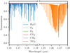 |
Fig. 1. Synthetic transmission spectrum of our atmosphere calculated with the LBLRTM through the TAPAS interface. The main absorber in the first wavelength range is H2O (blue line), while in the second range it is O2 (orange line). The other molecules have a transmission very close to 1. |
On the other hand, Molecfit has been used to search for water vapour on exoplanet atmospheres (Allart et al. 2017) and to study the atmospheric conditions above ESO’s new astronomical site Cerro Amazones (Lakićević et al. 2016). The quest for Earth-like planets around M dwarf drives the development of infrared high-resolution spectrographs. With the arrival of a large number of these spectrographs, such as SPIRou (Moutou et al. 2015), CRIRES+ (Follert et al. 2014), NIRPS (Wildi et al. 2017), and CARMENES (Quirrenbach et al. 2014) among others, the improvement of the ability to perform telluric correction is becoming inevitable.
The different atmospheric models and methodologies should be evaluated in order to understand what is the most efficient way of correcting the absorption introduced by the Earth’s atmosphere. To do so, in the context of RV searches, we used archival CRIRES data and focussed our experiment on a short wavelength domain under well-characterized environmental parameters. In Sect. 2, we introduce the CRIRES data and the reduction process we used. In Sect. 3, we present the three correction methods (Molecfit, TelFit, and TAPAS) and how we implemented the correction procedure in each of them. Section 4 presents the correction done with the standard star method. This section also shows the comparison of the telluric corrections and the impact of airmass and the atmospheric profile on the correction quality. A discussion of the results and the conclusions are presented in Sect. 5.
2. Observations and reduction
To test the telluric correction methods we used near-infrared observations from CRIRES, a high-resolution spectrograph installed at the the Very Large Telescope (VLT) in Paranal. It covers the infrared region from 1.0 to 5.3 μm with a resolving power up to 100 000 depending on the slit being used (Kaeufl et al. 2004). The simultaneous wavelength coverage is however small from λ/70 at 1 μm to λ/50 at 5 μm. We describe below the observations and data reduction.
2.1. Observations
We used archival CRIRES spectra of an M7 V – M8 V dwarf star (Lowrance et al. 2000), HR 7329-B, and a telluric standard of spectral type B9 V (Houk 1978), HIP 100090. According to the CRIRES User Manual version 84.24, the value of the resolution (R) for other slit widths (sw in arcseconds) are derived with the following relation:  . The 0.4” slit width was used, which leads to a resolution around 50 000. The observations were done in two orders. The first order spans from 1.166 μm to 1.188 μm and H2O dominates the telluric absorption in this order. The second order spans from 1.247 μm to 1.272 μm with O2 dominating the telluric absorption in this region. The atmospheric transmission in the wavelength regions we consider is shown in Fig. 1. The observations are listed in Table 1. The spectra were acquired on three consecutive nights from 4 to 6 August 2009 and again from 19 to 21 September 2009 for the two stars, observing the telluric standard less than 2 h after the target star. The signal-to-noise ratio (S/N) is calculated with the Beta Sigma noise estimation from Czesla et al. (2018). We followed their noise estimation on the high-resolution spectrum with several narrow spectral features because this is also the case for our target star and we chose a jump parameter of 2 and an order of approximation of 5.
2.2. Data reduction
The data was reduced using a custom IRAF5 pipeline described in detail in Figueira et al. (2010b). The reduction steps covered are mutual subtraction of eight ABBABBA nodding pairs, linearity correction, and optimal extraction. The extracted spectra are individually continuum normalized, and then co-added to create one spectrum per observation with a higher S/N. An initial wavelength solution is taken from the header keywords provided by the instrument.
3. Telluric correction
TelFit, Molecfit, and TAPAS are three telluric correction methods based on the computation of the atmospheric transmission with the radiative transfer code LBLRTM (Clough & Iacono 1995; Clough et al. 2005). This forward code solves the equation of radiative transfer by calculating the contribution of each line individually. The code uses an atmospheric profile and the line parameters as inputs. The atmospheric profile describes the temperature, pressure and molecule abundances as a function of the altitude. The line parameters include position, intensity, and broadening coefficients taken from the spectroscopic databases HITRAN 2008 (Rothman et al. 2009) and HITRAN 2012 (Rothman et al. 2013).
Details of the observations.
Comparison of the modelling parametrization of the telluric correction methods.
A summary of the capabilities and models employed by each package is shown in Table 2. Appendix A presents the spectra of the telluric standard and the synthetic transmission spectra obtained with each of the packages.
3.1. TelFit
The Python package TelFit (Gullikson et al. 2014) models the atmospheric transmission and fits it to a spectrum with the Levenberg–Marquardt algorithm. TelFit can adjust the wavelength solution of the data to the telluric lines or vice versa with a polynomial function. The order of the polynomial can be set by the user, but the values of the coefficients have to be directly set in the code. TelFit offers a parametric model of the line shape through a Gaussian function and a non-parametric model with the singular value decomposition mode. For each observation, TelFit uses, by default, an average atmospheric profile for mid-latitudes. The website of the Global Data Assimilation System (GDAS)6 enables the use of a custom atmospheric profile, adapted to the location and time of the observations. The GDAS profiles are available for observations taken since 2004 and are updated every three hours.
We used the atmospheric profile that was closest to our observations, with a time difference inferior to 2 h, to first fit the spectrum of the standard star. We experimented with the parametric and non-parametric options for the line shape and attained the same level of correction. Since the other models studied in this work use parametric correction, and to provide a more meaningful comparison, we selected the parametric correction. To perform the fit of the standard star, we left the parameters of the wavelength solution, the continuum level, line shape, resolution, and the mixing ratio of the molecule relevant for the wavelength range considered (H2O or O2) as free parameters.
TelFit does not allow a different parametrization of spectral orders separated by wavelength gaps. Therefore, each of the three CRIRES detectors is treated independently because the parameters of the wavelength solution differ from one detector to the other. As such, for each fit we obtain a different value for the following parameters: molecule abundances, resolution, temperature, and pressure profiles. We homogenize these parameters by taking their mean values weighted by the inverse of the χ2 calculated for each detector. Then, we use the homogenized values of the parameters to compute a final atmospheric transmission for each detector. We divide the stellar spectrum by the atmospheric transmission to correct for the telluric lines. After the correction of the standard star, we use the values of the wavelength solution as the starting values for the fit of the target star and repeat the previous procedure to fit the target’s spectrum.
3.2. Molecfit
Molecfit was developed to correct the telluric lines in the visible and the infrared (Smette et al. 2015; Kausch et al. 2015). It also uses LBLRTM and retrieves automatically the atmospheric profile at the time and place of the observations from an ESO repository updated weekly. However, this repository only contains atmospheric profiles for a limited number of observatories and the user should ask to add a new location.
Similar to TelFit, Molecfit fits a model of the atmospheric transmission to the observed spectrum by adjusting the wavelength solution, continuum level, molecule abundances, and line shape. Molecfit can also adjust the telescope emissivity and considers a larger number of molecules. The telluric lines can be modelled by several functions: Gaussian, Lorentzian, Voigt, or boxcar. Additionally, the so-called expert mode of the package allows for fitting the wavelength and continuum solution independently for each of the CRIRES detectors. Molecfit receives as input a parameter file that describes the parameters to fit and the starting values for each of these. A practical advantage of the expert mode is that it automatically writes a new parameter file with the results from the fit that can be reused as input for a new fit, making it easier to perform iterative fits.
To perform the telluric correction with Molecfit, we used a procedure like that implemented for TelFit. We corrected the standard star spectrum beforehand and then used the wavelength solution in the resulting parameter file as the starting value for the fit of the target. The target spectrum is then fitted twice: First we let free only the parameters of the wavelength solution; in a second step, we leave the molecule abundances as free parameters but we exclude regions of the spectrum that contain stellar lines. Since with expert mode the three detectors are fitted at the same time, we do not need to homogenize any parameters and perform a second fit using these. After the second fit, Molecfit divides the spectrum of the target by the computed atmospheric transmission to correct for the telluric lines.
3.3. TAPAS
The TAPAS web interface is described in Bertaux et al. (2014). It also computes the atmospheric transmission with the LBLRTM. However, the atmospheric profile is derived from the European Centre for Medium-Range Weather Forecasts (ECMW)7, a weather database updated every 6 h. The result of a TAPAS query is the atmospheric transmission spectrum at the time and location of the observations, at a chosen resolution.
There is no fitting procedure included in TAPAS, and thus we had to implement one in order to obtain a telluric correction comparable to TelFit and Molecfit. Since TAPAS allows us to download the contribution of each molecule independently, we chose to scale only the abundance of the main absorber in each order, either O2 or H2O, in order to match the observed spectra. We downloaded two transmission spectra for each observation: one with only the main absorber, called Tm, and another transmission spectra with the absorption by the other molecules (O3, CO2, CH4, N2O and H2O or O2 depending on the order) and the Rayleigh scattering, called Tr. The impact of the Rayleigh scattering on our observations at 1.1 μm is less then 1% of the total transmittance (0.995).
The transmission spectrum can be scaled by scaling the optical depths for optically thin lines as done in Bertaux et al. (2014) and Baker et al. (2017). The total TAPAS transmittance is then given by Ttapas = (Tm)αTm, with α the scaling factor.
In order to correct for the telluric lines, we performed a series of simple fits of the TAPAS transmission spectrum Ttapas to the CRIRES target spectrum Fstar. The fits are carried out with the Scipy function curve_fit using the Levenberg–Marquardt algorithm. The procedure is similar to what is done in TelFit and Molecfit. Since it is well known that the wavelength-calibration solution of high-resolution spectrographs changes from detector to detector, we chose to fit each of these independently.
We performed a wavelength calibration on both the standard star and the target spectra using the TAPAS transmission spectrum. The wavelength solution is fitted with a third degree polynomial a + bλ + cλ2 + dλ3. The starting values for b, c and d in the fit of the standard star are set to 0. The offset a is set to 0.05 to facilitate convergence. The starting values for the target star are the results of the standard star fit.
Then, we fit the continuum of the TAPAS transmission with a second degree polynomial and we scaled the transmission spectrum of the main absorber as detailed above. Since we fit the three detectors independently, we obtained three values for the scaling factor α for one observation. To homogenize the values of the scaling, we calculated their weighted mean using as weights the inverse χ2 of each detector, as was done for the TelFit correction. Once the wavelength solution, continuum, and scaling have been fitted, we divided the science spectrum by the fitted TAPAS transmission to perform the telluric correction.
4. Comparison
We corrected the CRIRES data with TelFit, Molecfit, and TAPAS following the procedures explained in Sect. 3. Since we have standard star observations, we also performed the telluric correction using the standard star method. We shifted the standard star in RV to match the target star using the DopplerShift function from the PyAstronomy package8. We chose the RV shift that minimizes the residuals between the two spectra. Then, we divided the target by the standard star to obtain the telluric-corrected spectrum.
4.1. Examples of correction
Two examples of the level of telluric correction obtained with our dataset are presented in this section. The telluric correction for the whole wavelength range with the four methods is presented in Appendix B. In Fig. 2, we present an example of the telluric correction with Molecfit, on the third detector, for the standard star spectrum. The wavelength range is dominated by H2O absorption and the correction level is high with residuals below 2%. Figure 3 shows the telluric correction of the target spectrum on the same wavelength range. The telluric correction was also performed with Molecfit. The input spectrum is plotted in blue with the error bars, the fitted Molecfit transmission is in red and shows that all the telluric lines are well matched. The telluric lines are corrected at the noise level of the spectrum. In the bottom part, we show the residuals of the difference between the input spectrum and the atmospheric transmission. We identified strong K I stellar lines with the NIST database9 and we excluded these regions in order to calculate the mean and standard deviation of the residuals presented in Figs. 4 and 6. In Figs. 5 and 7 we selected only points inside the telluric lines, thus the broad stellar variations are excluded from the standard deviation measurements.
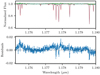 |
Fig. 2. Standard star spectrum corrected with Molecfit. Top panel: input spectrum is indicated in blue, Molecfit atmospheric transmission is indicated in red, corrected spectrum is indicated in green. Bottom panel: residuals obtained after the subtraction of the atmospheric transmission to the input spectrum. |
4.2. H2O absorption
We compare the telluric correction obtained with TelFit, Molecfit, TAPAS, and the standard star method in the wavelength range 1.166–1.188 μm where H2O is the main absorber. Figure 4 presents the mean and standard deviation of the residuals for each of the three observations. Ideally, the offset of the residuals, represented by the mean, should be zero. This is the case for TelFit and Molecfit for the first observation, which has an offset very close to zero. For the two other observations, TelFit and Molecfit have an offset around 0.3% and 0.4%, respectively. The TAPAS package and the standard star method have a higher offset for the first observation of close to 0.2% and a similar offset (around 0.3–0.4%) for observations 2 and 3. A positive mean can indicate that the telluric lines might be under-corrected, meaning the modelled line is not as deep as the line in the input spectrum. The standard deviation of the residuals should also tend to zero, however we are limited here by a large scatter already present in the spectra. The standard deviation of the residuals seems to be only affected by the observation and not by which method is used for the correction.
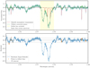 |
Fig. 3. Example of a telluric-corrected spectrum with Molecfit. Top panel: input spectrum of the target star is indicated in blue, Molecfit atmospheric transmission is shown in red, corrected spectrum is shown in green. Excluded stellar lines are shown in light yellow. Bottom panel: residuals between the input spectrum and atmospheric transmission. The dashed lines represent the upper and lower 5% limits. The points that belong to telluric lines and are not blended with stellar lines are identified in orange. |
Figure 5 is similar to the previous figure except with the points inside the telluric lines. Molecfit and TelFit have systematically lower scatter and offset than the standard star method. The Molecfit offset is the closest to zero. Also, TAPAS has a lower scatter than the standard star method, but its offset is higher for observations 2 and 3. The correction with standard star method could be improved by scaling its spectrum in order to adjust the H2O absorption. In this wavelength domain, dominated by water absorption, we conclude that Molecfit, TelFit, and TAPAS give a better telluric correction than the standard star method.
4.3. O2 absorption
We compare the telluric correction obtained with the four methods in the wavelength range 1.247–1.272 μm where O2 is the main absorber. Figures 6 and 7 present the offset and scatter of the residuals for all the points (excluding the K I stellar lines) and for the points inside the telluric lines, respectively. Molecfit and the standard star method clearly give smaller offsets, always below 0.5%, for all observations (Fig. 6). The scatter of the residuals is equivalent for all methods. For the residuals inside the telluric lines (Fig. 7), the smallest offsets are seen with Molecfit and the standard star method. Even though the mean of the Molecfit residuals inside telluric lines is the closest to zero, Molecfit presents a higher scatter inside the telluric lines compared to the standard star method and TAPAS.
The correction of O2 telluric lines is clearly more challenging for TAPAS, Molecfit, and TelFit. These last two packages scale the O2 content in the atmospheric profile, contrary to TAPAS, where we only scale the O2 transmission a posteriori and to the standard method, for which there is no scaling. The O2 absorption at 1.2 μm is composed of several deep and wide features at this resolution, creating a wide absorption band. This band was partly removed by the continuum normalization completed prior to the telluric correction. This could explain why the telluric correction with TAPAS results in offset residuals. For TelFit this explanation is excluded since we did not compute the continuum contribution of the lines with LBLRTM.
4.4. Shape of the O2 lines
The line shape is a fitted parameter for the synthetic transmission method. Molecfit and TelFit have several line profiles available, while TAPAS only has a Gaussian profile. In order to check if the parametrization we used was adequate, we studied the O2 lines imprinted in the standard star spectrum. To do so, we calculated the cross-correlation function (CCF) between the standard star spectrum and a mask of O2 lines. The mask contains 22 lines with an average depth of 0.61. The CCF created by this process has not only a higher S/N, but a much higher sampling than the individual lines present in the original spectra. As such, this CCF allows a finer evaluation of the average profile of telluric lines. To create the mask, we selected the positions of the O2 lines from the HITRAN website10. We calculated the width of the mask in RV as  , where c is the speed of light, R is the resolution, and the factor of 2 comes from the CRIRES sampling. Then, we measured the bisector line of the CCF. The results are plotted in Fig. 8. We calculated the bisector inverse slope for each observation and we found similar values presented in Table 3. The bisectors calculated for each observation are very similar, which means the variations of the line shape between observations is small. Besides, the bisector does not show strong asymmetries, which confirms that the symmetric functions used by Molecfit and TelFit to model the lines are adequate.
4.5. Sensitivity to airmass and relative humidity
The atmospheric and observing conditions, such as airmass and relative humidity, affect the transmission spectrum of the atmosphere. We study how the correction for the atmospheric transmission spectrum is influenced by the airmass and relative humidity values. First, we use the CRIRES data presented in Sect. 2, which spans a small range of airmasses and humidities. We notice a positive correlation between the airmass and the standard deviation of the residuals for all telluric correction methods. For the relative humidity, the smallest residuals are found at the highest humidity value. Thus, the slight change in humidity does not seem to affect our telluric correction.
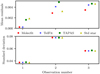 |
Fig. 4. Mean and standard deviation of the residuals of all points except the stellar lines for the four telluric correction methods Molecfit (red circle), TelFit (blue cross), and TAPAS (green square), and the standard star method (yellow triangles) in the wavelength range dominated by H2O absorption. |
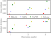 |
Fig. 5. Mean and standard deviation of the residuals inside the telluric lines for the four telluric correction methods in the wavelength range dominated by H2O absorption. The colour code is the same as Fig. 4. |
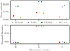 |
Fig. 6. Mean and standard deviation of the residuals of all points except the stellar lines for the four telluric correction methods in the wavelength range dominated by O2 absorption. The colour code is the same as Fig. 4. |
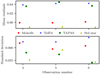 |
Fig. 7. Mean and standard deviation of the residuals inside the telluric lines for the four telluric correction methods in the wavelength range O2 absorption. The colour code is the same as Fig. 4. |
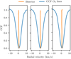 |
Fig. 8. Cross-correlation function (blue line) and its bisector (orange line) of the O2 lines from the standard star spectra for observations 4, 5, and 6. |
To investigate a wider range of these two parameters, we use a second CRIRES dataset. This dataset is composed of seven stars with stellar types ranging from F9 V to K3 V. The 16 spectra are taken in the K band, around 2.15 μm. The observations were carried out between April and August 2012, and cover airmasses from 1.0 to 1.6 and relative humidities from 3% to 33%. We reduced the spectra with the same pipeline used for the first dataset and explained in Sect. 2. Then, we performed the telluric correction of each spectrum with Molecfit, TelFit, and TAPAS. The telluric corrections were done as explained in Sect. 3, but without using a first approximation for the wavelength solution. We made sure to measure the correction level of telluric lines that were not blended with stellar lines.
Bisector inverse slope of the CCF of O2 lines for the three observations.
We show the standard deviation of the residuals, which represents the scatter of the residuals, obtained with the three methods in Fig. 9. Overall, the scatter of the residuals obtained with TAPAS is higher than with Molecfit and TelFit, which confirms the results obtained from the first dataset. For airmasses below 1.3, the scatter is close to 2% for Molecfit and TelFit while the scatter is around 4% for TAPAS. We notice a positive trend of the scatter with airmass for the Molecfit and TelFit points but not for the TAPAS points. In Fig. 10, we show the residuals of Molecfit as functions of airmass, relative humidity, and S/N. The scatter values obtained with Molecfit are similar to those obtained with TelFit. The relative humidity is traced with the colour bar, the vertical gradient from green to blue indicates that the scatter increases with higher values of relative humidity. A positive trend is also noticeable for airmasses higher than 1.4, hence the increasing scatter can be attributed to both parameters. At low airmass, below 1.2, the spectra with higher scatter might be explained by their lower S/N and their relative humidity around 15%. With this larger sample of airmass and relative humidity, we find that both of these parameters have an impact on the correction level which can be obtained. For Molecfit and TelFit telluric corrections, higher values of airmass and relative humidity correlate with higher scatter of the residuals.
4.6. Effect of the atmospheric profile
We investigate the impact of the input atmospheric profile on the telluric correction. An atmospheric profile describes how the pressure and temperature vary with altitude, and the volume mixing ratio of several atmospheric molecules as a function of altitude. First, we describe three MIPAS atmospheric profiles available as inputs for the telluric correction software packages Molecfit and TelFit. Then we compare the telluric correction obtained by the two profiles available for Molecfit because this package offers the most tailored atmospheric profile for the Paranal Observatory.
4.6.1. Different atmospheric profiles
The MIPAS profiles from 2001, created by John Remedios, are available for mid-latitude (45°), for polar latitude (75°), and equatorial latitude. These profiles, available online11, include 30 molecules and 6 others can be included.
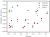 |
Fig. 9. Scatter of the residuals for the three telluric correction methods Molecfit (red circle), TelFit (blue cross), and TAPAS (green square) as a function of airmass. |
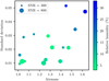 |
Fig. 10. Scatter of the residuals for the telluric correction with Molecfit as functions of airmass (abscissa), relative humidity (colour bar), and S/N (point size). |
The default profile for Molecfit is the equatorial daytime profile. However, Molecfit allows the user to use a tailored profile for the Paranal and La Silla observatories by merging the MIPAS equatorial profile with data from the ESO Meteo Monitor (EMM) and the GDAS profile. The EMM measures the relative humidity, air temperature, pressure, and dew point temperature close to the telescopes, and the GDAS profile describes the atmosphere from 0 to 26 km and is updated every 3 h. For TelFit the default profile is the mid-latitudes at night time profile. TelFit also facilitates the use of a tailored profile, which is the GDAS profile.
We plot in Fig. 11 the equatorial daytime profile, mid-latitude profile, and one of the tailored profiles by Molecfit, called a merged profile. The H2O volume mixing ratio of the merged profile is much lower than the two other profiles up to a certain height (16 km), which reflects the dry condition of the Paranal Observatory. Using the Molecfit merged profile is in this case more adequate to fit the transmission spectrum to the CRIRES data. The merged profile is identical to the equatorial profile above the altitude of 26 km because the GDAS profile does not provide information at an altitude higher than 26 km. The difference between the merged and equatorial are smaller than 10−3 at an altitude higher than 26 km for all plots. Below an altitude of 26km, the difference between the merged and equatorial profile are larger. The median of the difference is equal to 1.9 K for the temperature, 1.2 mbar for the pressure, and 730 ppmv for H2O. For O2, CH4, and O3 the median of the difference is equal to 0. The O2 volume mixing ratio is similar in the three profiles: equatorial, mid-latitudes, and merged profile. The volume mixing ratio of O3 and CH4 in the mid-latitude and equatorial profiles differ but we cannot quantify the differences since O3 and CH4 do not affect the wavelength range of our observations.
Moreover, the concentration of greenhouse gases such as CH4 and CO2 is increasing every year, as shown on the Earth System Research Laboratory website12 with measurements done at Mauna Loa, Hawaii. The concentration of CH4 in 2001 (MIPAS profiles) was 1.771 ppmv and was 1.842 ppmv in 2016, while the concentration of CO2 was equal to 371.1 ppmv in 2001 and increased to 404.21 ppmv in 2016. For that matter the Molecfit User Manual13 recommends increasing the value of CO2 by 6%.
4.6.2. Correction with the equatorial and merged profiles
We corrected the target spectra with Molecfit as described in Sect. 3 using the merged profile (EMM + GDAS + equatorial), the equatorial profile, and the equatorial profile updated with the water volume mixing ratio derived from the standard star. The Molecfit package provides the volume mixing ratio of water in ppmv and the column height of the precipitable water vapour (PWV) in mm. The column height of PWV is the height of liquid water contained in a vertical column above the observing site if the water vapour was condensed (Marvil et al. 2006). The calculation to compute the column height of PWV is presented by Eq. (9) in Smette et al. (2015). We plot in Fig. 12 the resulting values of the H2O column obtained with the three atmospheric profiles. Even though each fit gives a different value, the results are all consistent within their error bars. We notice that the water column derived by Molecfit is increasing with the observation number, contrary to the relative humidity measured at the telescope.
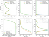 |
Fig. 11. Atmospheric profiles: MIPAS Equatorial in blue, MIPAS mid-latitude daytime in orange, and Molecfit best-fit merged profile in green. The merged profile is composed of the interpolation of the GDAS profiles from 05.08.2008 between 3 h and 6 h, and on-site measurements taken in the header of the spectrum. The relative humidity taken at the telescope is equal to 4%, the pressure to 745 mbar, and the temperature to 286 K. |
We measured the residuals between the input spectrum and the Molecfit transmission spectrum inside the telluric lines uncontaminated by stellar lines. Figure 13 shows the mean and standard deviation of these residuals. The offset and scatter are increasing with the observation number. Hence, there is a correlation between the water column derived by Molecfit and the accuracy of the telluric correction.
A slight difference in water content within the error bars has an impact on the level of the telluric correction. Figure 13 also shows that the merged profile always gives smaller mean residuals than the equatorial profile for the three observations. We notice that when we updated the starting value of H2O (green data), the residuals are closer to those obtained with the merged profile, which denotes the sensitivity of Molecfit to the starting values.
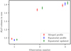 |
Fig. 12. H2O column in mm derived from 3 observations of the target star by Molecfit. The red points are obtained using the merged atmospheric profile; the blue points are obtained using the equatorial atmospheric profile. The fit converged to a zero solution for the second observation. Thus, the green points are obtained with the same equatorial profile as the blue points, but the H2O initial value is modified to that found with the standard star fit. |
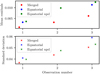 |
Fig. 13. Mean and standard deviation of the residuals inside the telluric lines. The telluric correction was done with Molecfit using three different atmospheric profiles as inputs. The colour code is the same as Fig. 12. |
5. Discussion and conclusions
We performed telluric correction in the near-infrared on CRIRES data with three software packages using a synthetic atmospheric transmission. We also compared these corrections with the standard star method that is commonly used. The standard star method has several disadvantages, such as the time and airmass differences between the target and standard star observations, which result in slightly different atmospheric transmission spectra. Another problem is the loss of telescope time spent observing telluric standard stars. Using synthetic transmission spectra to model the telluric absorption is a good opportunity to correct archival data for which no suitable standard star was observed but also to save observing time.
We chose to study the oxygen and water telluric absorption because these molecules have been used for a long time as wavelength calibrators and have opposite characteristics: the water absorption varies on short timescales and in strength while the oxygen absorption is quite constant in time and in strength. For the wavelength range dominated by water absorption, we found that the synthetic transmission methods deliver a more precise telluric correction. Inside the water telluric lines, the synthetic transmission methods present systematically lower scatter than the standard star method. At most, the standard star method has a scatter 1.3 times larger than Molecfit. We interpret this because water absorption varies quickly in time and the use of a synthetic transmission of the atmosphere allows us to account for these rapid changes better than the standard star method.
We also found that the constant increase in the scatter of the residuals between observation 1, 2, and 3 is correlated with the increase of the PWV derived by Molecfit. Deep and narrow water lines might be more difficult to model if the lines are not well sampled. The correction level obtained with Molecfit using any of the atmospheric profile is still higher than with the standard star method.
For the wavelength range dominated by oxygen absorption the standard star method performs better. The synthetic transmission methods present a scatter up to 1.2 times higher in the residuals than the standard star method. Looking more closely inside the telluric lines, Molecfit presents a higher scatter than the standard method but a smaller offset. The TelFit and TAPAS packages result in a global offset around 1%. For TAPAS, we explain this difference by the fact that part of the O2 absorption was removed at the time of the continuum normalization. Gullikson et al. (2014) also pointed out that TelFit fits with a higher precision the water lines compared to the oxygen lines. They attributed it to a probable systematic error in the line strength in the HITRAN database because two O2 bands were under- and over-fitted by the same mixing ratio at the time. We cannot test this hypothesis because we have only one O2 band. It might be that the spectroscopic parameters of the O2 molecule require some revisions.
Using additional CRIRES observations, which cover a wider range of airmass and relative humidity, we compared the three synthetic transmission methods. We found that Molecfit and TelFit have a smaller scatter than TAPAS, especially at low airmass where the scatter obtained with TAPAS is two times higher. We also showed that an increase in both airmass and relative humidity lead to higher scatter of the residuals for the Molecfit and TelFit methods.
On the use of a tailored atmospheric profile for the observatory site, we showed that the merged atmospheric profile calculated by Molecfit always leads to smaller residuals than the equatorial profile. The merged profile takes into account on-site measurements at Paranal and GDAS atmospheric profiles modelled from a set of meteorological data. The GDAS profiles are available up to an altitude of 26 km and at higher altitude the merged profile uses the equatorial profile. The merged profile provides starting values closer to the solution and helps the fit to converge to a solution with a higher precision.
Of the three packages studied, Molecfit is the most complete package; it allows for correction of the telluric absorption across the largest wavelength domain and with the largest number of variables. The Molecfit method is developed by ESO, it is constantly maintained and, at the time of the writing (November 2018), the latest release is dated from September 2018. The merged atmospheric profile is automatically downloaded and computed by Molecfit. The large number of variables available to fit the telluric spectra might actually be a disadvantage, both for the user and the fitting algorithm. For the user, it might be difficult to pinpoint the right values for each instrument, while the high number of parameters does not help the convergence of the minimization algorithm.
The TelFit package is an easy to use Python code that can quickly be integrated into an existent code. We found that calibrating the wavelength solution to the telluric lines was much harder than with Molecfit and we were not able to perform the wavelength calibration of the data with the telluric lines. In addition, as mentioned in Gullikson et al. (2014), the scaling by TelFit of the molecular mixing ratios does not allow for retrieval of the atmospheric parameters, contrary to Molecfit. The download of the GDAS atmospheric profile is not automated, so we created a script, available online14, to fill the form and download the profile.
The TAPAS package delivers the atmospheric transmission function, which has to be fitted to the data to obtained comparable results to the other methods. The code we wrote to apply this fitting is also available on-line. It was developed to use with CRIRES data, but it can be adapted to be used with other spectrographs. The individual atmospheric transmissions for each molecule are available to download, information that is essential to fit the abundances of the main absorber. The TAPAS method does not require any software installation, only a user account. Disadvantages to TAPAS are that it relies on website availability and that all the fitting process has to be done after the download of the atmospheric transmission. The telluric correction using the TAPAS method would certainly benefit from a fitting procedure being included during the computation of the atmospheric transmission.
On top of the explored software packages, other similar and available tools could have been used to perform the telluric correction. The Tellrem tool uses the same principle as TelFit to compute the atmospheric transmission and to fit the observed spectrum. However, the line shape fitting can only be done with a Gaussian profile of varying width and the wavelength solution is adjusted with a first degree polynomial. Overall, Molecfit and TelFit are very similar to this code; this is one of the reasons we chose not to include Tellrem in the comparison. Also, Tellrem is tailored to be used with X-shooter spectra, however it could be used to correct spectra from other instruments. The installation procedure is more complicated than for the two codes because the different components (radiative transfer code, line database, and atmospheric profiles) all need to be installed separately.
The Planetary Spectrum Generator (PSG; Villanueva et al. 2018) models synthetic planetary spectra from the ultraviolet to the radio wavelengths. To do so, PSG uses several radiative transfer codes and spectroscopic databases. The on-line interface allows for synthesizing the Earth transmittance at the altitude of the Paranal Observatory, which could be used to model the telluric absorption in the CRIRES observations. The user can upload parts of their spectrum on the interface and perform the fitting of the transmission spectrum to the data remotely.
The synthetic atmospheric transmission methods can be limited in case the target star has a lot of intrinsic features, which complicate the fitting of the telluric lines. The fitting of the synthetic transmission spectra to the observed spectra should ideally be carried out in regions where there are no blending between the stellar and telluric lines. The fitting ranges can be small (few tens of angstroms), and stellar lines inside the fitting ranges should be excluded. However, if no individual telluric line can be identified, the best option might be to keep the molecular column densities constant and only adjust the wavelength solution for example. In that case the telluric correction might not lead to the level of correction presented in this work.
The standard star method is a simple and efficient way to correct for the telluric lines, especially in regions where the water absorption is small. However, the synthetic transmission methods offer a good alternative to the loss of telescope time spent to observe standard stars and facilitates obtaining a better precision for the fitting of the water lines. As a future improvement, it would be important to optimize the fitting algorithms (in particular for Molecfit and TelFit) to explore the parameter space in a more efficient way that is not so dependent on the input values. It would also be important to compare the different telluric correction methods on a wider wavelength range, as made available by new generation spectrographs.
Acknowledgments
This work was funded by FEDER – Fundo Europeu de Desenvolvimento Regional funds through the COMPETE 2020 - Programa Operacional Competitividade e Internacionalização (POCI), and by Portuguese funds through FCT – Fundação para a Ciência e a Tecnologia in the framework of the project POCI-01-0145-FEDER-032113. This work was supported by Fundação para a Ciência e a Tecnologia (FCT, Portugal) through national funds and from FEDER through COMPETE2020 by the grants UID/FIS/04434/2013 & POCI-01-0145-FEDER-007672, and PTDC/FIS-AST/1526/2014 & POCI-01-0145-FEDER-016886. N.C.S. acknowledges support by Fundação para a Ciência e a Tecnologia (FCT) through Investigador FCT contract of reference IF/00169/2012/CP0150/CT0002. J.J.N. acknowledges support of the FCT fellowship PD/BD/52700/2014. Plots were done with Matplotlib from Hunter (2007). The authors thank Janis Haldeberg for providing the data and Alain Smette for his help with Molecfit.
Appendix A: Transmission spectra
This appendix presents the three synthetic transmission spectra obtained with Molecfit, TelFit, and TAPAS as well as the standard star spectrum. Figure A.1 shows the wavelength range from 1.166 μm to 1.188 μm, where water absorption dominates. The standard star spectrum has lines remaining that are not matched by the synthetic transmission spectra. The remaining lines at 1.168 μm are probably due to a detector problem since previous spectra of the same star do not show these lines. The line at 1.1867 μm resembles a narrow telluric line, but it is not reproduced by any of the synthetic atmospheric transmission spectra. Figure A.2 shows the second wavelength range from 1.247 μm to 1.272 μm, where oxygen absorption dominates. In this figure, we do not notice remaining lines in the standard star spectrum. The major difference is the continuum level of each synthetic transmission spectra.
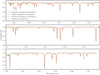 |
Fig. A.1. Synthetic transmission spectra and the standard star spectrum dominated by water absorption. The blue curve is computed with Molecfit, the orange curve with TelFit, the green curve with TAPAS, and the red curve is the standard star spectrum. |
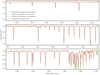 |
Fig. A.2. Synthetic transmission spectra and the standard star spectrum dominated by oxygen absorption. The colour code is same as Fig. A.1. |
Appendix B: Telluric corrections
We present the plots of the telluric correction in both wavelength ranges. The telluric correction was performed with Molecfit in Figs. B.1 and B.5, TelFit in Figs. B.2 and B.6, TAPAS in Figs. B.3 and B.7, and the standard star method in Figs. B.4 and B.8.
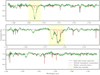 |
Fig. B.1. Example of a telluric-corrected spectrum with Molecfit. The input spectrum is indicated in black, the atmospheric transmission spectrum is indicated in red, and the telluric-corrected spectrum is indicated in green. |
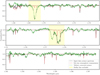 |
Fig. B.4. Example of a telluric-corrected spectrum with the standard star method. The colour code is same as Fig. B.1. |
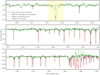 |
Fig. B.5. Example of a telluric-corrected spectrum with Molecfit. The colour code is same as Fig. B.1. |
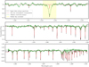 |
Fig. B.8. Example of a telluric-corrected spectrum with the standard star method. The colour code is same as Fig. B.1. |
Pieter Tans, NOAA/ESRL, esrl.noaa.gov/gmd/ccgg/trends
References
- Adelman, S. J., Bikmaev, I., Gulliver, A. F., & Smalley, B. 2003, IAU Symp., 210, 337 [NASA ADS] [Google Scholar]
- Allart, R., Lovis, C., Pino, L., et al. 2017, A&A, 606, A144 [NASA ADS] [CrossRef] [EDP Sciences] [Google Scholar]
- Artigau, E., Astudillo-Defru, N., Delfosse, X., et al. 2014, Proc. SPIE, 9149, 914905 [Google Scholar]
- Astudillo-Defru, N., & Rojo, P. 2013, A&A, 557, A56 [NASA ADS] [CrossRef] [EDP Sciences] [Google Scholar]
- Bailey, J., Simpson, A., & Crisp, D. 2007, PASP, 119, 228 [NASA ADS] [CrossRef] [Google Scholar]
- Baker, A. D., Blake, C. H., & Sliski, D. H. 2017, PASP, 129, 085002 [NASA ADS] [CrossRef] [Google Scholar]
- Balthasar, H., Thiele, U., & Wohl, H. 1982, A&A, 114, 357 [NASA ADS] [Google Scholar]
- Bean, J. L., Seifahrt, A., Hartman, H., et al. 2010, ApJ, 713, 410 [NASA ADS] [CrossRef] [Google Scholar]
- Bertaux, J. L., Lallement, R., Ferron, S., Boonne, C., & Bodichon, R. 2014, A&A, 564, A46 [NASA ADS] [CrossRef] [EDP Sciences] [Google Scholar]
- Brogi, M., Snellen, I. A. G., Kok, D., et al. 2012, Nature, 486, 502 [NASA ADS] [CrossRef] [PubMed] [Google Scholar]
- Brogi, M., de Kok, R.J., Birkby, J. L., et al. 2014, A&A, 565, A124 [NASA ADS] [CrossRef] [EDP Sciences] [Google Scholar]
- Caccin, B., Cavallini, F., Ceppatelli, G., Righini, A., & Sambuco, A. M. 1985, A&A, 149, 357 [NASA ADS] [Google Scholar]
- Clough, S. A., & Iacono, M. J. 1995, J. Geophys. Res., 100, 16519 [NASA ADS] [CrossRef] [Google Scholar]
- Clough, S. A., Shephard, M.W., Mlawer, E. J., et al. 2005, J. Quant. Spectr. Rad. Transf., 91, 233 [NASA ADS] [CrossRef] [MathSciNet] [Google Scholar]
- Cotton, D. V., Bailey, J., & Kedziora-Chudczer, L. 2014, MNRAS, 439, 387 [NASA ADS] [CrossRef] [Google Scholar]
- Cunha, D., Santos, N. C., Figueira, P., et al. 2014, A&A, 568, A35 [NASA ADS] [CrossRef] [EDP Sciences] [Google Scholar]
- Czesla, S., Molle, T., & Schmitt, J. H. M. M. 2018, A&A, 609, A39 [NASA ADS] [CrossRef] [EDP Sciences] [Google Scholar]
- Figueira, P., Pepe, F., Lovis, C., & Mayor, M. 2010a, A&A, 515, A106 [NASA ADS] [CrossRef] [EDP Sciences] [Google Scholar]
- Figueira, P., Pepe, F., Melo, C. H. F., et al. 2010b, A&A, 511, A55 [NASA ADS] [CrossRef] [EDP Sciences] [Google Scholar]
- Figueira, P., Kerber, F., Chacon, A., et al. 2012, MNRAS, 420, 2874 [NASA ADS] [CrossRef] [Google Scholar]
- Figueira, P., Adibekyan, V. Z., Oshagh, M., et al. 2016, A&A, 586, A101 [NASA ADS] [CrossRef] [EDP Sciences] [Google Scholar]
- Follert, R., Dorn, R. J., Oliva, E., et al. 2014, Proc. SPIE, 9147, 914719 [Google Scholar]
- González Hernández, J. I., Pepe, F., Molaro, P., & Santos, N. 2017, Handbook of Exoplanets, eds. H. J. Deeg, & J. A. Belmonte (Springer Living Reference Work) [Google Scholar]
- Griffin, R., & Griffin, R. 1973, MNRAS, 162, 255 [NASA ADS] [Google Scholar]
- Gullikson, K., Dodson-Robinson, S., & Kraus, A. 2014, ApJ, 148, 53 [Google Scholar]
- Houk, N. 1978, Michigan Catalogue of Two-dimensional Spectral Types for the HD Stars (Ann Arbor: Dept. of Astronomy, University of Michigan) [Google Scholar]
- Hunter, J. D. 2007, Comput. Sci. Eng., 9, 90 [NASA ADS] [CrossRef] [Google Scholar]
- Kaeufl, H.-U., Ballester, P., Biereichel, P., et al. 2004, Ground-based Instrumentation for Astronomy, 5492, 1218 [NASA ADS] [CrossRef] [Google Scholar]
- Kausch, W., Noll, S., Smette, A., et al. 2015, A&A, 576, A78 [NASA ADS] [CrossRef] [EDP Sciences] [Google Scholar]
- Lakićević, M., Kimeswenger, S., Noll, S., et al. 2016, A&A, 588, A32 [NASA ADS] [CrossRef] [EDP Sciences] [PubMed] [Google Scholar]
- Lallement, R., Bertin, P., Chassefiere, E., & Scott, N. 1993, A&A, 271, 734 [NASA ADS] [Google Scholar]
- Lovis, C., Pepe, F., Bouchy, F., et al. 2006, Proc. SPIE, 6269, 62690P [Google Scholar]
- Lowrance, P. J., Schneider, G., Kirkpatrick, J. D., et al. 2000, ApJ, 541, 390 [NASA ADS] [CrossRef] [Google Scholar]
- Marvil, J., Ansmann, M., Childers, J., et al. 2006, New Astron., 11, 218 [NASA ADS] [CrossRef] [Google Scholar]
- Moutou, C., Boisse, I., Hébrard, G., et al. 2015, SF2A-2015: Proceedings of the Annual meeting of the French Society of Astronomy and Astrophysics, 205 [Google Scholar]
- Pepe, F., Molaro, P., Cristiani, S., et al. 2014, Astron. Nachr., 335, 8 [NASA ADS] [CrossRef] [Google Scholar]
- Quirrenbach, A., Amado, P. J., Caballero, J. A., et al. 2014, SPIE, 9147, 91471F [Google Scholar]
- Rothman, L., Gordon, I., Barbe, A., et al. 2009, J. Quant. Spectr. Rad. Transf., 110, 533 [NASA ADS] [CrossRef] [Google Scholar]
- Rothman, L., Gordon, I., Babikov, Y., et al. 2013, J. Quant. Spectr. Rad. Transf., 130, 4 [Google Scholar]
- Rudolf, N., Günther, H. M., Schneider, P. C., & Schmitt, J. H. M. M. 2016, A&A, 585, A113 [NASA ADS] [CrossRef] [EDP Sciences] [Google Scholar]
- Seifahrt, A., Käufl, H. U., Zängl, G., et al. 2010, A&A, 524, A11 [NASA ADS] [CrossRef] [EDP Sciences] [Google Scholar]
- Smette, A., Sana, H., Noll, S., et al. 2015, A&A, 576, A77 [NASA ADS] [CrossRef] [EDP Sciences] [Google Scholar]
- Smith, M. A. 1982, ApJ, 253, 727 [NASA ADS] [CrossRef] [Google Scholar]
- Snellen, I. A. G. 2004, MNRAS, 353, L1 [NASA ADS] [CrossRef] [Google Scholar]
- Snellen, I. A. G., Albrecht, S., Mooij, D., et al. 2008, A&A, 487, 357 [NASA ADS] [CrossRef] [EDP Sciences] [Google Scholar]
- Vacca, W. D., Cushing, M. C., & Rayner, J. T. 2003, PASP, 115, 389 [NASA ADS] [CrossRef] [Google Scholar]
- Vidal-Madjar, A., Ferlet, R., Gry, C., & Lallement, R. 1986, A&A, 155, 407 [NASA ADS] [Google Scholar]
- Villanueva, G. L., Smith, M. D., Protopapa, S., Faggi, S., & Mandell, A. M. 2018, J. Quant. Spectr. Rad. Transf., 217, 86 [NASA ADS] [CrossRef] [Google Scholar]
- Wark, D. Q., & Mercer, D. M. 1965, Appl. Opt., 4, 839 [NASA ADS] [CrossRef] [Google Scholar]
- Wildi, F., Blind, N., Reshetov, V., et al. 2017, Proc. SPIE, 10400, 1040018 [Google Scholar]
- Wood, E. 2003, ASEN/ATOC, 5235, 15 [Google Scholar]
- Wylie, D. P., Menzel, W. P., Woolf, H. M., & Strabala, K. I. 1994, J. Clim., 7, 1972 [NASA ADS] [CrossRef] [Google Scholar]
- Wyttenbach, A., Ehrenreich, D., Lovis, C., Udry, S., & Pepe, F. 2015, A&A, 577, A62 [NASA ADS] [CrossRef] [EDP Sciences] [Google Scholar]
All Tables
All Figures
|
Fig. 1. Synthetic transmission spectrum of our atmosphere calculated with the LBLRTM through the TAPAS interface. The main absorber in the first wavelength range is H2O (blue line), while in the second range it is O2 (orange line). The other molecules have a transmission very close to 1. |
| In the text | |
|
Fig. 2. Standard star spectrum corrected with Molecfit. Top panel: input spectrum is indicated in blue, Molecfit atmospheric transmission is indicated in red, corrected spectrum is indicated in green. Bottom panel: residuals obtained after the subtraction of the atmospheric transmission to the input spectrum. |
| In the text | |
|
Fig. 3. Example of a telluric-corrected spectrum with Molecfit. Top panel: input spectrum of the target star is indicated in blue, Molecfit atmospheric transmission is shown in red, corrected spectrum is shown in green. Excluded stellar lines are shown in light yellow. Bottom panel: residuals between the input spectrum and atmospheric transmission. The dashed lines represent the upper and lower 5% limits. The points that belong to telluric lines and are not blended with stellar lines are identified in orange. |
| In the text | |
|
Fig. 4. Mean and standard deviation of the residuals of all points except the stellar lines for the four telluric correction methods Molecfit (red circle), TelFit (blue cross), and TAPAS (green square), and the standard star method (yellow triangles) in the wavelength range dominated by H2O absorption. |
| In the text | |
|
Fig. 5. Mean and standard deviation of the residuals inside the telluric lines for the four telluric correction methods in the wavelength range dominated by H2O absorption. The colour code is the same as Fig. 4. |
| In the text | |
|
Fig. 6. Mean and standard deviation of the residuals of all points except the stellar lines for the four telluric correction methods in the wavelength range dominated by O2 absorption. The colour code is the same as Fig. 4. |
| In the text | |
|
Fig. 7. Mean and standard deviation of the residuals inside the telluric lines for the four telluric correction methods in the wavelength range O2 absorption. The colour code is the same as Fig. 4. |
| In the text | |
|
Fig. 8. Cross-correlation function (blue line) and its bisector (orange line) of the O2 lines from the standard star spectra for observations 4, 5, and 6. |
| In the text | |
|
Fig. 9. Scatter of the residuals for the three telluric correction methods Molecfit (red circle), TelFit (blue cross), and TAPAS (green square) as a function of airmass. |
| In the text | |
|
Fig. 10. Scatter of the residuals for the telluric correction with Molecfit as functions of airmass (abscissa), relative humidity (colour bar), and S/N (point size). |
| In the text | |
|
Fig. 11. Atmospheric profiles: MIPAS Equatorial in blue, MIPAS mid-latitude daytime in orange, and Molecfit best-fit merged profile in green. The merged profile is composed of the interpolation of the GDAS profiles from 05.08.2008 between 3 h and 6 h, and on-site measurements taken in the header of the spectrum. The relative humidity taken at the telescope is equal to 4%, the pressure to 745 mbar, and the temperature to 286 K. |
| In the text | |
|
Fig. 12. H2O column in mm derived from 3 observations of the target star by Molecfit. The red points are obtained using the merged atmospheric profile; the blue points are obtained using the equatorial atmospheric profile. The fit converged to a zero solution for the second observation. Thus, the green points are obtained with the same equatorial profile as the blue points, but the H2O initial value is modified to that found with the standard star fit. |
| In the text | |
|
Fig. 13. Mean and standard deviation of the residuals inside the telluric lines. The telluric correction was done with Molecfit using three different atmospheric profiles as inputs. The colour code is the same as Fig. 12. |
| In the text | |
|
Fig. A.1. Synthetic transmission spectra and the standard star spectrum dominated by water absorption. The blue curve is computed with Molecfit, the orange curve with TelFit, the green curve with TAPAS, and the red curve is the standard star spectrum. |
| In the text | |
|
Fig. A.2. Synthetic transmission spectra and the standard star spectrum dominated by oxygen absorption. The colour code is same as Fig. A.1. |
| In the text | |
|
Fig. B.1. Example of a telluric-corrected spectrum with Molecfit. The input spectrum is indicated in black, the atmospheric transmission spectrum is indicated in red, and the telluric-corrected spectrum is indicated in green. |
| In the text | |
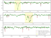 |
Fig. B.2. Example of a telluric-corrected spectrum with TelFit. The colour code is same as Fig. B.1. |
| In the text | |
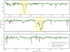 |
Fig. B.3. Example of a telluric-corrected spectrum with TAPAS. The colour code is same as Fig. B.1. |
| In the text | |
|
Fig. B.4. Example of a telluric-corrected spectrum with the standard star method. The colour code is same as Fig. B.1. |
| In the text | |
|
Fig. B.5. Example of a telluric-corrected spectrum with Molecfit. The colour code is same as Fig. B.1. |
| In the text | |
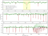 |
Fig. B.6. Example of a telluric-corrected spectrum with TelFit. The colour code is same as Fig. B.1. |
| In the text | |
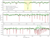 |
Fig. B.7. Example of a telluric-corrected spectrum with TAPAS. The colour code is same as Fig. B.1. |
| In the text | |
|
Fig. B.8. Example of a telluric-corrected spectrum with the standard star method. The colour code is same as Fig. B.1. |
| In the text | |
Current usage metrics show cumulative count of Article Views (full-text article views including HTML views, PDF and ePub downloads, according to the available data) and Abstracts Views on Vision4Press platform.
Data correspond to usage on the plateform after 2015. The current usage metrics is available 48-96 hours after online publication and is updated daily on week days.
Initial download of the metrics may take a while.