| Issue |
A&A
Volume 620, December 2018
|
|
|---|---|---|
| Article Number | A185 | |
| Number of page(s) | 25 | |
| Section | Catalogs and data | |
| DOI | https://doi.org/10.1051/0004-6361/201833621 | |
| Published online | 14 December 2018 | |
Long-term optical monitoring of TeV emitting blazars
I. Data analysis⋆
1
Finnish Centre for Astronomy with ESO (FINCA), University of Turku, Quantum, Vesilinnantie 5, 20014
Finland
e-mail: kani@utu.fi
2
Department of Physics and Astronomy, University of Turku, 20014
Finland
3
Agenzia Spaziale Italiana (ASI) Science Data Center, 00133
Roma, Italy
4
Istituto Nazionale di Fisica Nucleare, Sezione di Perugia, 06123
Perugia, Italy
5
Aalto University Metsähovi Radio Observatory, Metsähovintie 114, 02540
Kylmälä, Finland
6
Aalto University Department of Radio Science and Engineering, PO Box 13000
00076
Aalto, Finland
7
Dipartimento di Fisica, Università degli Studi di Torino, Via P. Giuria 1, 10125
Torino, Italy
8
Istituto Nazionale di Fisica Nucleare (INFN), Via P. Giuria 1, 10125
Torino, Italy
9
Department of Physics, University of Bath, Claverton Down, Bath, BA2 7AY
UK
Received:
12
June
2018
Accepted:
27
September
2018
We present ten years of R-band monitoring data of 31 northern blazars which were either detected at very high-energy (VHE) gamma rays or listed as potential VHE gamma-ray emitters. The data comprise 11 820 photometric data points in the R-band obtained in 2002–2012. We analyzed the light curves by determining their power spectral density (PSD) slopes assuming a power-law dependence with a single slope β and a Gaussian probability density function (PDF). We used the multiple fragments variance function (MFVF) combined with a forward-casting approach and likelihood analysis to determine the slopes and perform extensive simulations to estimate the uncertainties of the derived slopes. We also looked for periodic variations via Fourier analysis and quantified the false alarm probability through a large number of simulations. Comparing the obtained PSD slopes to values in the literature, we find the slopes in the radio band to be steeper than those in the optical and gamma rays. Our periodicity search yielded one target, Mrk 421, with a significant (p < 5%) period. Finding one significant period among 31 targets is consistent with the expected false alarm rate, but the period found in Mrk 421 is very strong and deserves further consideration.
Key words: galaxies: active / BL Lacertae objects: general / methods: data analysis
31 Photometric tables are only available at the CDS via anonymous ftp to cdsarc.u-strasbg.fr (130.79.128.5) or via http://cdsarc.u-strasbg.fr/viz-bin/qcat?J/A+A/620/A185
© ESO 2018
1. Introduction
Blazars are active galactic nuclei (AGN) with a relativistic jet that is pointing close to our line of sight. The blazar family consists of flat-spectrum radio quasars (FSRQs) and BL Lac objects. Blazars are the most numerous objects in the extragalactic gamma-ray sky. The spectral energy distribution of blazars shows two humps, one in the infrared to X-ray range and the second in the X-ray to gamma ray range. The first hump is ascribed to synchrotron emission and the second is typically attributed to inverse Compton (IC) emission. The peak frequency νpeak of the synchrotron peak is commonly used to further divide the BL Lacs into low-, intermediate-, and high-frequency peaked BL Lacs (LBL, IBL, and HBL, respectively) with logνpeak < 14 defining the LBL, 14 < logνpeak < 15 the IBL and logνpeak > 15 the HBL classes (Abdo et al. 2010a).
Blazars show variability in all bands from radio to very high-energy (VHE) gamma rays and on timescales ranging from years to only a few minutes. Sometimes there is correlated variability between two bands (e.g., Ramakrishnan et al. 2016, and references therein), but not always. The long-term variability has been most extensively studied in the radio and optical bands (e.g., Aller et al. 2003; Hovatta et al. 2007; Sillanpää et al. 1988; Villata et al. 2004), where long time series have been collected over decades. Blazar light curves are typically characterized by a power-law power spectral density (PSD), lacking clear and persistent periodicities and/or breaks in the spectrum, which would signify upper and lower limits for the variability timescales. The PSD is notoriously difficult to determine reliably due to uneven sampling and instrument noise (Scargle 1982; Hamuy & Maza 1989). In spite of these challenges, there have been several claims for periodicities in both radio and optical light curves of single sources (e.g., Sillanpää et al. 1988; Raiteri et al. 2001; Villata et al. 2004; Nesci 2010; King et al. 2013), but others have found no periodic changes in large sample of radio light curves (e.g., Hovatta et al. 2008). In recent years such searches have also become feasible in the gamma-ray band and, interestingly, common periodicities in optical and gamma rays have been reported for several sources (Sandrinelli et al. 2014; Ackermann et al. 2015; Sandrinelli et al. 2016a,b).
In this paper we present a detailed analysis of optical light curves of 31 blazars extending over 10 years. The data originate from the Tuorla Blazar monitoring program, which is introduced in Sect. 2, along with the sample selection. The observations and reduction processes are explained in Sect. 3, along with a detailed analysis of the variability, in particular the intrinsic power spectral density, and search for periodicities in the light curves is presented in Sect. 4. The entire flux data set is also published at the CDS for the first time.
2. Sample
The Tuorla Blazar Monitoring Program1 (Takalo et al. 2008) is an optical monitoring program that was started in September 2002. The monitoring program aims to support the VHE gamma-ray observations of the MAGIC Telescopes, and therefore the original sample consisted of 24 BL Lac objects from Costamante & Ghisellini (2002) with δ > +20°. These targets were predicted to emit VHE gamma rays and they are observable from the Tuorla Observatory over a large portion of the year. The sample has been gradually extended to include other types of gamma-ray emitting blazars and to the southern sky. Starting from 2004 most of the observations have been performed with the Kungliga Vetenskapsakademien (KVA) telescope on La Palma (see Sect. 3).
The sample discussed here consists of the original sample of 24 blazars from Costamante & Ghisellini (2002) along with seven additional well-sampled blazars. The targets are listed in Table 1 together with their most relevant properties. The sample covers all blazar classes, even though, due to the selection criteria, the HBLs are the most numerous sources in the sample. The large majority of the sources have been detected in VHE gamma-ray energies, some after triggers about high optical state from this monitoring program (e.g., 1ES1011+496, Mrk 180, ON325, S50716+714; Albert et al. 2007b, 2006b; Aleksić et al. 2012b; Anderhub et al. 2009a).
Main properties of the targets and observing log.
This paper presents photometric data for these 31 blazars from September 2002 to September 2012. Part of these data have been previously presented as light curves in papers reporting results of multiwavelength campaigns of individual blazars (see complete list in Table 1), looking for recurrent timescales and periodicities in the optical band (Ciprini et al. 2007; Takalo et al. 2010; Valtonen et al. 2016), common periodicities between the optical and gamma-ray bands (Ackermann et al. 2015), and in studies looking for correlations between different wavebands (e.g., Hayashida et al. 2012; Ackermann et al. 2014; Ramakrishnan et al. 2016; Jermak et al. 2016; Lindfors et al. 2016; Ahnen et al. 2016a). However, only a small portion of the data has been published in numerical form before (Villforth et al. 2010).
3. Observations and data reduction
The observations were made at two different telescopes using three different CCD cameras (see Table 2 for details). The Tuorla 1.03 m Dall-Kirkham telescope is located at Tuorla Observatory, Piikkiö, Finland, at 53 m above sea level. The focal length of the telescope is 8.45 m, which results in a field of view (FOV) of 10 × 10 arcmin with the ST-1001E chip. Typical seeing at the telescope is 3–6 arcsec and hence the CCD was binned by 2 × 2 pixels to obtain the pixel scale in Table 2. Depending on target brightness, three to eight exposures of 60 s each were obtained through the R-band filter. In addition to the science frames, five bias, dark, and dome flats were obtained. The CCD frames were reduced by first subtracting bias and dark and then dividing by the flat field.
Telescopes and CCD cameras used in the monitoring.
The KVA telescope is located at the Observatorio del Roque de los Muchachos (ORM) on La Palma, Spain, at 2396 m above sea level. The KVA system consists of two telescopes, a 60 cm telescope on a fork mount and a 35 cm Celestron-14 telescope bolted to the underbelly of the 60 cm telescope. All KVA data in this paper were obtained with the latter telescope, remotely operated from Finland. The 3.91 m focal length of the 35 cm telescope gave a FOV of 12 × 8 arcmin with the ST-8 chip and 11.6 × 11.6 arcmin with the U47 chip. Typical seeing during the observations was 1.5–3.5 arcsec, which required binning of the ST-8 chip by 2 × 2 pixels. Typical exposure times were 3 − 8 × 180 s, depending on object brightness. Calibration and image reduction was similar to the Tuorla data, except that the flat fields were obtained from twilight sky.
3.1. Photometry
Photometry of the targets was made in differential mode, i.e., by comparing the brightness of the object to the brightness of calibrated comparison stars near the target. Using multiple comparison stars improves the signal-to-noise ratio (S/N) of the photometry, but in a long-term project it is not guaranteed that all comparison stars are always within the FOV. Since the tabulated comparison star magnitudes always have errors, the derived zero point of the image depends on the stars chosen to calibrate the image. This effect is likely to be small since the above errors are usually small, a small fraction, but nevertheless we use only one comparison star that is sufficiently bright in order to obtain a good S/N. The observers were then instructed to always include this star within the FOV. Exceptions to this rule are Mkn 501 and 1ES 1959+650, for which only relatively weak calibrated comparison stars are available close to the target. For these targets two comparison stars were used. In addition to the comparison star, each field has a control star, whose photometry is performed identically to the target and which is used to identify possible problems during image reduction. Table 3 lists the comparison and control stars and their properties.
Comparison and control stars used in this work.
Photometry was performed with semiautomatic DIFFPHOT software developed at Tuorla Observatory. In short, DIFFPHOT reduces each image in turn as described above, displays the image on the screen, and waits for the user to point at the target. Then the software finds the comparison and control stars on the image using an internal database and computes accurate positions of the targets by computing the center of gravity of the light distribution. Aperture photometry is then performed at these positions. We used aperture radii rap between 4.0 and 7.5 arcsec depending on the object brightness (Table 3). To facilitate accurate host galaxy subtraction, the aperture was held constant for each target, except when the host galaxy contributed less than 3% to the total flux, in which case we used a smaller aperture for the KVA to take advantage of the better seeing. The chosen aperture sizes correspond roughly to the optimal aperture rap ≈ 1 − 1.5 FWHM (Howell 1989), except during the best seeing conditions at the KVA. However, this telescope sometimes was affected by bad tracking, resulting in elongated stars and the larger than optimal aperture size helped to compensate for this.
The sky background was determined from a circular annulus, sufficiently far from the target in order not to contaminate the sky region with target flux and devoid of any bright background/foreground targets. The sky pixel distribution was first sigma-cleaned and the mode of the distribution was computed from the formula

Using both sigma clipping and mode for sky estimation improve immunity against sky annulus contamination by background/foreground targets. The sky level was subtracted from the pixel values inside the aperture and the net counts N inside the aperture were computed, taking into account that some pixels are only partially inside the aperture. During this process and the aperture centering phase we also checked and eliminated highly deviant pixels inside the aperture by comparing the pixel value to the median of the six adjacent pixels. This check was inhibited within two pixels from the stellar core in order to not wrongly correct the central pixel when good seeing prevailed.
To calibrate the photometry we computed the scaling factor c from ADUs to Flux (Jy s ADU−1) for each image. The comparison star magnitude Rcomp was first transformed into flux Fcomp via
with F0 = 3080.0 Jy and then c was computed from
where Ncomp are the comparison star net counts in ADUs, ζ is the color term listed in Table 2 and Texp is the exposure time. The R-band fluxes of the target and the control star, F and Fctrl respectively, were then computed from
and
For the BL Lac nuclei we used V − R = 0.5, which corresponds to a power-law index α = 1.78 (Fν ∝ ν−α).
Finally, the data were averaged into one-hour bins to improve the S/N (formulae given below). These averaged fluxes Fa were then converted into R-band magnitudes via Eq. (2).
3.2. Error analysis
The averaged fluxes Fa derived above are affected by (i) statistical noise arising from photon, dark, and readout noise and image processing and (ii) systematic errors arising from assumptions of target and detector properties. The latter produce a systematic shift of the whole light curve, but do not change the flux differences between the data points and thus they are not included in the error bars. Below we discuss these errors in the order they appear in the error analysis.
Statistical variations in the fluxes in Eqs. (4) and (5) arise from the noise in observed counts N and the statistical noise in the scale factor c, the latter of which originates from the statistical noise in Ncomp via Eq. (3). The statistical errors of c, F, and Fctrl were determined by first computing the statistical errors of the corresponding observed counts Ncomp, N, and Nctrl from
where G is the gain factor (e−/ADU), σsky is the standard deviation of sky pixels, nap is the number of pixels in the aperture and nsky is the number of pixels in the sky annulus. We note that σsky is empirically measured from the image, so it includes the photon noise of the sky, dark noise, readout noise, and any residual noise from image processing. The statistical errors on target fluxes F are then obtained from
These errors were then used to compute the weighted average of the one hour bin Fa and its error σa from
and
Systematic flux errors arise in many ways from the color correction term 100.4 * ζ * (V − R) in Eqs. (4) and (5). First, since ζ varies from one instrument to another, small offsets between the three instruments are expected. We checked this by extracting the light curves of 31 control stars and measuring the systematic offsets between data obtained by different cameras. We found offsets between −0.051 and 0.050 mag, with 67% of the offsets between −0.011 and 0.019 mag. The target and control star data obtained by the KVA were shifted to the Tuorla data using these offsets, thereby suppressing the systematic differences between the cameras down to a level undetectable by our data. Second, our assumption of the same color V − R = 0.5 mag for all the targets is clearly too simple and in any case the color correction derived from stars is not an accurate model for blazars, which have different spectral energy distributions (SEDs) from the stars. Third, blazars display color variations, for example a “bluer when brighter” type of behavior (e.g., Ikejiri et al. 2011), which produces small brightness-dependent errors in our data. Given the zeta-values in Table 2 and the range of (V − R) color variations (∼0.1) mag, this error is negligible compared to the error bars.
We also checked whether the error bars σa obtained by the above procedure could be underestimated. We tested the control star light curves for variability using the chi-squared test with the null hypothesis that the stars are intrinsically nonvariable. The chi-squared statistic was computed from the formula
where ⟨F⟩ is the average flux of the light curve. We also computed the probability p that the null hypothesis can be rejected and assigned a limit p < 0.05 for a target to be considered variable.
Applying this procedure to the control stars, we found p < 0.01 for every control star. Rather than classifying all control stars variable, we assumed that the error bars derived from Eqs. (6)–(9) were too small. We thus added in quadrature an additional error term σs to the error bars σa and determined for each star the smallest σs which made the star nonvariable at the 5% level. Plotting the smallest σs against the average flux ⟨F⟩ (Fig. 1), we found that σs increases linearly with ⟨F⟩ with a slope of 0.0078 ± 0.0014 and an intercept of (9 ± 4) μJy. The linear dependence indicates that σs is always a constant fraction of the total flux, leading us to attribute this linear behavior to flat-fielding errors, which are multiplicative in nature. The intercept is barely significant, but we nevertheless included it in our noise model since such a noise limit is expected, and without this term the noise of faint targets is systematically underestimated. Since the relation above is an average dependence, adding σs from this relation makes ∼50% of the control stars nonvariable. To be consistent with the 5% variability limit, we thus multiplied this relation until only two of the control stars (6%) remained variable, resulting in
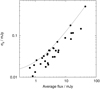 |
Fig. 1. Dependence of the additional error term σs on the average flux level. The solid line shows the relationship in Eq. (11), which makes 95% of the control stars nonvariable. This relationship is applied to our data. |

The final error bars σ for the binned average Fa is then obtained from
A small random error remains in the light curves of those blazars where the host galaxy component is relatively strong. Variable seeing causes different fractions of host galaxy and comparison star light to be included inside the aperture due to the difference in the surface brightness profiles (Carini et al. 1991; Cellone et al. 2000). However, for most of our targets this effect is very small. For instance, Mkn 501 has one of the strongest host galaxies in our sample and the effect of FWHM changing from 2 to 5 arcsec is ∼0.02 mag (see Fig. 3 in Nilsson et al. 2007). Targets with a nearby companion galaxy or a foreground star are most affected by the variable seeing. These targets are discussed in greater detail in Sect. 4.
In the tables at the CDS the errors have been converted into a magnitude errors σm via
i.e., the asymmetric magnitude errors have been made symmetric by taking the average of the upward and downward magnitude errors. The flux errors σ can be recovered from magnitude errors σm by marking
and using
To summarize our procedure: we first obtain the counts for the target, comparison star, and control star (N, Ncomp, and Nctrl, respectively) via aperture photometry. Then we determine c for each CCD frame from Eq. (3), the target and control star fluxes from Eqs. (4) and (5), and their errors from Eqs. (6) and (7). We compute one-hour averages using Eq. (8) and their errors from Eqs. (9)–(12). Finally we convert fluxes to magnitudes via Eqs. (2) and (13).
4. Analysis methods
As a first step in the analysis we subtracted the host galaxy contribution from the observed fluxes, corrected the light curves for the galactic extinction and applied the K-correction.
As was mentioned above, the presence of a host galaxy makes the fluxes to depend on both aperture and seeing. By using a constant aperture per target we have eliminated the aperture dependence, but an additional step was needed to account for the seeing effect. The host galaxy fluxes for different apertures and seeing conditions for the topmost 24 targets in Table 3 are tabulated in Nilsson et al. (2007). This work used observed, high-resolution (FWHM 0.5–1.0 arcsec) R-band images of our targets, convolved to a range of seeing values and measured with different aperture radii. We extracted from the tables in Nilsson et al. (2007) the host galaxy fluxes for each target using the corresponding measurement aperture and a seeing value of 2.0 arcsec for the KVA data and 5.0 arcsec for the Tuorla data. These values represent average seeing conditions at the two sites. Using different seeing values for the KVA and Tuorla data effectively reduces the shift between the two data sets, especially for 1ES 0120+340, Mkn 180, and 1ES 1544+820, all of which have a relatively strong nearby object leaking light into the measurement aperture. These targets are also most strongly affected by the varying seeing conditions, which increase their apparent variability.
For the seven targets not included in Nilsson et al. (2007) we used the analytical formulae in Graham & Driver (2005) and literature data to integrate the host galaxy light inside the aperture. These formulae do not take into account the smoothing by seeing, whose effect on the host galaxy fluxes is complicated due to the differential mode used. We thus applied the analytical formulae to the topmost 24 targets in Table 3 and checked the results against the more rigorously obtained values given in Nilsson et al. (2007). This comparison indicated that the analytic expression overestimates the host galaxy fluxes by only 3%. We thus divided the analytical host galaxy fluxes by 1.03 to be consistent with the other targets.
The galactic extinction was corrected by extracting the R-band extinction value AR from the NED2 and applying the correction. These values are based on the results in Schlegel et al. (1998). Finally, the light curves were corrected for the cosmological expansion by dividing the timescales by 1 + z and applying the K-correction by multiplying the fluxes by (1 + z)3 + α with α = 1.1 (Fν ∝ ν−α). The spectral slope chosen here corresponds to the mode of the α distribution of HBL in Fiorucci et al. (2004). The LBL generally have steeper spectra (αmode ∼ 1.5), so the transformed fluxes of LBL are likely to be underestimated. We note that performing this transform does not correct the light curves for the beaming effect caused by bulk relativistic motion in the jet.
4.1. Variability strength
As a general indicator of how variable our targets are, we use the chi-squared obtained by fitting a constant flux model to the data (Eq. (10)). This also provides us with the significance of the variations. Only significantly variable targets are submitted to further tests. As discussed above, the error bars include a noise-term scaled in such a way that the light curves of the control stars are consistent with a nonvariable target.
4.2. Synchrotron peak frequencies
In order to determine the peak frequency νpeak of the synchrotron component, we extracted the archival broadband flux data for all 31 targets from the Roma-BZCAT (5th Edition, Massaro et al. 2015) using the SED builder at the ASI Science Data Center3. In cases where there were few data points in the optical, we augmented the data with our host galaxy subtracted R-band monitoring data.
We simultaneously fit two log-parabolic spectra (e.g., Massaro et al. 2004), one for the synchrotron hump and another for the inverse Compton (IC) hump, to the broadband spectral energy distribution (SED) of the targets, including only data with logν/(Hz) > 8.5. Since the archival data are not simultaneous, and νpeak is known to change with the activity state in blazars (e.g., Anderhub et al. 2009b), we can expect the fitted νpeak to depend on the frequencies covered and on the number of observing epochs. To roughly estimate how much this could affect νpeak we binned the data starting from logν/(Hz)=8.5. The first bin had a width of 0.25 in log space, followed by bins increasing by a factor of two in width. We computed the mean flux in each bin and assigned an error bar equal to the standard error of the mean in each bin.
The two humps require eight parameters (Massaro et al. 2004); the two pivot energies were held constant and the remaining six were free. The fit was made by applying a Bayesian approach, sampling the posteriori distribution of the six free parameters with a Markov chain Monte Carlo (MCMC) sampler and with ensemble sampling and 30 walkers. At each iteration i, the synchrotron peak frequency  was computed from current parameters. Then the distribution of
  was used to determine νpeak and its uncertainty by a Gaussian fit made to this distribution.
The values of νpeak are listed in Table 5 and all the SEDs together with the best-fitting curve are shown in Fig. B.1. It is obvious that the radio part is poorly fitted, but this does not not seem to introduce a large shift in the fitted synchrotron component with respect to the data. However, it may add a small systematic error not taken into account by our error estimate. In some cases the IC peak fit can be considered questionable, but given that, for the most part of the synchrotron spectrum, the contribution of the IC peak is negligible, no large errors are expected for νpeak.
4.3. PSD power-law slope
Next we proceeded with estimating the slope of the intrinsic power spectral density (PSD) P(f) of the targets under the assumption that the PSD has a power-law form, i.e., P(f)∝fβ, where f is the temporal frequency in units of day−1 and β is the power-law slope. The PSD is equal to the square of the Fourier transform of the underlying time series. In practice we can only produce an estimate p(f) of P(f) by computing the discrete Fourier transform (DFT) of the observed time series. Inferring P(f) from p(f) is notoriously difficult due to the instrumental noise and the sampling effects (see, e.g., Uttley et al. 2002). The observed Fourier transform is a convolution of the true underlying Fourier transform and the window function W(x). The latter can be a very complicated function of f resulting in a distorted PSD p(f). Furthermore, due to the limited length of the times series and discrete sampling, the PSD can be estimated only within a limited window between fmin and fmax. If the true PSD contains significant power outside this window, limited data length and sampling cause power outside the window to leak into the window, further distorting the p(f). Especially in the case of a power-law PSD, power from frequencies below fmin, where the PSD is strongest, leaks into the frequency window (known as red noise leak).
Many different approaches have been developed over the years to overcome the problems associated with time series dominated by power-law noise (e.g., Emmanoulopoulos et al. 2010; Max-Moerbeck et al. 2014b; Vaughan et al. 2016). The most recent methods use an approach known as forward casting: starting from a model P(f), a large number of time series are generated with the same sampling and noise properties as in the observed data. The simulated sets are then used to derive an estimate of the statistical properties of P(f), and the observed data are tested against these distributions. By varying the model parameters, the best-fitting parameters can then be found by a suitable statistic. The distortions of P(f) are imprinted into the probability distributions and are thus naturally taken into account.
The sampling patterns of our light curves are highly irregular and contain large gaps due to the target being close to the Sun. Thus, we decided to reject any method relying on binning or interpolating in the time domain. We performed P(f) estimation using the multiple fractions variance function (MFVF) presented in Kastendieck et al. (2011).
The method (Kastendieck et al. 2011) studies the variance in the time series as a function of the time window. The algorithm works as follows. First, it computes the variance  of the whole time series and the corresponding frequency 1/Δt0, where Δt0 is the length of the data train. Next, it divides the times series into two fragments in the middle and computes the variances
  and
and  of the two subsets together with their corresponding frequencies. This process of subsequent halving is repeated until there are fewer than ten data points in a fragment. This process results in a set of variances σi over a number of frequencies fi = 1/Δti that can be analyzed with the same tools as the Fourier spectra.
Our procedure to estimate the PSD slope β is the following:
1. Let β vary from −2.8 to −1.0 with step 0.1. At each β repeat steps 2–8.
2. Generate 5000 evenly sampled light curves with a length of ∼100 times longer than the observed curve and a sampling of ten samples per day by inverse Fourier transform from the assumed model PSD:

(Fig. 2, upper left). The dense sampling ensures that the high frequencies of the power-law noise are properly presented in the data and that the long simulation length incorporates the red noise leak in the simulation. In our case the number of data points was 222 = 4 194 304. The time series are generated using the prescription of Timmer & Koenig (1995). We note that our model includes no flattening of the spectrum at low frequencies and the probability density function (PDF) of the time series is assumed to be Gaussian. Furthermore, our model does not implicitly include a white noise component. These points are discussed in more detail below.
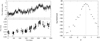 |
Fig. 2. Illustration of different phases of the analysis. Upper left panel: evenly sampled light curve generated with β = −1.4. This curve was cut from a longer set ∼100 times longer than shown here. Lower left panel: simulated curve resampled to the observing epochs of Mkn 421 and with instrumental noise added. Right panel: likelihood curve of Mkn 421 with the MFVF. The maximum of the polynomial fit (solid line) corresponds to β = −1.38. |
3. Resample the simulated light curves into the observing epochs (Fig. 2, lower left).
4. Scale the light curve to have the same variance as the observed data and add to each point a Gaussian random number with σ equal to the observational error of that point to simulate observational errors. The observed variance cannot be directly used to scale the simulated curve because the former contains instrumental noise, which increases the variance. We use the normalized excess variance (NXV; Nandra et al. 1997) to estimate the intrinsic variance  via the equation
![$$ \begin{aligned} \sigma _I^2 = \frac{1}{N} \sum _{k=1}^N \left[ (x(k) - \overline{x})^2 - \sigma _k^2 \right]\ , \end{aligned} $$](/articles/aa/full_html/2018/12/aa33621-18/aa33621-18-eq23.gif)
where  is the average of the data series and σk is the error of the kth data point. We then scale the simulated and resampled curve to have a variance equal to
  and add Gaussian random noise to each data point.
5. Compute the MFVF of the simulated curves.
6. Bin the MFVF data into frequency bins fi with roughly a factor of two increase in frequency per bin.
7. At each frequency bin fi, estimate the probability density function (PDF) p(fi) of the MFVF variance from the 5000 simulated values using Gaussian kernel density estimation.
8. Compute the log likelihood of β from
where p(fi) is the value of the PDF at fi and the summation is over all Nf frequency bins (Vaughan 2005, 2010). The MFVF transform uses variances in time windows of various lengths, so each point in the MFVF “spectrum” is distributed as chi-squared  , where n is the number of points in each time window. However, due to the possible effects of uneven sampling and the power-law nature of PSD, we do not use an analytical formula for p(fi). As explained in step 7, p(fi) was derived from the simulated spectra using a Gaussian kernel smoothing of the simulated points. The resulting values of p(fi) visually correspond to a chi-squared distribution with an appropriate degree of freedom, giving us further confidence that the simulations are producing correct results.
9. After scanning through the whole range in β, find the β corresponding to the maximum likelihood. The maximum was found by fitting a third-degree polynomial to the seven points straddling the highest likelihood found, and by finding the maximum of this polynomial. Figure 2 (right) shows a typical example of the likelihood curve and the fit.
Through Monte Carlo simulations, we tested the capability of the MFVF in recovering the correct power-law slope β. We generated 200 light curves with βin between −1.0 and −2.3 and ran the MFVF analysis on each of them. For the temporal sampling and instrumental noise we used the light curve of 3C 66A with 644 data points.
The results are summarized in Fig. 3. Two things are readily apparent from this figure: a) the capability to recover the correct power-law slope decreases when the input slope becomes steeper, and b) there is a small tendency to underestimate the slope, which is statistically significant in some cases, but nevertheless at least a factor of ∼2 smaller than the internal scatter.
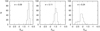 |
Fig. 3. Distributions of power-law slopes βout for three different input slopes βin, −1.0 (left panel), −1,5 (middle panel), and −2.3 (right panel) using the MFVF function. The rms scatter of the distributions are also indicated. |
We note that MFVF method is applied here in its simplest form, i.e., the results are computed directly from the observed points without binning or interpolating the data or applying any filtering technique. The performance of MFVF could probably be improved for steep power-law spectra with suitable filtering, but this is beyond the scope of this paper. In any case, all derived PSD slopes are > − 1.9, indicating that the most troublesome β range is mostly avoided in our study. We also note that although our PSD model Eq. (16) does not specify a white noise component, it is taken into account in step 4 where we add Gaussian noise to the simulated data points. When the simulated light curves are then transformed by the MFVM, this white noise gets imprinted into the probability density distribution at each frequency.
Errors on the derived β values were estimated by Monte Carlo simulations of artificial light curves, generated in the same way as in points 2–4 above. We generated 100 such curves, computed their PSDs and MFVF data, ran the likelihood analysis for each of the 100 curves, and recorded the rms scatter of the obtained β values.
4.4. Search for periodicities
The difficulty of reliably identifying a periodic signal in a red noise background has been discussed in detail by Vaughan (2005), among others. We estimated the PSD by computing the periodogram, i.e., the amplitude of the discrete Fourier transform of the light curve in the case of uneven sampling. Before computing the periodogram, the data were put into bins of 3.0 days in order to avoid dependencies between different frequencies. As in Vaughan (2005) we denote the true periodogram at frequencies fj = 1/Δtj with 𝒫(fj), the observed periodogram with I(fj), and the true probability density function (PDF) of 𝒫(fj) with p(fj).
We created 35 000 simulated light curves per target, again with similar mean, variance, and sampling as in the observed data and with the power-law slope derived in the previous step (Sect. 4.3). We then computed the periodogram I(fj) for each simulation and an estimate of the PDF p(fj), denoted here as  , from the ensemble of 35 000 points at each frequency fj via Gaussian kernel estimation. The large number of simulations was needed to sample the high end p(fj) > 0.99 properly. The probability that the power x at single frequency fj exceeds the observed value I(fj) was computed as
Since the possible periodic signal lies on top of a power-law background, it does not necessarily appear as the highest peak in the PSD. For this reason we chose the frequency with the highest significance (lowest P = Pmin) as a candidate for a periodic signal and computed the probability PN of finding such a peak in the absence of a periodic signal when N frequencies are examined from
Finally, we set PN < 5% as a limit for significant detection. In a sample of 31 targets we would then expect ∼2 targets to show significant periodicity by chance only.
5. Results
Here we list briefly the main results; we discuss them further in the next section. Table 4 gives a sample of the photometric tables, available for all 31 targets through Vizier4. A conversion from magnitudes to fluxes can be made through Eqs. (2), (14), and (15). We note that the presented magnitudes have not been corrected for galactic extinction or the host galaxy component.
Sample of the light curve data available at the CDS.
Main results of the analysis.
Figure A.1 shows on the left the light curves after subtracting the host galaxy and correcting for galactic extinction. The next panel shows the MVFV spectrum and the rightmost panel the periodogram. Figure B.1 shows the SEDs and their corresponding fits.
Table 5 summarizes the main results of our analysis. We show the reduced χ2 obtained by fitting a constant flux model to the target light curve (Col. 2), the synchrotron peak frequency νpeak from our fits (Col. 3). The BL Lac subclass division, Col. (4) (LBL/IBL/HBL in Table 1), is based on the value in Col. (3). The PSD slope β is shown (Col. 5) and the period with the highest significance (Col. 6) with its probability PN (Col. 7).
Using the chi-squared test, we find that the null hypothesis that the target flux does not vary with time can be rejected for all of our targets with p < 0.0001. As discussed above, the control stars are by design nonvariable by the same test. The 30 targets we analyzed therefore exhibit significant variability, so we apply our variability analysis to all of them, except to 1ES 1544+820, which has significantly lower number of data points compared to the other targets.
In Fig. 4 we plot the power-law slope β versus νpeak. A weak correlation seems to be present, so we tested the significance via a chi-squared test with the null hypothesis that the β values are drawn from a distribution β = β0. PKS 1510−089 was excluded from this analysis since its light is dominated by a single huge flare and our assumption of a power-law PSD with Gaussian PDF is clearly not valid. Fitting a constant β to the data we obtain βavg = −1.42, which we use as a surrogate for the population β0. Applying the chi-squared test yields  with a probability of p = 0.098 that the null hypothesis can be rejected, assuming our model of constant β is true. Thus, we do not find any significant deviation from a single PSD slope for our sample.
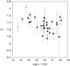 |
Fig. 4. Best-fitting PSD slope against synchrotron peak frequency. Filled symbols are BL Lacs, open symbols FSRQs. |
Our periodicity search finds a significant PSD peak in one target, Mkn 421 with a rest-frame period of 477 days. Finding one periodicity in 31 targets is consistent with the expected false alarm rate. Our result is thus consistent with no significant periodicities in any of our targets (but see discussion below on Mkn 421).
6. Discussion
6.1. PSD slopes
In Table 6 and Fig. 5 we compare our average PSD slope −1.42 ± 0.12 to the values in the literature obtained recently at radio, optical, and gamma rays for samples comparable in size to ours and by using similar methodology. Particularly, these studies considered carefully the distortions caused by uneven sampling and noise.
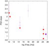 |
Fig. 5. PSD slope vs. observing frequency for samples of BL Lacs and a few individual targets. Filled red symbols: samples in Table 6; open purple square: FSRQ 3C 279 (this work); open purple circles: 3C 279 (Chatterjee et al. 2008); filled purple square: PKS 2155−304 (H.E.S.S. Collaboration 2017). |
PSD slopes of BL Lacs in recent studies.
The number of results is still small and it is not possible to draw firm conclusions, but a trend of decreasing beta with increasing frequency is apparent, or at the very least the radio slopes appear significantly different from the rest. The same trend seems to continue in the FSRQ 3C 279, although the results are more noisy for a single target compared to samples of targets. This result, if confirmed, would mean that in the regions emitting at radio frequencies variability preferentially occurs over long timescales, rather than over short timescales, i.e., the radio emitting regions have a longer “memory” of their previous state than the optical and gamma-ray emitting regions. This could simply be due to larger emitting volume in the radio than in the gamma rays and in the optical.
We emphasize, however, that although we fit a power-law PSD to the data, this does not imply that the underlying process is indeed a power-law process or even that the light curves at different wavebands result from the same process. For instance, the 22 and 37 GHz light curves of blazars can apparently be decomposed into a series of exponential flares (e.g., Valtaoja et al. 1999) with some regular features, like the decay timescale always being 1.3 times the rising timescale. A visual inspection of our optical light curves gives an impression that such a decomposition might be possible in some cases (e.g., 1ES 1959+650), but in most cases not. The apparent regularity in the radio suggests that the steeper PSD slope could simply be a result of fitting a noise process to a light curve that is not a result of such a process.
In the optical we do not find a significant correlation between the synchrotron peak frequency and the PSD slope, although it would not be unexpected. In low-peaked BL Lacs (LBL) the synchrotron peak is below the observation frequency and thus we are observing electrons in the high-energy tail of the energy distribution. In contrast, the optical emission from high-peaked BL Lacs (HBL) originates from electrons radiating below the peak energy. The cooling timescales of the high- and low-energy electrons are very different, and thus we might expect differences in the variability characteristics of LBL and HBL. However, our sample is not complete and contains only a few LBL. Therefore, such a correlation could be biased, if even found.
6.2. Periodicities
Looking at the sample as a whole, we did not find any evidence of periodic variations over the ten-year time span studied here. Our analysis takes into account the power-law background and is expected to be less sensitive to spurious peaks in the periodogram than many previous studies. We found significant periodicity (PN < 0.05) in one target only, a 477-day rest-frame period in Mkn 421. Finding one significant period among 31 targets is just what we would expect from chance alone.
However, the PSD peak in Mkn 421 is very strong, which warrants further consideration. Figure 6 shows the folded light curve of Mkn 421 over seven cycles. The variations seem consistently sinusoidal, except during the first ∼150 days of the cycle. There is thus an intriguing possibility of periodic variations in this source with extra activity triggered at certain phase of the cycle. Considering that we have tested the periodicity at > 100 frequencies over 31 targets, a chance coincidence cannot be completely ruled out, however. Li et al. (2016) found periods of 280–310 days in radio, X-ray and gamma-ray light curves of Mkn 421 in data spanning 6 to 10 years. The period found here is longer, but since we do not interpolate the spectrum in order to retain independence between the frequencies, our frequency resolution is quite low. Indeed, the adjacent frequencies in our PSD correspond to periods of 830 and 330 days. The difference cannot be completely explained by resolution only, but the actual difference cannot be well determined considering the differences in the analyses.
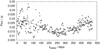 |
Fig. 6. Folded light curve of Mkn 421 using a rest-frame period of 477 days (gray symbols). The black line shows the harmonic function corresponding to the phase and amplitude in the periodogram. |
We finally comment on some periods claimed to have been found in our sample objects. Periodicities or quasiperiodicities have been claimed for S5 0716+714, but on much shorter timescales: e.g., 25–73 min (Gupta et al. 2009) or 15 min (Rani et al. 2010). Our sampling is too sparse to investigate this. In Pihajoki et al. (2013a) a 50-day period was found in OJ 287 from a two-year densely sampled data set taken in 2004–2006. This study used some of the same data as was used here, but there are very few common data points. Out of the 3991 data points in Pihajoki et al. (2013a), only about 140 originate from the data presented here. Our data also cover a time span longer than Pihajoki et al. (2013a) by a factor of ∼5 and hence the two data sets are largely independent. We find a very similar period of 52 days in the observed frame, but the significance is below our detection threshold. The folded light curve in Fig. 7 gives an indication of why the results could differ between different studies. There seems to be a stable periodic signal at low flux levels intermixed by a few high flux points at random phases. These high points are due to the double flares that occur in this source at ∼ 12-year intervals (e.g., Valtonen et al. 2006), which are very likely caused by a process completely unrelated to the periodic variations (Valtonen et al. 2016). The inclusion or exclusion of these flares will certainly affect the Fourier analysis, and pushes the result beyond the significance level in our case.
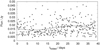 |
Fig. 7. Folded light curve of OJ 287 using a rest-frame period of 477 days (gray symbols). The black line shows the harmonic function corresponding to the phase and amplitude in the periodogram. |
Another significant periodicity reported recently is 798 ± 30 days found in the Fermi gamma-ray data for PG 1553+113, and further supported by optical data with a period of 754 ± 20 days (Ackermann et al. 2015). The significance of the optical PSD peak was reported to be < 5%. We do not detect this period in our data, although our data set is almost entirely included in Ackermann et al. (2015), forming about half of their sample. However, our frequency resolution is again very poor at periods of ∼800 days due to the relatively short time span with respect to this period. The fact that a similar timescale was found in gamma rays strengthens the case of significant periodic variations in PG 1553+113.
There are many other reports of detected periodicities, which we did not find here, like the optical 65-day period of 3C 66A (Lainela et al. 1999), or the ∼1-year optical periods tentatively but not conclusively detected in OJ 287, PKS 1510−089, and PKS 2155−304 by Sandrinelli et al. (2016a). Our analysis, and these examples, illustrate the difficulty of finding a weak periodic signal in a red noise background using data suffering from unknown systematic errors and sparse and uneven sampling (Vaughan et al. 2016). If persistent or recurrent periods were actually found, the timescale could shed some light onto their origin. The optical emission in BL Lacs is dominated by synchrotron emission from the jet, so periodic variations could be a result of a precession of the jet. This model has been used to explain, for example, the trajectories of the parsec-scale Very Long Baseline (VLBI) components in BL Lac (Caproni et al. 2013), although in this particular case no optical variations have been detected in the derived precession period of 12.1 years. Other possibilities exist, like a helical structure of the jet, which can form as a consequence of current-driven instabilities in the jet (Nakamura & Meier 2004).
Regular changes in the accretion mechanism that feeds the jet could also lead to periodic or quasiperiodic changes in the jet. Pihajoki et al. (2013a) attributed the 50-day period found in OJ 287 to a spiral density wave in the accretion disk and performed particle N-body simulations to show that a spiral wave configuration results in a periodic influx of material with approximately the same period as observed in OJ 287. Spiral density waves seem to be naturally generated around single (Li et al. 2001) and binary (Hanawa et al. 2010) black hole systems. In the former study, high-pressure vortices formed in the accretion disk, providing a natural source for increased accretion. In the latter study the spiral waves also exhibited oscillations, which could lead to episodes of periodic variations in the matter influx.
6.3. Caveats and future work
Our results and conclusions have to be taken with some caveats: first, we assume a Gaussian probability density function (PDF) when doing the simulations and second, our simulated spectra have no low- or high-frequency cutoffs. The assumption of Gaussian PDF is clearly not always valid and a log normal distribution would in many cases better represent the PDF, especially in targets whose light curve is dominated by a single or a few strong flares with apparently exponential growth and decay. Recently, a method has been presented to generate non-Gaussian light curves (Emmanoulopoulos et al. 2013), but the application of this procedure was left to future studies. Isobe et al. (2015) found their simulated x-ray PSDs of Mrk 421 to depend only slightly on the assumption of the PDF.
Since a power-law spectrum extending all the way to f = 0 would imply infinite power output, the PSDs of BL Lacs are expected to level off at some long timescale tb, which would reveal itself as a break in the spectrum at fb = 1/tb. Many of our PSDs show this kind of break, but these could be a result of finite data length rather than true breaks. Our simulations do not include this break as an input, but this is not necessarily a problem since the break timescale could be far longer than the ten-year interval studied here. In order to look for true breaks in blazar PSDs, long-term historical data needs to be collected and analyzed (as in e.g., Ciprini et al. 2007).
7. Conclusions
We have presented R-band monitoring data of 31 blazars (29 BL Lacs and 2 FSRQs) observed over a time span of ten years. In addition to presenting the light curves and describing in detail the data reduction process, we have analyzed the light curves by determining their PSD slopes and by searching for periodic variations in the light curves. These analyses were augmented by a substantial number of simulations to take into account the effects of uneven sampling and detector noise and to calibrate the false alarm rate of the periodicity search. Our results can be summarized as follows:
-
1)
We present for the first time all our R-band monitoring data in tabular form, altogether 11 820 photometric data points;
-
2)
By applying a chi-squared test we find that all 32 targets show significant variability with respect to the comparison stars;
-
3)
The average PSD slope of the 29 targets in our sample is −1.42 ± 0.12 (1σ standard deviation). The PSD slope is not significantly correlated (p = 9.8%) with the synchrotron peak frequency;
-
4)
Our average PSD slope
 is consistent with values found in the literature. Comparing our average PSD slope to those in the literature, we find that in the radio the slope tends to be steeper than in the optical and gamma-ray bands;
 -
5)
The periodicity search returned one target, Mkn 421, with a significant (p < 5%) peak in the periodogram. This is consistent with the expected false alarm rate, but the signal is Mrk 421 is very strong (p = 0.1%) and warrants further study with longer time span. We have not confirmed the 52-day period found in OJ 287 by us, but we note that high flare states caused by an unrelated emission process may complicate the analysis.
Acknowledgments
This paper is dedicated to the memory of our colleague and dear friend Leo Takalo 1952–2018, who played a crucial role in starting this monitoring effort and contributed significantly to the data acquisition. We would like to thank the Instituto de Astrofísica de Canarias for the excellent working conditions at the Observatorio del Roque de los Muchachos on La Palma. Part of this work is based on archival data, software, and online services provided by the ASI Space Science Data Center (ASI-SSDC). L.O. acknowledges partial support from the INFN Grant InDark and the grant of the Italian Ministry of Education, University and Research (MIUR) (L. 232/2016) “ECCELLENZA1822 D206 - Dipartimento di Eccellenza 2018-2022 Fisica” awarded to the Dept. of Physics of the University of Torino.
References
- Abdo, A. A., Ackermann, M., Agudo, I., et al. 2010a, ApJ, 716, 30 [NASA ADS] [CrossRef] [Google Scholar]
- Abdo, A. A., Ackermann, M., Ajello, M., et al. 2010b, Nature, 463, 919 [NASA ADS] [CrossRef] [PubMed] [Google Scholar]
- Abdo, A. A., Ackermann, M., Ajello, M., et al. 2011a, ApJ, 727, 129 [NASA ADS] [CrossRef] [Google Scholar]
- Abdo, A. A., Ackermann, M., Ajello, M., et al. 2011b, ApJ, 736, 131 [NASA ADS] [CrossRef] [Google Scholar]
- Acciari, V. A., Aliu, E., Aune, T., et al. 2009a, ApJ, 703, 169 [NASA ADS] [CrossRef] [Google Scholar]
- Acciari, V. A., Aliu, E., Aune, T., et al. 2009b, ApJ, 707, 612 [NASA ADS] [CrossRef] [Google Scholar]
- Acciari, V. A., Arlen, T., Aune, T., et al. 2011a, ApJ, 729, 2 [NASA ADS] [CrossRef] [Google Scholar]
- Acciari, V. A., Aliu, E., Arlen, T., et al. 2011b, ApJ, 738, 25 [NASA ADS] [CrossRef] [Google Scholar]
- Ackermann, M., Ajello, M., Allafort, A., et al. 2014, ApJ, 786, 157 [NASA ADS] [CrossRef] [Google Scholar]
- Ackermann, M., Ajello, M., Albert, A., et al. 2015, ApJ, 813, L41 [NASA ADS] [CrossRef] [Google Scholar]
- Ahnen, M. L., Ansoldi, S., Antonelli, L. A., et al. 2016a, A&A, 593, A91 [NASA ADS] [CrossRef] [EDP Sciences] [Google Scholar]
- Ahnen, M. L., Ansoldi, S., Antonelli, L. A., et al. 2016b, MNRAS, 459, 2286 [NASA ADS] [CrossRef] [Google Scholar]
- Albert, J., Aliu, E., Anderhub, H., et al. 2006a, ApJ, 639, 761 [NASA ADS] [CrossRef] [Google Scholar]
- Albert, J., Aliu, E., Anderhub, H., et al. 2006b, ApJ, 648, L105 [NASA ADS] [CrossRef] [Google Scholar]
- Albert, J., Aliu, E., Anderhub, H., et al. 2007a, ApJ, 654, L119 [NASA ADS] [CrossRef] [Google Scholar]
- Albert, J., Aliu, E., Anderhub, H., et al. 2007b, ApJ, 667, L21 [NASA ADS] [CrossRef] [Google Scholar]
- Albert, J., Aliu, E., Anderhub, H., et al. 2007c, ApJ, 662, 892 [NASA ADS] [CrossRef] [Google Scholar]
- Albert, J., Aliu, E., Anderhub, H., et al. 2007d, ApJ, 666, L17 [NASA ADS] [CrossRef] [Google Scholar]
- Albert, J., Aliu, E., Anderhub, H., et al. 2007e, ApJ, 669, 862 [NASA ADS] [CrossRef] [Google Scholar]
- Albert, J., Aliu, E., Anderhub, H., et al. 2009, A&A, 493, 467 [NASA ADS] [CrossRef] [EDP Sciences] [Google Scholar]
- Aleksić, J., Anderhub, H., Antonelli, L. A., et al. 2010a, A&A, 515, A76 [NASA ADS] [CrossRef] [EDP Sciences] [Google Scholar]
- Aleksić, J., Anderhub, H., Antonelli, L. A., et al. 2010b, A&A, 519, A32 [NASA ADS] [CrossRef] [EDP Sciences] [Google Scholar]
- Aleksić, J., Antonelli, L. A., Antoranz, P., et al. 2010c, A&A, 524, A77 [NASA ADS] [CrossRef] [EDP Sciences] [Google Scholar]
- Aleksić, J., Antonelli, L. A., Antoranz, P., et al. 2011, A&A, 530, A4 [NASA ADS] [CrossRef] [EDP Sciences] [Google Scholar]
- Aleksić, J., Alvarez, E. A., Antonelli, L. A., et al. 2012a, A&A, 542, A100 [NASA ADS] [CrossRef] [EDP Sciences] [Google Scholar]
- Aleksić, J., Alvarez, E. A., Antonelli, L. A., et al. 2012b, A&A, 544, A142 [NASA ADS] [CrossRef] [EDP Sciences] [Google Scholar]
- Aleksić, J., Alvarez, E. A., Antonelli, L. A., et al. 2012c, ApJ, 748, 46 [NASA ADS] [CrossRef] [Google Scholar]
- Aleksić, J., Antonelli, L. A., Antoranz, P., et al. 2013, A&A, 556, A67 [NASA ADS] [CrossRef] [EDP Sciences] [Google Scholar]
- Aleksić, J., Antonelli, L. A., Antoranz, P., et al. 2014a, A&A, 563, A90 [NASA ADS] [CrossRef] [EDP Sciences] [Google Scholar]
- Aleksić, J., Ansoldi, S., Antonelli, L. A., et al. 2014b, A&A, 567, A41 [NASA ADS] [CrossRef] [EDP Sciences] [Google Scholar]
- Aleksić, J., Ansoldi, S., Antonelli, L. A., et al. 2014c, A&A, 567, A135 [NASA ADS] [CrossRef] [EDP Sciences] [Google Scholar]
- Aleksić, J., Ansoldi, S., Antonelli, L. A., et al. 2014d, A&A, 569, A46 [NASA ADS] [CrossRef] [EDP Sciences] [Google Scholar]
- Aleksić, J., Ansoldi, S., Antonelli, L. A., et al. 2015a, MNRAS, 446, 217 [NASA ADS] [CrossRef] [Google Scholar]
- Aleksić, J., Ansoldi, S., Antonelli, L. A., et al. 2015b, A&A, 573, A50 [NASA ADS] [CrossRef] [EDP Sciences] [Google Scholar]
- Aleksić, J., Ansoldi, S., Antonelli, L. A., et al. 2015c, A&A, 576, A126 [NASA ADS] [CrossRef] [EDP Sciences] [Google Scholar]
- Aleksić, J., Ansoldi, S., Antonelli, L. A., et al. 2015d, A&A, 578, A22 [NASA ADS] [CrossRef] [EDP Sciences] [Google Scholar]
- Aleksić, J., Ansoldi, S., Antonelli, L. A., et al. 2015e, MNRAS, 450, 4399 [NASA ADS] [CrossRef] [Google Scholar]
- Aleksić, J., Ansoldi, S., Antonelli, L. A., et al. 2015f, MNRAS, 451, 739 [NASA ADS] [CrossRef] [Google Scholar]
- Aleksić, J., Ansoldi, S., Antonelli, L. A., et al. 2016, A&A, 591, A10 [NASA ADS] [CrossRef] [EDP Sciences] [Google Scholar]
- Aliu, E., Anderhub, H., Antonelli, L. A., et al. 2009, ApJ, 692, L29 [NASA ADS] [CrossRef] [Google Scholar]
- Aller, M. F., Aller, H. D., & Hughes, P. A. 2003, ApJ, 586, 33 [NASA ADS] [CrossRef] [Google Scholar]
- Anderhub, H., Antonelli, L. A., Antoranz, P., et al. 2009a, ApJ, 704, L129 [NASA ADS] [CrossRef] [Google Scholar]
- Anderhub, H., Antonelli, L. A., Antoranz, P., et al. 2009b, ApJ, 705, 1624 [NASA ADS] [CrossRef] [Google Scholar]
- Bhatta, G., Webb, J. R., Hollingsworth, H., et al. 2013, A&A, 558, A92 [NASA ADS] [CrossRef] [EDP Sciences] [Google Scholar]
- Böttcher, M., Basu, S., Joshi, M., et al. 2007, ApJ, 670, 968 [NASA ADS] [CrossRef] [Google Scholar]
- Böttcher, M., Fultz, K., Aller, H. D., et al. 2009, ApJ, 694, 174 [NASA ADS] [CrossRef] [Google Scholar]
- Caproni, A., Abraham, Z., & Monteiro, H. 2013, MNRAS, 428, 280 [NASA ADS] [CrossRef] [Google Scholar]
- Carini, M. T., Miller, H. R., Noble, J. C., & Sadun, A. C. 1991, AJ, 101, 1196 [NASA ADS] [CrossRef] [Google Scholar]
- Cellone, S. A., Romero, G. E., & Combi, J. A. 2000, AJ, 119, 1534 [NASA ADS] [CrossRef] [Google Scholar]
- Chatterjee, R., Jorstad, S. G., Marscher, A. P., et al. 2008, ApJ, 689, 79 [NASA ADS] [CrossRef] [Google Scholar]
- Ciprini, S., Takalo, L. O., Tosti, G., et al. 2007, A&A, 467, 465 [NASA ADS] [CrossRef] [EDP Sciences] [Google Scholar]
- Costamante, L., & Ghisellini, G. 2002, A&A, 384, 56 [NASA ADS] [CrossRef] [EDP Sciences] [Google Scholar]
- D’Ammando, F., Pucella, G., Raiteri, C. M., et al. 2009, A&A, 508, 181 [NASA ADS] [CrossRef] [EDP Sciences] [Google Scholar]
- D’Ammando, F., Raiteri, C. M., Villata, M., et al. 2011, A&A, 529, A145 [NASA ADS] [CrossRef] [EDP Sciences] [Google Scholar]
- Donnarumma, I., Vittorini, V., Vercellone, S., et al. 2009, ApJ, 691, L13 [NASA ADS] [CrossRef] [Google Scholar]
- Emmanoulopoulos, D., McHardy, I. M., & Uttley, P. 2010, MNRAS, 404, 931 [NASA ADS] [CrossRef] [Google Scholar]
- Emmanoulopoulos, D., McHardy, I. M., & Papadakis, I. E. 2013, MNRAS, 433, 907 [NASA ADS] [CrossRef] [Google Scholar]
- Fiorucci, M., & Tosti, G. 1996, A&AS, 116, 403 [NASA ADS] [CrossRef] [EDP Sciences] [Google Scholar]
- Fiorucci, M., Tosti, G., & Rizzi, N. 1998, PASP, 110, 105 [NASA ADS] [CrossRef] [Google Scholar]
- Fiorucci, M., Ciprini, S., & Tosti, G. 2004, A&A, 419, 25 [NASA ADS] [CrossRef] [EDP Sciences] [Google Scholar]
- Graham, A. W., & Driver, S. P. 2005, PASA, 22, 118 [NASA ADS] [CrossRef] [Google Scholar]
- Gupta, A. C., Srivastava, A. K., & Wiita, P. J. 2009, ApJ, 690, 216 [NASA ADS] [CrossRef] [Google Scholar]
- Hamuy, M., & Maza, J. 1989, AJ, 97, 720 [NASA ADS] [CrossRef] [Google Scholar]
- Hanawa, T., Ochi, Y., & Ando, K. 2010, ApJ, 708, 485 [NASA ADS] [CrossRef] [Google Scholar]
- Hayashida, M., Madejski, G. M., Nalewajko, K., et al. 2012, ApJ, 754, 114 [NASA ADS] [CrossRef] [Google Scholar]
- H.E.S.S. Collaboration (Abdalla, H., et al.) 2017, A&A, 598, A39 [NASA ADS] [CrossRef] [EDP Sciences] [Google Scholar]
- Hovatta, T., Tornikoski, M., Lainela, M., et al. 2007, A&A, 469, 899 [NASA ADS] [CrossRef] [EDP Sciences] [Google Scholar]
- Hovatta, T., Lehto, H. J., & Tornikoski, M. 2008, A&A, 488, 897 [NASA ADS] [CrossRef] [EDP Sciences] [Google Scholar]
- Howell, S. B. 1989, PASP, 101, 616 [NASA ADS] [CrossRef] [Google Scholar]
- Ikejiri, Y., Uemura, M., Sasada, M., et al. 2011, PASJ, 63, 639 [NASA ADS] [Google Scholar]
- Isobe, N., Sato, R., Ueda, Y., et al. 2015, ApJ, 798, 27 [NASA ADS] [CrossRef] [Google Scholar]
- Jermak, H., Steele, I. A., Lindfors, E., et al. 2016, MNRAS, 462, 4267 [NASA ADS] [CrossRef] [Google Scholar]
- Kastendieck, M. A., Ashley, M. C. B., & Horns, D. 2011, A&A, 531, A123 [NASA ADS] [CrossRef] [EDP Sciences] [Google Scholar]
- Kiehlmann, S., Savolainen, T., Jorstad, S. G., et al. 2016, A&A, 590, A10 [NASA ADS] [CrossRef] [EDP Sciences] [Google Scholar]
- King, O. G., Hovatta, T., Max-Moerbeck, W., et al. 2013, MNRAS, 436, L114 [NASA ADS] [CrossRef] [Google Scholar]
- Lainela, M., Takalo, L. O., Sillanpää, A., et al. 1999, ApJ, 521, 561 [NASA ADS] [CrossRef] [Google Scholar]
- Larionov, V. M., Jorstad, S. G., Marscher, A. P., et al. 2008, A&A, 492, 389 [NASA ADS] [CrossRef] [EDP Sciences] [Google Scholar]
- Li, H., Colgate, S. A., Wendroff, B., & Liska, R. 2001, ApJ, 551, 874 [NASA ADS] [CrossRef] [Google Scholar]
- Li, H. Z., Jiang, Y. G., Guo, D. F., Chen, X., & Yi, T. F. 2016, PASP, 128, 074101 [NASA ADS] [CrossRef] [Google Scholar]
- Lichti, G. G., Bottacini, E., Ajello, M., et al. 2008, A&A, 486, 721 [NASA ADS] [CrossRef] [EDP Sciences] [Google Scholar]
- Lindfors, E. J., Hovatta, T., Nilsson, K., et al. 2016, A&A, 593, A98 [NASA ADS] [CrossRef] [EDP Sciences] [Google Scholar]
- MAGIC Collaboration, Albert, J., Aliu, E., et al. 2008, Science, 320, 1752 [NASA ADS] [CrossRef] [PubMed] [Google Scholar]
- Massaro, E., Perri, M., Giommi, P., & Nesci, R. 2004, A&A, 413, 489 [NASA ADS] [CrossRef] [EDP Sciences] [Google Scholar]
- Massaro, E., Maselli, A., Leto, C., et al. 2015, ApSS, 357, 75 [Google Scholar]
- Max-Moerbeck, W., Hovatta, T., Richards, J. L., et al. 2014a, MNRAS, 445, 428 [NASA ADS] [CrossRef] [Google Scholar]
- Max-Moerbeck, W., Richards, J. L., Hovatta, T., et al. 2014b, MNRAS, 445, 437 [NASA ADS] [CrossRef] [Google Scholar]
- Nakamura, M., & Meier, D. L. 2004, ApJ, 617, 123 [NASA ADS] [CrossRef] [Google Scholar]
- Nandra, K., George, I. M., Mushotzky, R. F., Turner, T. J., & Yaqoob, T. 1997, ApJ, 476, 70 [NASA ADS] [CrossRef] [Google Scholar]
- Nesci, R. 2010, AJ, 139, 2425 [NASA ADS] [CrossRef] [Google Scholar]
- Nilsson, K., Pasanen, M., Takalo, L. O., et al. 2007, A&A, 475, 199 [NASA ADS] [CrossRef] [EDP Sciences] [Google Scholar]
- Ostorero, L., Wagner, S. J., Gracia, J., et al. 2006, A&A, 451, 797 [NASA ADS] [CrossRef] [EDP Sciences] [Google Scholar]
- Pian, E., Foschini, L., Beckmann, V., et al. 2005, A&A, 429, 427 [NASA ADS] [CrossRef] [EDP Sciences] [Google Scholar]
- Pihajoki, P., Valtonen, M., & Ciprini, S. 2013a, MNRAS, 434, 3122 [NASA ADS] [CrossRef] [Google Scholar]
- Pihajoki, P., Valtonen, M., Zola, S., et al. 2013b, ApJ, 764, 5 [NASA ADS] [CrossRef] [Google Scholar]
- Raiteri, C. M., Villata, M., Lanteri, L., Cavallone, M., & Sobrito, G. 1998, A&AS, 130, 495 [NASA ADS] [CrossRef] [EDP Sciences] [Google Scholar]
- Raiteri, C. M., Villata, M., Aller, H. D., et al. 2001, A&A, 377, 396 [NASA ADS] [CrossRef] [EDP Sciences] [Google Scholar]
- Raiteri, C. M., Villata, M., D’Ammando, F., et al. 2013, MNRAS, 436, 1530 [NASA ADS] [CrossRef] [Google Scholar]
- Ramakrishnan, V., Hovatta, T., Nieppola, E., et al. 2015, MNRAS, 452, 1280 [CrossRef] [Google Scholar]
- Ramakrishnan, V., Hovatta, T., Tornikoski, M., et al. 2016, MNRAS, 456, 171 [NASA ADS] [CrossRef] [Google Scholar]
- Rani, B., Gupta, A. C., Joshi, U. C., Ganesh, S., & Wiita, P. J. 2010, ApJ, 719, L153 [NASA ADS] [CrossRef] [Google Scholar]
- Sandrinelli, A., Covino, S., & Treves, A. 2014, ApJ, 793, L1 [NASA ADS] [CrossRef] [Google Scholar]
- Sandrinelli, A., Covino, S., Dotti, M., & Treves, A. 2016a, AJ, 151, 54 [NASA ADS] [CrossRef] [Google Scholar]
- Sandrinelli, A., Covino, S., & Treves, A. 2016b, ApJ, 820, 20 [NASA ADS] [CrossRef] [Google Scholar]
- Scargle, J. D. 1982, ApJ, 263, 835 [NASA ADS] [CrossRef] [Google Scholar]
- Schlegel, D. J., Finkbeiner, D. P., & Davis, M. 1998, ApJ, 500, 525 [NASA ADS] [CrossRef] [Google Scholar]
- Sillanpää, A., Haarala, S., Valtonen, M. J., Sundelius, B., & Byrd, G. G. 1988, ApJ, 325, 628 [NASA ADS] [CrossRef] [Google Scholar]
- Smith, P. S., Jannuzi, B. T., & Elston, R. 1991, ApJS, 77, 67 [NASA ADS] [CrossRef] [Google Scholar]
- Sobolewska, M. A., Siemiginowska, A., Kelly, B. C., & Nalewajko, K. 2014, ApJ, 786, 143 [NASA ADS] [CrossRef] [Google Scholar]
- Tagliaferri, G., Foschini, L., Ghisellini, G., et al. 2008, ApJ, 679, 1029 [NASA ADS] [CrossRef] [Google Scholar]
- Takalo, L. O., Nilsson, K., Lindfors, E., et al. 2008, in AIP Conf. Ser., eds. F. A. Aharonian, W. Hofmann, F. Rieger, 1085, 705 [NASA ADS] [CrossRef] [Google Scholar]
- Takalo, L. O., Hagen-Thorn, V. A., Hagen-Thorn, E. I., Ciprini, S., & Sillanpää, A. 2010, A&A, 517, A63 [NASA ADS] [CrossRef] [EDP Sciences] [Google Scholar]
- Timmer, J., & Koenig, M. 1995, A&A, 300, 707 [NASA ADS] [Google Scholar]
- Uttley, P., McHardy, I. M., & Papadakis, I. E. 2002, MNRAS, 332, 231 [NASA ADS] [CrossRef] [Google Scholar]
- Valtaoja, E., Lähteenmäki, A., Teräsranta, H., & Lainela, M. 1999, ApJS, 120, 95 [NASA ADS] [CrossRef] [Google Scholar]
- Valtonen, M. J., Lehto, H. J., Sillanpää, A., et al. 2006, ApJ, 646, 36 [NASA ADS] [CrossRef] [Google Scholar]
- Valtonen, M. J., Lehto, H. J., Nilsson, K., et al. 2008, Nature, 452, 851 [NASA ADS] [CrossRef] [PubMed] [Google Scholar]
- Valtonen, M. J., Nilsson, K., Villforth, C., et al. 2009, ApJ, 698, 781 [NASA ADS] [CrossRef] [Google Scholar]
- Valtonen, M. J., Zola, S., Ciprini, S., et al. 2016, ApJ, 819, L37 [NASA ADS] [CrossRef] [Google Scholar]
- Vaughan, S. 2005, A&A, 431, 391 [NASA ADS] [CrossRef] [EDP Sciences] [Google Scholar]
- Vaughan, S. 2010, MNRAS, 402, 307 [NASA ADS] [CrossRef] [Google Scholar]
- Vaughan, S., Uttley, P., Markowitz, A. G., et al. 2016, MNRAS, 461, 3145 [NASA ADS] [CrossRef] [Google Scholar]
- Villata, M., Raiteri, C. M., Ghisellini, G., et al. 1997, A&AS, 121, 119 [NASA ADS] [CrossRef] [EDP Sciences] [Google Scholar]
- Villata, M., Raiteri, C. M., Lanteri, L., Sobrito, G., & Cavallone, M. 1998, A&AS, 130, 305 [NASA ADS] [CrossRef] [EDP Sciences] [MathSciNet] [PubMed] [Google Scholar]
- Villata, M., Raiteri, C. M., Aller, H. D., et al. 2004, A&A, 424, 497 [NASA ADS] [CrossRef] [EDP Sciences] [Google Scholar]
- Villata, M., Raiteri, C. M., Larionov, V. M., et al. 2008, A&A, 481, L79 [NASA ADS] [CrossRef] [EDP Sciences] [Google Scholar]
- Villata, M., Raiteri, C. M., Larionov, V. M., et al. 2009, A&A, 501, 455 [NASA ADS] [CrossRef] [EDP Sciences] [Google Scholar]
- Villforth, C., Nilsson, K., Heidt, J., et al. 2010, MNRAS, 402, 2087 [NASA ADS] [CrossRef] [Google Scholar]
Appendix A: Light curves
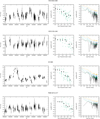 |
Fig. A.1. Left panels: observed light curve. Middle panels: multiple fragments variance function (MFVF). Gray dots show the unbinned values and black dots the binned values. Right panels: power spectral density (PSD) together with 67%, 95%, and 99.9% limits for a single frequency, taking into account the number of frequencies covered. The two rightmost panels were computed from data transformed to the rest frame. |
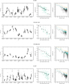 |
Fig. A.1. continued. |
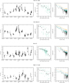 |
Fig. A.1. continued. |
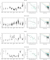 |
Fig. A.1. continued. |
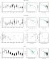 |
Fig. A.1. continued. |
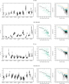 |
Fig. A.1. continued. |
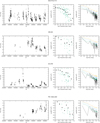 |
Fig. A.1. continued. |
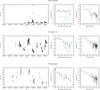 |
Fig. A.1. continued. |
Appendix B: Spectral energy distributions
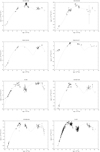 |
Fig. B.1. Archive spectral energy distribution data used to determine the synchrotron peak frequency. The dotted line shows the best-fit model. |
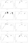 |
Fig. B.1. continued. |
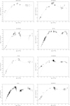 |
Fig. B.1. continued. |
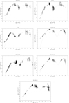 |
Fig. B.1. continued. |
All Tables
All Figures
|
Fig. 1. Dependence of the additional error term σs on the average flux level. The solid line shows the relationship in Eq. (11), which makes 95% of the control stars nonvariable. This relationship is applied to our data. |
| In the text | |
|
Fig. 2. Illustration of different phases of the analysis. Upper left panel: evenly sampled light curve generated with β = −1.4. This curve was cut from a longer set ∼100 times longer than shown here. Lower left panel: simulated curve resampled to the observing epochs of Mkn 421 and with instrumental noise added. Right panel: likelihood curve of Mkn 421 with the MFVF. The maximum of the polynomial fit (solid line) corresponds to β = −1.38. |
| In the text | |
|
Fig. 3. Distributions of power-law slopes βout for three different input slopes βin, −1.0 (left panel), −1,5 (middle panel), and −2.3 (right panel) using the MFVF function. The rms scatter of the distributions are also indicated. |
| In the text | |
|
Fig. 4. Best-fitting PSD slope against synchrotron peak frequency. Filled symbols are BL Lacs, open symbols FSRQs. |
| In the text | |
|
Fig. 5. PSD slope vs. observing frequency for samples of BL Lacs and a few individual targets. Filled red symbols: samples in Table 6; open purple square: FSRQ 3C 279 (this work); open purple circles: 3C 279 (Chatterjee et al. 2008); filled purple square: PKS 2155−304 (H.E.S.S. Collaboration 2017). |
| In the text | |
|
Fig. 6. Folded light curve of Mkn 421 using a rest-frame period of 477 days (gray symbols). The black line shows the harmonic function corresponding to the phase and amplitude in the periodogram. |
| In the text | |
|
Fig. 7. Folded light curve of OJ 287 using a rest-frame period of 477 days (gray symbols). The black line shows the harmonic function corresponding to the phase and amplitude in the periodogram. |
| In the text | |
|
Fig. A.1. Left panels: observed light curve. Middle panels: multiple fragments variance function (MFVF). Gray dots show the unbinned values and black dots the binned values. Right panels: power spectral density (PSD) together with 67%, 95%, and 99.9% limits for a single frequency, taking into account the number of frequencies covered. The two rightmost panels were computed from data transformed to the rest frame. |
| In the text | |
|
Fig. A.1. continued. |
| In the text | |
|
Fig. A.1. continued. |
| In the text | |
|
Fig. A.1. continued. |
| In the text | |
|
Fig. A.1. continued. |
| In the text | |
|
Fig. A.1. continued. |
| In the text | |
|
Fig. A.1. continued. |
| In the text | |
|
Fig. A.1. continued. |
| In the text | |
|
Fig. B.1. Archive spectral energy distribution data used to determine the synchrotron peak frequency. The dotted line shows the best-fit model. |
| In the text | |
|
Fig. B.1. continued. |
| In the text | |
|
Fig. B.1. continued. |
| In the text | |
|
Fig. B.1. continued. |
| In the text | |
Current usage metrics show cumulative count of Article Views (full-text article views including HTML views, PDF and ePub downloads, according to the available data) and Abstracts Views on Vision4Press platform.
Data correspond to usage on the plateform after 2015. The current usage metrics is available 48-96 hours after online publication and is updated daily on week days.
Initial download of the metrics may take a while.