| Issue |
A&A
Volume 619, November 2018
|
|
|---|---|---|
| Article Number | A84 | |
| Number of page(s) | 8 | |
| Section | Stellar structure and evolution | |
| DOI | https://doi.org/10.1051/0004-6361/201833693 | |
| Published online | 08 November 2018 | |
When nature tries to trick us
An eclipsing eccentric close binary superposed on the central star of the planetary nebula M 3-2⋆,⋆⋆
1
European Southern Observatory, Karl-Schwarzschild-str. 2, 85748 Garching, Germany
e-mail: This email address is being protected from spambots. You need JavaScript enabled to view it.
2
Instituto de Astrofísica de Canarias, Vía Láctea s/n, 38200 La Laguna, Tenerife, Spain
3
Departamento de Astrofísica, Universidad de La Laguna, 38206 La Laguna, Tenerife, Spain
4
Department of Physics and Astronomy, University College London, Gower St, London, WC1E 6BT, UK
5
Las Campanas Observatory, Carnegie Institution of Washington, La Serena, Chile
6
South African Astronomical Observatory, PO Box 9, Observatory 7935, South Africa
7
Southern African Large Telescope Foundation, PO Box 9, Observatory 7935, South Africa
8
European Southern Observatory, Alonso de Córdova 3107, Casilla, 19001, Santiago Chile
9
Departamento de Ciencias Físicas, Universidad Andres Bello, Fernández Concha 700, Las Condes, Santiago
10
GRANTECAN, Cuesta de San José s/n, 38712 Breña Baja, La Palma, Spain
11
Observatorio Astronómico Nacional (OAN-IGN), C/Alfonso XII 3, 28014 Madrid, Spain
Received:
21
June
2018
Accepted:
27
July
2018
Abstract
Bipolar planetary nebulae (PNe) are thought to result from binary star interactions and, indeed, tens of binary central stars of PNe have been found, in particular using photometric time-series that allow for the detection of post-common envelope systems. Using photometry at the NTT in La Silla we have studied the bright object close to the centre of PN M 3-2 and found it to be an eclipsing binary with an orbital period of 1.88 days. However, the components of the binary appear to be two A or F stars, of almost equal mass, and are therefore too cold to be the source of ionisation of the nebula. Using deep images of the central star obtained in good seeing conditions, we confirm a previous result that the central star is more likely much fainter, located 2″ away from the bright star. The eclipsing binary is thus a chance alignment on top of the planetary nebula. We also studied the nebular abundance and confirm it to be a Type I PN.
Key words: methods: observational / binaries: eclipsing / stars: early-type / planetary nebulae: individual: PN G240.3-07.6 / stars: AGB and post-AGB
Based on ESO observations made under programmes 088.D-0573(A), 090.D-0435(A), 090.D-0693(A), 091.D-0475(A), 092.D-0449(A), 094.D-0031(A), 094.D-0031(A), and 096.D-0237(A).
Tables A.1 and A.2 are only available at the CDS via anonymous ftp to cdsarc.u-strasbg.fr (130.79.125.5) or via http://cdsweb.u-strasbg.fr/cgi-bin/qcat?J/A+A/619/A84
© ESO 2018
1. The bipolar nebula M 3-2
Planetary nebulae (PNe) are thought to be short episodes at the end of the lives of intermediate-mass stars, just before they become white dwarfs. Most planetary nebulae come, however, in many different shapes, which is difficult to explain in the case of the evolution of a single star (Balick & Frank 2002). This is particularly true for bipolar planetary nebulae, for which there is now mounting evidence that they originate from a binary system (Miszalski et al. 2009, 2018; De Marco 2009; Boffin 2015a,b; Jones & Boffin 2017a). Furthermore, many close binaries are now found at the centre of planetary nebulae1.
PN M 3-2 (PN G240.3-07.6, ESO 428-5; Minkowski 1948) is a bipolar type I planetary nebula with a well defined ring (Fig. A.1), making it a perfect contender to host a binary system according to the observed correlation between nebular morphology and central star binarity (Miszalski et al. 2009; Jones et al. 2015; and references therein). Its distance is disputed: Cahn & Kaler (1971) report a distance of 4.96 kpc, Maciel (1984) quotes a value of 3.2 kpc, while later values vary between 4.65 kpc and 12.42 kpc (Phillips 2004). Kniazev (2012) hypothesises that M 3-2 is a possible PN belonging to the dwarf galaxy remnant in Canis Majoris, at a distance of about 7.2 kpc. The star apparently (α = 07 : 14 : 49.92; δ = −27 : 50 : 23.21 – J2000) at the centre of the planetary nebula, although slightly offset, is rather bright, B = 16.88, V = 16.96 (Shaw & Kaler 1989), or B = 16.53, V = 16.31 (Tylenda et al. 1991), and not as blue as a typical PN central star (CSPN).
The bipolar nature of the nebula led us to include M 3-2 in our list of planetary nebulae to be followed-up for binarity. We therefore performed time-resolved photometry of the object (Sect. 2), and once the binarity of the apparent central star was confirmed, we took spectra of the object (Sect. 3) and analysed the nebular abundance (Sect. 4). The outcome of our analysis is further discussed in Sect. 5.
2. Imaging and stellar photometry
2.1. An intriguing binary
M 3-2 was initially observed during a five-day campaign using ESO’s 3.58-m New Technology Telescope equipped with the EFOSC2 instrument (Buzzoni et al. 1984), between 27 February and 3 March, 2012. Observations were done in the Gunn I-band, using the i#705 filter (λ0 = 793.1 nm, Δλ = 125.6 nm), with an exposure time of 30 s. Exposure overheads, including CCD read-out time, limited the time resolution to no better than 65 s. Initially, observations were done in blocks of ten photometric points (i.e. for about 10 min), repeated two to four times per night (with the blocks distributed relatively evenly throughout the observing window for the object) during the three first nights. The data were pre-reduced and the light curve was estimated on the spot to make sure that any variability could be detected in real time. Although the flux remained constant during the almost four hours spanned by the observations performed on the first night, as well as for our first epoch on the second night, the variable nature of the object was suddenly revealed during the second epoch of the same night as the flux dropped by more than 0.4 mag. On the third night, the flux was back to the initial levels, despite returning to the object four times during the night, for a total time of a little over four hours. Luckily, our first epoch of the fourth night showed that the flux had dropped again, and we therefore stayed on target for 1.7 h, clearly seeing that we had reached the bottom of what was obviously an eclipse, and that the flux rose again. Subsequently, we made four additional excursions to the object, trying to sample the eclipse egress as uniformly as possible. As this programme was aimed at discovering many new binary central stars of planetary nebulae, it would not have been efficient to remain on target for the entire length of the observations. The following night, a new eclipse could be followed, and we made regular, short excursions to the object, so as to cover different parts of what we thought was a single eclipse, which was already well sampled. In total, on this first run, we obtained 253 data points over the course of five nights.
Over the subsequent four years, we returned regularly to the target, sampling the entirety of the light curve and obtaining 603 data points in total, for a total time on target of almost 11 h. The resulting photometric measurements are available at the CDS (Table A.1). For the final data reduction, all frames have been bias-subtracted and flat-fielded using STARLINK routines (Shortridge et al. 2004). Flat fields were obtained regularly on sky during twilight. Differential photometry was performed using more than ten field stars as comparison, using the same methodology as used by Jones et al. (2014), that is, using sextractor and an aperture radius of 3″ (∼1.5 times the worst seeing).
In addition, we have also obtained images of the PN M 3-2 in different broad- and narrow-band filters: B #639 (λ0 = 440.0 nm, Δλ = 94.5 nm), Hα #692 (λ0 = 657.7 nm, Δλ = 6.2 nm), HβC #743, [O III] #687 (λ0 = 500.4 nm, Δλ = 5.6 nm), and [S II] #700 (λ0 = 673.0 nm, Δλ = 6.2 nm). Images based on all these filters and showing the whole EFOSC2 4.12 × 4.12′ field of view are shown in Fig. A.1.
2.2. An eclipsing binary composed of two A stars
Our light curve clearly reveals the presence of deep eclipses. During our first five-night run, we covered three times the (almost) bottom of an eclipse. However, while the last two were separated by 1.11 days, this would not fit with the time difference between the first and second eclipses. Our data therefore indicate that we are not witnessing one but two eclipses per period, which has to be close to 1.874 days. This provided a reasonable phase-folded light curve, with two almost equal eclipses.
The resulting phase-folded light curve of all our data, based on a periodogram analysis, is shown in Fig. 1. The eclipses are clearly not separated by 0.5 orbital cycles, but by approximately 0.6. This implies that the binary orbit is eccentric.
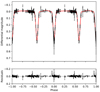 |
Fig. 1. Phase-folded light curve of M 3-2, assuming a period of 1.8767 days. The fit based on the parameters presented in Table 1 is indicated by the red curve. The differential magnitude was arbitrarily normalised. |
We model the light curve using the PHOEBE 2.0 code (Prša et al. 2016) using a Markov chain Monte Carlo (MCMC) method implemented via emcee (Foreman-Mackey et al. 2013) and parallelised to run on the LaPalma supercomputer with schwimmbad (Price-Whelan & Foreman-Mackey 2017). We allowed the masses, temperatures and radii of both stars as well as the orbital inclination to vary. The limb-darkening values for both stars were fixed to the default prescription in PHOEBE 2.0, whereby values for each point on the star are interpolated from tables derived from stellar atmosphere model emergent intensities calculated for 32 points along the stellar limb as described in Prša et al. (2016). A corner plot of the resulting MCMC chain for the varied parameters is shown in Fig. 2 while the parameters of the resulting fit are given in Table 1.
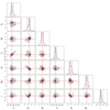 |
Fig. 2. A corner plot for the PHOEBE 2.0 MCMC fit to the light curve. Indicated are the temperature, radius and mass of the two stars, as well as the orbital inclination. The red lines represent the most likely values, while the dashed lines reflect the one-sigma limits. |
Best fit model of the binary system.
As can be seen from Fig. 1, the fit is very good, with the root mean square (rms) being of the order of 15 mmag. The eccentric orbit is confirmed, with a value of e = 0.149. Therefore, even if the orbital period is well within the range of observed and expected periods for close binary central stars of PNe, such a finite eccentricity is rather puzzling for the outcome of a common-envelope evolution, which should in most cases (if not always) lead to a circular orbit.
Given the lack of colour information provided by the single-band light curve, the individual temperatures of the two stars are relatively poorly constrained – with a strong correlation between the temperatures of the primary and the secondary. However, as implied directly from the similar eclipse depths, the stars are found to present extremely similar temperatures of around 8100–8200 K (corresponding to an A-type star). The radii and masses are slightly better constrained but, once again, show clear correlations between the two stars with the mass and radii ratios both being roughly unity. The inclination of the orbit is better constrained at i = 84.2∘.
3. Stellar spectroscopy
In order to better characterise the newly discovered binary system, we obtained on the night between 7 and 8 January, 2016, a spectrum of the central star, using FORS2 and the 300V grism, with a dispersion of 112 Å mm−1 and covering the wavelength range 3300–6600 Å, above which second-order contamination is present. The slit was aligned north-south, had a width of 0.7″ and the exposure time was 180 s. The seeing was about 0.8″, while the observations were done at airmass 2. The white dwarf GD50 was used as a spectrophotometric standard. The resulting spectrum is shown in Fig. 3. The obtained spectrum corresponds to an orbital phase of ϕ = 0.41 according to our ephemeris, meaning that it is out of eclipse.
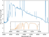 |
Fig. 3. FORS2 spectrum of the bright central star of M 3-2 taken with the 300V grism. No attempt was made to remove the nebular lines. The inset shows a zoom in the blue part of the spectrum, with a synthetic spectrum corresponding to a model of Teff = 8500 K, logg = 4.0 shown in orange. As the stellar spectrum is affected by the nebular lines, the bottom of the lines are not well fitted. |
Given the results from the light curve fitting, we have fitted the observed stellar spectrum assuming two similar objects, using the stellar spectral synthesis program SPECTRUM2 (Gray & Corbally 1994). We neglected here the extinction, as it is known to be very small (see below). In order to correctly fit the Balmer jump as well as the wings of the Balmer series, we find that models with effective temperatures of Teff= 8000–8500 K and gravity of logg = 4.0 − 4.5 are needed. This provides independent confirmation of our light curve analysis.
4. Nebular abundances
In addition to the stellar spectrum, we have also secured on the night between 6 and 7 January, 2016, a deep (1800 s) spectrum of the nebula of M 3-2 using FORS2, the same 300V grism, and same slit width of 0.7″ (Fig. 4). The seeing was also around 0.8″, the observations were done at airmass 1.3, and the slit was also oriented north-south. The same spectrophotometric standard star was used. The slit was placed in such a way as to avoid the bright star 3″ to the east.
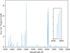 |
Fig. 4. FORS2 spectrum of the nebula of M 3-2 taken with the 300V grism, a 1″ wide slit and an exposure time of 1800 s. The right inset shows the [NII] and Hα lines, illustrating the strong nitrogen lines. |
From the ratio of Hα to Hβ, we derive an extinction c(Hβ) = 0.093 ± 0.069, giving A(V)=0.19. This value is in agreement with Kniazev (2012), who found c(Hβ) = 0.12 ± 0.05.
We used alfa (Wesson 2016) to fit the nebular lines and neat (Wesson et al. 2012) to determine the abundances of the chemical elements3. The effectiveness of alfa and neat in studying the physical and chemical properties of planetary nebulae from FORS2 spectroscopy has been well demonstrated in previous studies (e.g. Jones et al. 2016). Alfa optimises Gaussian fits to the observed emission lines using a genetic algorithm. The line fluxes thus measured are then passed to neat, which applies an empirical scheme to calculate the abundances. The calculations use a three-zone model of low, medium and high ionisation. Uncertainties are propagated through all steps of the analysis into the final values.
The resulting line intensities are shown in Table A.2 (available at the CDS), while the outcome of neat is shown in Table 2. Our results confirm the values obtained by Kniazev (2012), namely that the PN M 3-2 is a type I PN with a relatively low oxygen abundance but a high helium content. The logarithmic abundance of [O/H] is 7.8, considerably lower than the value of 8.54 found for a sample of PNe outside the solar circle (Wesson et al. 2005).
Output of neat abundance analysis of M 3-2.
5. Analysis: A clear case of false identity
The object that we observed, despite its projected position appearing close to the centre of the nebula, is most likely not the real central star of M 3-2. Indeed, as it consists of a close binary with an eccentric orbit containing two main sequence stars, of A or F spectral types, it cannot be the progenitor of the ionised nebula.
The fact that the bright object is not the real CSPN should not come as a surprise, though. First, it is obviously off-centre, although there are some other examples of PN with off-centre CSPN. Second, based on the Ambartsumyan (or “crossover”) temperature of the central star of 267 000 K, and given its distance, Kaler & Jacoby (1989) found that the hot central star of M 3-2 should have a V-magnitude of 23.36, well below the observed value, leading these authors to conclude that they had “clearly ...measured the bright companion of the true central star”. The same authors (Jacoby & Kaler 1989) seem to have found a much fainter star (V = 21.1) at the centre of the PN, ∼3″ from the bright central star. They measured its magnitude after removing the bright star by subtracting a scaled stellar profile from the image of the star.
To confirm this, we obtained deep images of the PN M 3-2 with FORS2 in both Hα and B-band, shown in Figs. 5 and A.2, respectively. While Fig. 5 clearly reveals the intricate nature of the nebula and its bipolar shape, Fig. A.2 allows us to detect a faint object next to the bright star we have been analysing until now. By doing a point spread function (PSF) fitting of the bright star and subtracting it from the image, a faint star at the very centre of the nebula is clearly visible (see Fig. 6) and is most likely the real CSPN, especially as it appears very blue (although its exact colours are rather uncertain due to the nebular contamination and possible remnant artefacts from the subtraction of the bright binary). The estimated brightness and location are provided in Table 3.
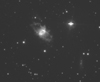 |
Fig. 5. M 3-2 in Hα observed with FORS2. The field of view is 2.4′×1.9′. North is up and east is to the right. |
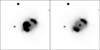 |
Fig. 6. Showing the likely CSPN after subtracting the bright object. |
Tylenda et al. (1991) measured the bright object to have magnitudes B = 16.53 and V = 16.31, presenting a colour excess B − V consistent with the range of temperatures derived by our light-curve modelling (Pickles 1998). Taking an absolute magnitude and bolometric V-band correction from Pickles (1998), the above-derived A(V)=0.2, and accounting for the fact that the observed apparent magnitude corresponds to the sum of both stars, implies a distance to the binary of approximately 8 kpc. Similarly, based on the comparison between our synthetic spectra and the flux calibrated FORS2 stellar spectrum, we are led to a ratio between the distance and the stellar radius of (d/R)=(2.75 ± 0.22)×1011. Given the radius determined from the light curve, this translates to a distance of 7.5 ± 0.6 kpc, depending on the effective temperature and gravity. This distance is well beyond the estimated one to the nebula, in most cases, between 3 and 5 kpc (see above), although it is compatible with some values provided in the literature. The binary system and the nebula are therefore most likely not linked, except by some unfortunate and distracting alignment. Given that the binary clearly does not contain the CSPN, we did not follow it sufficiently to derive the spectroscopic orbit and thus determine its systemic radial velocity. If done, this could be compared against the nebula’s velocity as an additional check. Based on our analysis of the nebular lines, the radial velocity of the PN is 66.7 ± 3.9 kms−1. If the binary and the nebula were linked, however, as the separation on sky is 2″, the physical separation would be ≈15, 000 au, making it a very wide, most likely unbound, hierarchical triple. We note that the Gaia DR2 release4 (Gaia Collaboration 2016, 2018) lists a star of G = 16.239 and colour Gp − Rp = 0.48 at the position of the bright star (α = 07 : 14 : 49.92; δ = −27 : 50 : 23.2; J2000). The parallax is, however, not very useful for now, being 0.0535 ± 0.0516 mas, but would be in line with a very distant object, and should, hopefully, be more precise in future data releases. Given its brightness, the real CSPN, though, will not be available in any future Gaia data releases.
Properties of the likely CSPN of PN M 3-2.
6. Discussion and conclusions
A photometric monitoring of the PN M 3-2 reveals the presence of an eclipsing close binary with an orbital period of 1.88 days in an eccentric orbit. Because close binary CSPNe are the result of common-envelope evolution – a strongly dissipative process – mostly circular orbits are expected, and this result is therefore at first sight very surprising. Furthermore, the light curve shows the presence of two almost equal eclipses, whose depth and duration imply the presence of stars with an almost solar radius size. Additional spectroscopy confirms that the components of the system are almost equal-mass main sequence stars, located about 8 kpc away. This is much farther than the estimated distance of the planetary nebula, showing that this binary is most likely just a chance superposition onto the true CSPN. The CSPN itself is much fainter, most likely located 2″ from the bright star and with an estimated B ∼ 20.3.
The mere existence of this alignment acutely illustrates the non-significance of using a statistical argument when disproving a chance alignment. The recent confirmation that the binary thought to be related to the CSPN of PN SuWt 2 is merely a field star system lying by chance in the same line of sight as the nebular centre, and that it bears no relation to SuWt 2, or its yet unidentified central star(s) (Jones & Boffin 2017), shows that this unfortunate circumstance now exists twice. We can try to crudely quantify this by querying SIMBAD for all stars listed as having spectral type A. This returns ≈100 000 stars in total. Subsequently, we assume a population of PNe of ≈3000. If two populations of objects of these sizes were uniformly distributed across the sky – a very crude approximation – then the probability that there is one chance alignment to within 10″ among the 3 × 10⁸ possible pairs of objects is 1.4%. The probability of two such alignments is just 0.02%. Of course, the fact that both A stars and PNe are strongly concentrated in the Galactic plane increases the chances of such alignments, but the occurrence of two is still remarkably unlikely.
Another estimate can be done using the Gaia DR2 catalogue. We have probed for all objects within 1 degree of the PN M 3-2 that are bright (G < 19) and blue (−0.1 < Bp − Rp < 0.5). We obtain 2476 possible sources. Doing the same for PN SuWt 2 returns 420 objects. Scaling the 1 degree field to a 10″ region leads to a 1.9% probability of a chance alignment around M 3-2 and 0.3% around SuWt 2. Assuming both are independent, the chance of having two alignments would be 0.006%, and therefore, given the 3000 known PNe, translates to less than 0.2 occurrences. We do know one such occurrence, however. It thus appears clear that nature likes to play tricks with us!
It is also worth mentioning that we also know of a few cases of superpositions of bright stars with bulge PNe (see, e.g., Appendix E of Miszalski et al. 2013a), many of which will have a similar distance of ∼8 kpc. The anonymous referee asks us to mention that these results raise the possibility that other binary central stars may, in fact, be misidentified field stars – particularly those in crowded fields (such as in the galactic bulge). However, this is mostly true for stars that have not been thoroughly studied, as in most cases the colours of the central stars should already provide confirmation of their nature. Moreover, whenever possible, radial velocities, UV/NIR photometry, spectroscopic peculiarities, and so on, can be used to establish an association (e.g. Miszalski et al. 2012, 2013b).
Given the clear bipolar nature of PN M 3-2, it seems likely that it contains a binary central star, and we encourage readers to try to prove this. Given the magnitude of the central star, however, this may be difficult. One way forward would be to use the link between close binarity and the abundance discrepancy factor (Wesson et al. 2018). These latter authors have found that central star binary periods are correlated with other observable parameters: considering the discrepancy between the recombination line and collisionally excited line abundances, extreme values (> 10) of this discrepancy are seen only where the binary period is less than about 1.15 days. These short periods and extreme abundance discrepancies are also associated with low-density (< 1000 cm−3) nebulae. In the case of M 3-2, our spectra are not deep enough to detect recombination lines of O2+, but we can place an upper limit to the abundance discrepancy factor (adf) of about 15. In addition, the density of the nebula is measured at ∼2000 cm−3 from [O II] lines and ∼5000 cm−3 from [Cl III] lines. While the upper limit to the adf is relatively weak, the density of M 3-2 is higher than any of the nebulae containing short-period binary central stars and an extreme adf. Therefore, the morphology of the nebula points to a short-period binary central star, while its chemistry and density further suggest that this binary should have a period longer than about 1.15 days.
See the latest list at http://drdjones.net/?q=bCSPN
SPECTRUM is available at http://www.appstate.edu/~grayro/spectrum/spectrum.html
Both software are available for download from https://github.com/rwesson
Acknowledgments
Part of this work was done while HMJB was visiting the IAC, thanks to a visitor grant in the framework of a Severo Ochoa excellence programme (SEV-2015-0548). This research made use of Astropy, a community-developed core Python package for Astronomy (Astropy Collaboration 2013, 2018), numpy (Van Der Walt et al. 2011), matplotlib (Hunter 2007) and corner (Foreman-Mackey 2016). This research has been supported by the Spanish Ministry of Economy and Competitiveness (MINECO) under the grant AYA2017-83383-P. The authors thankfully acknowledge the technical expertise and assistance provided by the Spanish Supercomputing Network (Red Española de Supercomputación), as well as the computer resources used: the LaPalma Supercomputer, located at the Instituto de Astrofísica de Canarias. B.M. acknowledges support from the National Research Foundation (NRF) of South Africa. This work was partially funded by the Spanish MINECO through project AYA2016-78994-P. RW was supported by European Research Grant SNDUST 694520. This work has made use of data from the European Space Agency (ESA) mission Gaia (https://www.cosmos.esa.int/gaia), processed by the Gaia Data Processing and Analysis Consortium (DPAC, https://www.cosmos.esa.int/web/gaia/dpac/consortium). Funding for the DPAC has been provided by national institutions, in particular the institutions participating in the Gaia Multilateral Agreement.
References
- Astropy Collaboration (Robitaille T. P., et al.) 2013, A&A, 558, A33 [NASA ADS] [CrossRef] [EDP Sciences] [Google Scholar]
- Astropy Collaboration (Price-Whelan A. M., et al.) 2018, AJ, 156, 123 [Google Scholar]
- Balick, B., & Frank, A. 2002, ARA&A, 40, 439 [NASA ADS] [CrossRef] [Google Scholar]
- Boffin, H. 2015a, 19th European Workshop on White Dwarfs (ASPC), 493, 527 [NASA ADS] [Google Scholar]
- Boffin, H. M. J. 2015b, Ecology of Blue Straggler Stars, eds. H. M. J. Boffin, G. Carraro, & G. Beccari (Springer), 153 [Google Scholar]
- Buzzoni, B., Delabre, B., Dekker, H., et al. 1984, ESO Messenger, 38, 9 [Google Scholar]
- Cahn, J. H., & Kaler, J. B. 1971, ApJS, 22, 319 [NASA ADS] [CrossRef] [Google Scholar]
- De Marco, O. 2009, PASP, 121, 316 [NASA ADS] [CrossRef] [Google Scholar]
- Foreman-Mackey, D. 2016, JOSS, 1, 24 [NASA ADS] [CrossRef] [Google Scholar]
- Foreman-Mackey, D., Hogg, D. W., & Lang, D. 2013, PASP, 125, 306 [CrossRef] [Google Scholar]
- Gaia Collaboration (Prusti, T., et al.) 2016, A&A, 595, A1 [NASA ADS] [CrossRef] [EDP Sciences] [Google Scholar]
- Gaia Collaboration (Brown, A. G. A., et al.) 2018, A&A, 616, A1 [NASA ADS] [CrossRef] [EDP Sciences] [Google Scholar]
- Gray, R. O., & Corbally, C. J. 1994, AJ, 107, 742 [NASA ADS] [CrossRef] [Google Scholar]
- Hunter, J. D. 2007, Comput. Sci. Eng., 9, 90 [Google Scholar]
- Jacoby, G. H., & Kaler, J. B. 1989, AJ, 98, 1662 [NASA ADS] [CrossRef] [Google Scholar]
- Jones, D., & Boffin, H. M. J. 2017a, Nat. Astron., 1, 117 [Google Scholar]
- Jones, D., & Boffin, H. M. J. 2017b, MNRAS, 466, 2034 [NASA ADS] [CrossRef] [Google Scholar]
- Jones, D., Boffin, H. M. J., Miszalski, B., et al. 2014, A&A, 562, A89 [NASA ADS] [CrossRef] [EDP Sciences] [Google Scholar]
- Jones, D., Boffin, H. M. J., Rodríguez-Gil, P., et al. 2015, A&A, 580, A19 [NASA ADS] [CrossRef] [EDP Sciences] [Google Scholar]
- Jones, D., Wesson, R., García-Rojas, J., et al. 2016, MNRAS, 455, 3263 [NASA ADS] [CrossRef] [Google Scholar]
- Kaler, J. B., & Jacoby, G. H. 1989, ApJ, 345, 871 [NASA ADS] [CrossRef] [Google Scholar]
- Kniazev, A. Y. 2012, Astron. Lett., 38, 707 [NASA ADS] [CrossRef] [Google Scholar]
- Maciel, W. J. 1984, A&AS, 55, 253 [NASA ADS] [Google Scholar]
- Minkowski, R. 1948, PASP, 60, 386 [NASA ADS] [CrossRef] [Google Scholar]
- Miszalski, B., Acker, A., Parker, Q. A., & Moffat, A. F. J. 2009, A&A, 505, 249 [NASA ADS] [CrossRef] [EDP Sciences] [Google Scholar]
- Miszalski, B., Boffin, H. M. J., Frew, D. J., et al. 2012, MNRAS, 419, 39 [NASA ADS] [CrossRef] [Google Scholar]
- Miszalski, B., Mikołajewska, J., & Udalski, A. 2013a, MNRAS, 432, 3186 [NASA ADS] [CrossRef] [Google Scholar]
- Miszalski, B., Boffin, H. M. J., Jones, D., et al. 2013b, MNRAS, 436, 3068 [NASA ADS] [CrossRef] [Google Scholar]
- Miszalski, B., Manick, R., Mikołajewska, J., et al. 2018, PASA, 35, e027 [NASA ADS] [CrossRef] [Google Scholar]
- Phillips, J. P. 2004, MNRAS, 353, 589 [NASA ADS] [CrossRef] [Google Scholar]
- Pickles, A. J. 1998, PASP, 110, 863 [CrossRef] [Google Scholar]
- Price-Whelan, A., & Foreman-Mackey, D. 2017, JOSS, 2, 375 [Google Scholar]
- Prša, A., Conroy, K. E., Horvat, M., et al. 2016, ApJS, 227, 29 [NASA ADS] [CrossRef] [Google Scholar]
- Shaw, R. A., & Kaler, J. B. 1989, ApJS, 69, 495 [NASA ADS] [CrossRef] [Google Scholar]
- Shortridge, K., Meyerdierks, H., Currie, M. J., et al. 2004, Starlink User Note 86.21 (Rutherford Appleton Laboratory) [Google Scholar]
- Tylenda, R., Acker, A., Raytchev, B., et al. 1991, A&AS, 89, 77 [NASA ADS] [Google Scholar]
- Van Der Walt, S., Colbert, S. C., & Varoquaux, G. 2011, Comput. Sci. Eng., 13, 22 [CrossRef] [Google Scholar]
- Wesson, R. 2016, MNRAS, 456, 3774 [NASA ADS] [CrossRef] [Google Scholar]
- Wesson, R., Liu, X.-W., & Barlow, M. J. 2005, MNRAS, 362, 424 [NASA ADS] [CrossRef] [Google Scholar]
- Wesson, R., Stock, D. J., & Scicluna, P. 2012, MNRAS, 422, 3516 [NASA ADS] [CrossRef] [Google Scholar]
- Wesson, R., Jones, D. García-Rojas, J., et al. 2018, MNRAS, 480, 4589 [NASA ADS] [CrossRef] [Google Scholar]
Appendix A: Additional figures
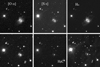 |
Fig. A.1. EFOSC2 images of M 3-2 in different narrow-band (top) and broadband (bottom) filters. North is up and east is to the left. |
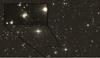 |
Fig. A.2. Showing the likely CSPN with FORS2, with a deep image in B. The intensity is shown with a logarithmic scale and the upper inset shows a zoom-in around the PN. The arrow indicates the real CSPN. |
All Tables
All Figures
|
Fig. 1. Phase-folded light curve of M 3-2, assuming a period of 1.8767 days. The fit based on the parameters presented in Table 1 is indicated by the red curve. The differential magnitude was arbitrarily normalised. |
| In the text | |
|
Fig. 2. A corner plot for the PHOEBE 2.0 MCMC fit to the light curve. Indicated are the temperature, radius and mass of the two stars, as well as the orbital inclination. The red lines represent the most likely values, while the dashed lines reflect the one-sigma limits. |
| In the text | |
|
Fig. 3. FORS2 spectrum of the bright central star of M 3-2 taken with the 300V grism. No attempt was made to remove the nebular lines. The inset shows a zoom in the blue part of the spectrum, with a synthetic spectrum corresponding to a model of Teff = 8500 K, logg = 4.0 shown in orange. As the stellar spectrum is affected by the nebular lines, the bottom of the lines are not well fitted. |
| In the text | |
|
Fig. 4. FORS2 spectrum of the nebula of M 3-2 taken with the 300V grism, a 1″ wide slit and an exposure time of 1800 s. The right inset shows the [NII] and Hα lines, illustrating the strong nitrogen lines. |
| In the text | |
|
Fig. 5. M 3-2 in Hα observed with FORS2. The field of view is 2.4′×1.9′. North is up and east is to the right. |
| In the text | |
|
Fig. 6. Showing the likely CSPN after subtracting the bright object. |
| In the text | |
|
Fig. A.1. EFOSC2 images of M 3-2 in different narrow-band (top) and broadband (bottom) filters. North is up and east is to the left. |
| In the text | |
|
Fig. A.2. Showing the likely CSPN with FORS2, with a deep image in B. The intensity is shown with a logarithmic scale and the upper inset shows a zoom-in around the PN. The arrow indicates the real CSPN. |
| In the text | |
Current usage metrics show cumulative count of Article Views (full-text article views including HTML views, PDF and ePub downloads, according to the available data) and Abstracts Views on Vision4Press platform.
Data correspond to usage on the plateform after 2015. The current usage metrics is available 48-96 hours after online publication and is updated daily on week days.
Initial download of the metrics may take a while.