| Issue |
A&A
Volume 619, November 2018
|
|
|---|---|---|
| Article Number | A102 | |
| Number of page(s) | 6 | |
| Section | Stellar structure and evolution | |
| DOI | https://doi.org/10.1051/0004-6361/201833274 | |
| Published online | 12 November 2018 | |
Nebular spectroscopy of SN 2014J: Detection of stable nickel in near-infrared spectra
1
Oskar Klein Centre, Department of Physics, Stockholm University, 106 91 Stockholm, Sweden
e-mail: suhail.dhawan@fysik.su.se
2
European Southern Observatory, Karl-Schwarzschild-Strasse 2, 85748 Garching bei München, Germany
3
Max-Planck-Institut für Astrophysik, Karl-Schwarzschild-Straße 1, 85748 Garching bei München, Germany
4
Physik-Department, Technische Universität München, James-Franck-Straße 1, 85748 Garching bei München, Germany
5
Excellence Cluster Universe, Technische Universität München, Boltzmannstraße 2, 85748 Garching, Germany
6
Astrophysics Research Centre, School of Mathematics and Physics, Queen’s University Belfast, Belfast BT7 1NN, UK
7
Department of Astronomy and Astrophysics, University of Toronto, 50 St. George Street, Toronto ON M5S 3H4, Canada
Received:
20
April
2018
Accepted:
24
July
2018
We present near-infrared (NIR) spectroscopy of the nearby supernova 2014J obtained ∼450 d after explosion. We detect the [Ni II] 1.939 μm line in the spectra indicating the presence of stable 58Ni in the ejecta. The stable nickel is not centrally concentrated but rather distributed as the iron. The spectra are dominated by forbidden [Fe II] and [Co II] lines. We used lines, in the NIR spectra, arising from the same upper energy levels to place constraints on the extinction from host galaxy dust. We find that that our data are in agreement with the high AV and low RV found in earlier studies from data near maximum light. Using a 56Ni mass prior from near maximum light γ-ray observations, we find 0.053 ± 0.018 M⊙ of stable nickel to be present in the ejecta. We find that the iron group features are redshifted from the host galaxy rest frame by ∼600 km s−1.
Key words: supernovae: individual: SN 2014J / supernovae: general
© ESO 2018
1. Introduction
Type Ia supernovae (SNe Ia) have long been identified as thermonuclear explosions of C/O white dwarfs (WD; Hoyle & Fowler 1960). Following a simple calibration (Phillips 1993) they are excellent distance indicators used extensively in cosmology (Riess et al. 1998; Perlmutter et al. 1999). There remain several open questions regarding the physics of SNe Ia, for example progenitor channel, mass of the progenitor, explosion mechanism, (see Hillebrandt & Niemeyer 2000; Leibundgut 2001; Hillebrandt et al. 2013; Maoz et al. 2014; Wang 2018; Livio & Mazzali 2018, for reviews). Many attempts to address these issues have concentrated on photometric and spectroscopic observations of SNe Ia near maximum light (i.e. the photospheric phase). However, at late times, as the ejecta become optically thin and the core of the ejecta is revealed, additional diagnostics of the explosion mechanism become accessible. The elegance of SNe Ia lies in the fact that both the energy of the explosion and the electromagnetic display are due to the burning of the core to 56Ni and its subsequent decay. Direct or indirect measurements of the mass and topology of 56Ni provide some of the best probes of the explosion physics. The decay of 56Ni to 56Co and on to stable 56Fe proceeds through the emission of γ-rays and positrons which power the electromagnetic display.
Nebular phase spectroscopy enables a direct view into the core of the ejecta and provides key insights into the progenitor and explosion properties of SNe Ia, complementary to the early time observations which contain information about the outer layers of the ejecta. The evolution of the cobalt to iron line ratios in nebular spectra have been used to demonstrate radioactive decay as the mechanism powering SNe Ia (Kuchner et al. 1994) and a combination of optical and near-infrared (NIR) spectra have provided constraints on the iron mass in the ejecta (Spyromilio et al. 1992, 2004). Moreover, correlations of nebular-phase line velocities with photospheric-phase velocity gradients have indicated asymmetries in the explosion mechanism (Maeda et al. 2010a,b; Maguire et al. 2018). Most nebular-phase studies of SNe Ia (e.g. Silverman et al. 2013; Graham et al. 2017) have concentrated on optical wavelengths. Since the iron and cobalt features in the NIR are relatively unblended compared to the optical, it is an interesting wavelength region to study the line profiles. Some studies use the [Fe II] 1.644 μm feature to probe the kinematic distribution of the radioactive ejecta (Höflich et al. 2004; Motohara et al. 2006) and have also tried to constrain the central density and magnetic field of the progenitor WD (Penney & Hoeflich 2014; Diamond et al. 2015). Gerardy et al. (2007) use mid-infrared nebular spectra to explore the explosion mechanism and electron capture elements.
The presence of large amounts of stable isotopes of nickel (e.g. 58Ni and 60Ni) has been suggested as an indicator of burning at high central densities and therefore would favour higher progenitor masses, contributing to evidence for a Chandrasekhar-mass progenitor scenario for some supernovae (Höflich et al. 2004). SN 2014J in M82 is one of the nearest SN Ia in decades and has been extensively studied (e.g. Kelly et al. 2014; Diehl et al. 2014; Foley et al. 2014; Ashall et al. 2014; Vacca et al. 2015; Galbany et al. 2016; Vallely et al. 2016). It is heavily reddened by host galaxy dust, but shows spectral features of a normal SN Ia (Amanullah et al. 2014). The extinction law and properties of the dust along the line of sight have been extensively discussed by a number of authors (Kawabata et al. 2014; Foley et al. 2014; Goobar et al. 2014).Imagingof the supernova reveals the presence of clear echoes (Yang et al. 2017). Estimates of the 56Ni mass using the timing of the NIR second maximum (Dhawan et al. 2016) and γ-ray observations (Churazov et al. 2015) infer masses of 0.64 ± 0.13 M⊙ and 0.62 ± 0.13 M⊙, respectively, consistent with mid-infrared spectra (Telesco et al. 2015) and the estimate for a normal SN Ia (Stritzinger et al. 2006; Scalzo et al. 2014). Optical spectra of SN 2014J in the nebular phase are remarkably similar to the “normal” SNe 2011fe and 2012cg (Amanullah et al. 2015).
In this work we present the first detection of a spectral line at 1.939 μm in an SN Ia, a forbidden [Ni II] transition (4F9/2–2F7/2), indicating the presence of stable nickel isotopes (e.g., see Wilk et al. 2018). We use the ratios of the [Fe II] lines to measure the parameters describing the host galaxy extinction and evaluate the line shifts and profiles for the spectra. We present the data in Sect. 2, analyse them in Sect. 3, discuss our results in Sect. 4 and conclude in Sect. 5.
Observing log of spectra obtained with GNIRS on the Gemini-North telescope.
2. Observations and data reduction
SN 2014J was discovered in M 82 at the University of London Observatory on Jan 21st 2014 (Fossey et al. 2014). We adopt MJD 56671.7 as the epoch of explosion (Goobar et al. 2014). We present NIR spectra of SN 2014J, obtained using GNIRS on Gemini-North. The dates and phases are shown in Table 1. The observations were made using the Gemini fast turnaround programme (Mason et al. 2014) under proposal GN-2015A-FT-3. The spectra were obtained in cross-dispersed (XD) mode with a central wavelength of 1.65 μm and have a wavelength coverage from 0.825 to 2.5 μm.
The spectra were reduced using the standard Gemini IRAF1 package. The final spectra were extracted using the IRAF task apall which extracts one-dimensional sums across the apertures. For the first epoch (March) we used the A0 star HIP 32549 from the Gemini archive (not observed on the same night) for telluric correction but we are unable to colour correct our data since no suitable standard on the same night was observed. The March spectrum is therefore only used for measurements of line shifts and profiles but not for line ratios. For the second (April) and third (May) epochs, we use the A7 star HIP 50685 obtained on the same nights as the observations of the supernova for both telluric and spectrophotometric calibration. Given that the features we are studying lie in regions of variable atmospheric transmission, we have checked our standard star observations against atmospheric transmission models of the atmosphere. We find that the transmission of the standard star is compatible with the Mauna Kea atmospheric models from the Gemini web site2 for 50 mm of water vapour and an airmass of 2.0. The individual features of the atmosphere are reproduced well by the spectrum at the appropriate instrumental resolution.
No discernible continuum is present in the J and H bands in any of our data. In the K band we cannot exclude the presence of an underlying continuum although this may have an instrumental contibution as well as an astronomical one. The spectra are shown in Fig. 1.
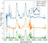 |
Fig. 1. NIR spectra of SN 2014J (for the three nights it was observed). The spectra are plotted in mJy for visibility and each spectrum is incrementally displaced vertically by 2 mJy. The March data are at top and the May data at the bottom. The regions of poor atmospheric transmission around 1.4 and 1.9 μm are clearly identifiable due to the increased noise. The inset shows the region between 1.85 and 2.03 μm (the expected region for the [Ni II] feature) in the March spectrum. |
3. Analysis
3.1. Nickel detection
In our data (see Fig. 1), we note the presence of a weak line at a wavelength coincident with the central wavelength of a [Ni II] transition. In Fig. 2 we fit the feature and present the first clear detection of the 4F9/2–2F7/2 [Ni II] 1.939 μm line in the spectra of a Type Ia supernova. Since the e-folding timescale of radioactive nickel is 8.8 d (Nadyozhin 1994) and the spectra are taken at ∼450 d, this implies that the detection of the [Ni II] line indicates the presence of stable nickel.
In our spectra there is no evidence for the 2D5/2–4F7/2 line of [Ni II] at 1.0718 μm, which has an A value two orders of magnitude lower than the 1.939 μm line. Our modelling of the atmospheric transmission and the standard star spectra suggest that, if the line were strong, we should observe the centre of the line and the blue wing. Given the extinction and our assumed excitation conditions (see Sect. 3.2) we cannot use the absence of a strong line at 1.0718 μm to challenge the identification of the 1.939 μm line.
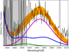 |
Fig. 2. Spectrum taken in May and a model using an [Ni II] NLTE atom (magenta) with a line width of 11 000 (±2100) km s−1 redshifted by 800 km s−1 from the laboratory rest frame. In the 1.8–2 μm region weak [Fe II] lines (blue) and [Co II] lines (green) are also present. Shortwards of the central wavelength of this line the transmission is low and the noise in the spectrum increases (grey shaded region). This region has not been used in the fitting algorithm. |
3.2. Fitting the spectrum
The NIR spectrum of SN 2014J is dominated by forbidden lines of singly ionised iron and singly ionised cobalt. In particular the prominent features at the long end of the J window (around 1.26 μm) and most of the H-band emission arise from multiplets a6D–a4D and a4F–a4D of [Fe II], respectively, while the feature around 0.86 μm has contributions from the [Fe II] a4F–a4P multiplet and from [Co II] a3F–b3F. Additional contributions from [Co II] a5F–b3F are present in the H band (at 1.547 μm). The line identification is provided in Table 2.
Fitting the J and H band spectra is relatively straightforward. The K band is very faint but the transitions in the K band are not expected to be strong. The model we use (Flörs et al. 2018) uses NLTE excitation of singly and doubly ionised iron group elements. For the purposes of fitting only the NIR data, the only contributing features are from the singly ionised species (which we input a priori) and a one zone model, convolved with a Gaussian line profile (which encapsulates the information about the energy deposition and the density profile), suffices to provide an excellent fit. The atomic data for our NLTE models are from Storey et al. (2016), Nussbaumer & Storey (1988, 1980), and Cassidy et al. (2010). The free parameters are the electron density and temperature of the gas, the ratio of iron to cobalt to nickel, the line widths, the offset from the systemic velocity of the supernova that the singly ionised transitions of the iron group elements may exhibit and the extinction. We explore the parameter space with the nested-sampling algorithm Nestle3 and a χ2 likelihood. Uniform priors are used for all parameters except the electron density. For this we assume a lower bound of 105 cm−3. As has also been observed for other SN Ia at this epoch, our spectrum shows no evidence for neutral iron lines. The strong lines of the [Fe I] a5D–a5F multiplet at 1.4 μm are in a poor transmission region but still remain undetected. The lowest-excitation and therefore presumably strongest [Fe I] line in the 2 μm region at 1.9804 μm from multiplet a5F–a3F is also not seen. The infrared spectrum provides some evidence in the K band for doubly ionised iron but it is well known from combined optical and infrared spectra (e.g. Spyromilio et al. 1992) that strong transitions of [Fe III] and [Co III] are present in the 4000–6000 Å region. As discussed in the introduction, from earlier work (Churazov et al. 2015; Dhawan et al. 2016) it has been determined that SN 2014J made ≈0.6 M⊙ of 56Ni. A simple distribution of this mass of Nickel and its daughter elements in singly ionised state in a volume expanding for the age of the supernova at 8000 km s−1 sets the electron density to be at least 105 cm−3.
The fits are shown in Fig. 3. Additional constraints arise from a few higher excitation lines in the 8600 Å region but these are extremely sensitive to the choice of atomic data. For the purposes of this work we note that we can fit these lines and that the fits are consistent with our derived properties but we do not draw conclusions based on this aspect of our data.
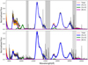 |
Fig. 3. Fits to the observations using a NLTE one zone emission code. Top: April and bottom: May spectra. The red lines indicate the mean model. The orange shaded band shows the 95% credibility region. Ion contributions are shown in blue ([Fe II]), green ([Co II]) and magenta ([Ni II]). The atmospheric absorption bands shortwards of 1.12, 1.48 and 1.915 μm are shaded grey. The resulting values for the temperature and electron density for April spectrum are 3700 ± 400 K and 2.18 (±0.56) × 105 cm−3 and 3300 ± 200 K and 1.69 (±0.59) × 105 cm−3. |
Dominant line identifications for SN 2014J.
3.3. Extinction
The two strongest lines in the spectrum are the [Fe II] 1.257 μm a6D9/2–a4D7/2 and the 1.644 μm [Fe II] a4F9/2–a4D7/2 which arise from the same upper level. In the absence of additional contributions to the features at these wavelengths and optical depth effects the observed line ratio and can be used to determine the extinction between the J and H bands as it depends solely on the Einstein A-values of these transitions. Additional constraints, independent of the excitation conditions come from the [Co II] lines at 1.547 μm (a5F4–b3F4) and 1.0191 μm (a3F4–b3F4) which also come from the same upper level. From our model fits of these features we can ensure that blending is taken consistently into account. We constrain the Cardelli et al. (1989) prescription for the extinction in the range shown in Fig. 4. The NIR data are compatible with both high and low values of RV. The degeneracy between AV and RV arises from the short wavelength lever arm between the J and H windows.
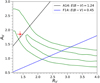 |
Fig. 4. Distribution for RV and AV values by fitting the [Fe II] lines (the contours shown here are for the April spectrum, the results for the May spectrum are consistent with the contours displayed here). The values measured by Amanullah et al. (2014) are marked in red and agree with our April spectrum. The contours mark the 1 and 2σ credible regions of the MCMC samples. The lines show a constant E(B – V) of 1.37 as derived by Amanullah et al. (2014) and a constant E(B – V) of 0.45 as derived by Foley et al. (2014). |
3.4. Line shifts and widths
As noted by Maeda et al. (2010b) some type Ia supernovae exhibit a shift of the line centres of the singly ionised iron group lines relative to the systemic velocity of the supernova and also with respect to the doubly ionised features, which they interpret as a signature of explosion asymmetry. In the absence of doubly ionised features in our data we cannot identify a differential velocity shift, only a shift of the singly ionised iron group lines relative to the host galaxy recession velocity. The velocity shift and the line width of the singly ionised lines are free parameters in the fit to the observed spectra, and the shift is calculated from the emission line spectrum, broadened by the fitted line width. We obtain a ∼800 km s−1 redshift for lines, from our fit, which is ∼600 km s−1 in excess of the M 82 recession velocity (assuming that the SN does not have any relative motion to its host galaxy). The [Ni II], [Co II] and [Fe II] lines exhibit the same shifts within the errors, although the constraint on the [Ni II] is weak and degenerate with the width.
The profiles of the iron and cobalt lines are well fit by a simple Gaussian line shape for each individual component of the multiplets. We find that a Full Width Half Maximum of 8600 ± 150 km s−1 fits the [Fe II] and [Co II] data.
The [Ni II] line width is 11 000 (±2100) km s−1, somewhat higher than but consistent within the errors with the iron and cobalt line widths. It is thus clear that the stable iron group elements are not at the lowest velocities, unlike the predictions from 1D Mch models. However, we find that the model predictions from 3D delayed detonation explosions of Seitenzahl et al. (2013) which predict stable isotopes at intermediate velocities are consistent with our observations. The somewhat higher velocity of the Nickel may be an artefact of our continuum placement which has been conservatively assumed to be non-existent. A small residual continuum, possibly from incomplete background subtraction, would result in the [Ni II] velocity being consistent with the other lines (see Sect. 3.2).
4. Discussion
Wilk et al. (2018) argued that the [Ni II] 1.939 μm line is relatively unblended compared to the strong [Ni II] feature at 7378 Å in the optical and therefore a more suitable test for the presence of large amounts of stable Nickel. Wilk et al. (2018) used models of Blondin et al. (2013, 2017) to model the optical and NIR spectra in the nebular regime.
That study (see Wilk et al. 2018, Fig. 13) shows a dramatic variation in the strength of the 1.939 μm line for their models, however, we note that their synthetic spectra are at epochs ∼200 d before the spectra presented here. The mass of stable nickel, however, in the models of Wilk et al. (2018), only varies by a factor of 3 between the different models used (∼0.011–0.03 M⊙). Compared to their yields, the Mch models of Seitenzahl et al. (2013) are slightly higher in the range between 0.03 and 0.07 M⊙. The appearance of the spectrum is particularly sensitive to the ionisation conditions in the models and therefore the derivation of masses from lines arising from a single ionisation stage, such as we have attempted here, is challenging. Our confirmation of the presence of the 1.939 μm line, which arises from the same upper level as the 7378 Å line confirms the identification of [Ni II] by Maguire et al. (2018).
4.1. Ionisation and masses of Fe+ and Ni+
From our fitting we determine an un-blended flux for 1.644 μm line and infer the mass of the emitting iron. For a distance to M 82 of 3.5 Mpc (Karachentsev & Kashibadze 2006) and our measured flux for the 1.644 μm line we determine a mass of ∼0.18 M⊙ for Fe+ at the epoch of the SN spectrum. We note that without the high density prior from the 56Ni mass, our spectra allow for low densities and high excitation conditions which can give Fe+ yields as low as 0.01 M⊙ (the masses reported here are the weighted mean for the +450 and +478 d spectra).
We note the strength of the 1.533 μm a4F9/2–a4D5/2 line and the presence of a blue shoulder at the 1.644 μm feature (at 1.6 μm) due to the a4F7/2–a4D3/2 [Fe II] line at 1.599 μm. The ratios of these lines to the 1.644 μm line are sensitive to the electron density, and the 1.54 μm feature as well as the shoulder drop for electron densities below 105 cm−3 (see also Nussbaumer & Storey 1988). Here again we have avoided placing a disproportionate weight on a particular feature in our likelihood function. We only note that this presents corroborating evidence for high electron densities, consistent with the inference on the density from the 56Ni mass prior, hence increasing our confidence in the Fe+ mass determination.
Using the derived mass of Fe+, the total iron mass prior and assuming that only the singly and doubly ionised species are present, we get an ionisation fraction of ≈2.3. This value is consistent with calculations from theory (∼1.6–2) in the literature (e.g. Axelrod 1980).
We can now proceed to derive a value of 0.016 ± 0.005 M⊙ for the Ni+ mass based on the emissivity of the 1.939 μm line and the other derived parameters from our fits. Similarly, assuming that all the Ni exists in singly and doubly ionised state and that ionisation fractions for nickel are the same as for iron (see Wilk et al. 2018, for caveats) then we estimate that approximately 0.053 ± 0.018 M⊙ of stable nickel is present in SN 2014J. While this is higher than the predictions for the different models, it is within 3σ of the predicted range of estimates.
We observed a complex of weak [Fe III] lines in the K-band. Using the Fe++ mass derived above (0.42 M⊙), the distance to M 82 (3.5 Mpc) and the observed flux in the region between 21 000 and 24 000Å (0.75 ± 0.2 × 10⁻¹⁴ erg s−1 cm−2) we derive an emissivity of ∼2 × 10⁻¹⁸ erg s−1 atom−1. This is consistent with the derived line emissivity from the NLTE calculations with a temperature of 4000 K and Ne of 105 cm−3. However, these estimates are highly sensitive to the temperature and Ne values, placement of the continuum and hence, only offer a consistency check.
4.2. Extinction by host galaxy dust
Measurements from maximum light photometry would point to a high E(B – V) (1.37 mag, see Amanullah et al. 2014). The authors find a non-standard reddening law describing the colour excesses at maximum light. Fitting a Cardelli et al. (1989) reddening law the authors also find a preference for RV ∼1.4, significantly smaller than the typical Milky Way value of 3.1. This is confirmed by spectro-polarimetry data in Patat et al. (2015), who also demonstrate the preference for low RV in other highly reddened SNe Ia, a trend that has been observed with multi-band observations of large samples of nearby SNe (Nobili & Goobar 2008; Phillips et al. 2013; Burns et al. 2014). The low RV would indicate smaller dust grains in the host of SN 2014J than in the Milky Way. UV spectrophotometry (Brown et al. 2015), the wavelength independence of the polarisation angle (Patat et al. 2015) and modelling the optical light curves (Bulla et al. 2018) point towards an interstellar origin of the dust. We note however, that Foley et al. (2014) find that a mixture of typical dust in a combination of interstellar reddening and circumstellar scattering provides good fits to the early multi-wavelength data. For this case an RV of 2.6 is derived by Foley et al. (2014). We find that the extinction derived from our NIR spectra using the [Fe II] and [Co II] line ratios is compatible with maximum light estimates for the reddening.
5. Conclusions
In this study we have presented NIR spectra of SN 2014J in the nebular phase. The dominant component of these spectra are [Fe II] and [Co II] lines. We detect, for the first time, a [Ni II] line at 1.939 μm, confirming the presence of stable nickel isotopes. We note that Friesen et al. (2014) suggest that a line at ∼1.98 μm in transitional phase (∼100 d) NIR spectra could be a [Ni II], however, the velocity shift of the feature is very high making it unlikely that it is due to [Ni II]. The [Fe II] and [Co II] lines are Gaussian with a width of 8600 km s−1 whereas the [Ni II] lines are at least as wide and possibly wider at 11 000 (±) 2100 km s−1. This indicates that the stable nickel is likely not at low velocities but rather at intermediate velocities, as predicted by multi-D Mch models. Our line profiles show no evidence for flat-top or belly-top like shapes (e.g. Penney & Hoeflich 2014; Diamond et al. 2015, 2018). The host galaxy extinction has been estimated from the NIR [Fe II] line ratios and is seen to be consistent with the inference from near-maximum photometry and polarimetry. Combining our spectral modelling with a prior on the 56Ni mass from maximum light and γ-ray observations, we obtain a mass of stable nickel of 0.053 ± 0.018 M⊙.
Acknowledgments
We would like to thank the staff at Gemini-North, especially Tom Geballe and Rachel Mason for their help during the observations and data reduction. BL and ST acknowledge support by TRR33 “The Dark Universe” of the German Research Foundation. KM acknowledges support from the UK STFC through an Ernest Rutherford Fellowship.
References
- Amanullah, R., Goobar, A., Johansson, J., et al. 2014, ApJ, 788, L21 [NASA ADS] [CrossRef] [Google Scholar]
- Amanullah, R., Johansson, J., Goobar, A., et al. 2015, MNRAS, 453, 3300 [NASA ADS] [CrossRef] [Google Scholar]
- Ashall, C., Mazzali, P., Bersier, D., et al. 2014, MNRAS, 445, 4427 [NASA ADS] [CrossRef] [Google Scholar]
- Axelrod, T. S. 1980, PhD Thesis, California Univ., Santa Cruz, USA [Google Scholar]
- Blondin, S., Dessart, L., Hillier, D. J., & Khokhlov, A. M. 2013, MNRAS, 429, 2127 [NASA ADS] [CrossRef] [Google Scholar]
- Blondin, S., Dessart, L., Hillier, D. J., & Khokhlov, A. M. 2017, MNRAS, 470, 157 [NASA ADS] [CrossRef] [Google Scholar]
- Brown, P. J., Smitka, M. T., Wang, L., et al. 2015, ApJ, 805, 74 [NASA ADS] [CrossRef] [Google Scholar]
- Bulla, M., Goobar, A., Amanullah, R., Feindt, U., & Ferretti, R. 2018, MNRAS, 473, 1918 [NASA ADS] [CrossRef] [Google Scholar]
- Burns, C. R., Stritzinger, M., Phillips, M. M., et al. 2014, ApJ, 789, 32 [NASA ADS] [CrossRef] [Google Scholar]
- Cardelli, J. A., Clayton, G. C., & Mathis, J. S. 1989, ApJ, 345, 245 [NASA ADS] [CrossRef] [Google Scholar]
- Cassidy, C. M., Ramsbottom, C. A., Scott, M. P., & Burke, P. G. 2010, A&A, 513, A55 [NASA ADS] [CrossRef] [EDP Sciences] [Google Scholar]
- Churazov, E., Sunyaev, R., Isern, J., et al. 2015, ApJ, 812, 62 [NASA ADS] [CrossRef] [Google Scholar]
- Dhawan, S., Leibundgut, B., Spyromilio, J., & Blondin, S. 2016, A&A, 588, A84 [NASA ADS] [CrossRef] [EDP Sciences] [Google Scholar]
- Diamond, T. R., Hoeflich, P., & Gerardy, C. L. 2015, ApJ, 806, 107 [NASA ADS] [CrossRef] [Google Scholar]
- Diamond, T. R., Hoeflich, P., Hsiao, E. Y., et al. 2018, ApJ, 861, 119 [NASA ADS] [CrossRef] [Google Scholar]
- Diehl, R., Siegert, T., Hillebrandt, W., et al. 2014, Science, 345, 1162 [NASA ADS] [CrossRef] [Google Scholar]
- Flörs, A., Spyromilio, J., Maguire, K., et al. 2018, A&A, in press, DOI: 10.1051/0004-6361/201833512 [Google Scholar]
- Foley, R. J., Fox, O. D., McCully, C., et al. 2014, MNRAS, 443, 2887 [NASA ADS] [CrossRef] [Google Scholar]
- Fossey, S. J., Cooke, B., Pollack, G., Wilde, M., & Wright, T. 2014, Central Bureau Electronic Telegrams, 3792 [Google Scholar]
- Friesen, B., Baron, E., Wisniewski, J. P., et al. 2014, ApJ, 792, 120 [NASA ADS] [CrossRef] [Google Scholar]
- Galbany, L., Moreno-Raya, M. E., Ruiz-Lapuente, P., et al. 2016, MNRAS, 457, 525 [NASA ADS] [CrossRef] [Google Scholar]
- Gerardy, C. L., Meikle, W. P. S., Kotak, R., et al. 2007, ApJ, 661, 995 [NASA ADS] [CrossRef] [Google Scholar]
- Goobar, A., Johansson, J., Amanullah, R., et al. 2014, ApJ, 784, L12 [NASA ADS] [CrossRef] [Google Scholar]
- Graham, M. L., Kumar, S., Hosseinzadeh, G., et al. 2017, MNRAS, 472, 3437 [NASA ADS] [CrossRef] [Google Scholar]
- Hillebrandt, W., & Niemeyer, J. C. 2000, ARA&A, 38, 191 [NASA ADS] [CrossRef] [Google Scholar]
- Hillebrandt, W., Kromer, M., Röpke, F. K., & Ruiter, A. J. 2013, Front. Phys., 8, 116 [NASA ADS] [CrossRef] [Google Scholar]
- Höflich, P., Gerardy, C. L., Nomoto, K., et al. 2004, ApJ, 617, 1258 [NASA ADS] [CrossRef] [Google Scholar]
- Hoyle, F., & Fowler, W. A. 1960, ApJ, 132, 565 [NASA ADS] [CrossRef] [EDP Sciences] [Google Scholar]
- Karachentsev, I. D., & Kashibadze, O. G. 2006, Astrophysics, 49, 3 [NASA ADS] [CrossRef] [Google Scholar]
- Kawabata, K. S., Akitaya, H., Yamanaka, M., et al. 2014, ApJ, 795, L4 [NASA ADS] [CrossRef] [Google Scholar]
- Kelly, P. L., Fox, O. D., Filippenko, A. V., et al. 2014, ApJ, 790, 3 [NASA ADS] [CrossRef] [Google Scholar]
- Kuchner, M. J., Kirshner, R. P., Pinto, P. A., & Leibundgut, B. 1994, ApJ, 426, 89 [NASA ADS] [CrossRef] [Google Scholar]
- Leibundgut, B. 2001, ARA&A, 39, 67 [NASA ADS] [CrossRef] [Google Scholar]
- Livio, M., & Mazzali, P. 2018, Phys. Rep., 736, 1 [NASA ADS] [CrossRef] [Google Scholar]
- Maeda, K., Benetti, S., Stritzinger, M., et al. 2010a, Nature, 466, 82 [NASA ADS] [CrossRef] [PubMed] [Google Scholar]
- Maeda, K., Taubenberger, S., Sollerman, J., et al. 2010b, ApJ, 708, 1703 [NASA ADS] [CrossRef] [Google Scholar]
- Maguire, K., Sim, S. A., Shingles, L., et al. 2018, MNRAS, 477, 3567 [NASA ADS] [CrossRef] [Google Scholar]
- Maoz, D., Mannucci, F., & Nelemans, G. 2014, ARA&A, 52, 107 [NASA ADS] [CrossRef] [Google Scholar]
- Mason, R. E., Côté, S., Kissler-Patig, M., et al. 2014, in Observatory Operations: Strategies, Processes, and Systems V, Proc. SPIE, 9149, 914910 [CrossRef] [Google Scholar]
- Motohara, K., Maeda, K., Gerardy, C. L., et al. 2006, ApJ, 652, L101 [NASA ADS] [CrossRef] [Google Scholar]
- Nadyozhin, D. K. 1994, ApJS, 92, 527 [NASA ADS] [CrossRef] [Google Scholar]
- Nobili, S., & Goobar, A. 2008, A&A, 487, 19 [NASA ADS] [CrossRef] [EDP Sciences] [Google Scholar]
- Nussbaumer, H., & Storey, P. J. 1980, A&A, 89, 308 [NASA ADS] [Google Scholar]
- Nussbaumer, H., & Storey, P. J. 1988, A&A, 193, 327 [NASA ADS] [Google Scholar]
- Patat, F., Taubenberger, S., Cox, N. L. J., et al. 2015, A&A, 577, A53 [NASA ADS] [CrossRef] [EDP Sciences] [Google Scholar]
- Penney, R., & Hoeflich, P. 2014, ApJ, 795, 84 [NASA ADS] [CrossRef] [Google Scholar]
- Perlmutter, S., Aldering, G., Goldhaber, G., et al. 1999, ApJ, 517, 565 [NASA ADS] [CrossRef] [Google Scholar]
- Phillips, M. M. 1993, ApJ, 413, L105 [NASA ADS] [CrossRef] [Google Scholar]
- Phillips, M. M., Simon, J. D., Morrell, N., et al. 2013, ApJ, 779, 38 [NASA ADS] [CrossRef] [Google Scholar]
- Riess, A. G., Filippenko, A. V., Challis, P., et al. 1998, AJ, 116, 1009 [NASA ADS] [CrossRef] [Google Scholar]
- Scalzo, R., Aldering, G., Antilogus, P., et al. 2014, MNRAS, 440, 1498 [NASA ADS] [CrossRef] [Google Scholar]
- Seitenzahl, I. R., Ciaraldi-Schoolmann, F., Röpke, F. K., et al. 2013, MNRAS, 429, 1156 [Google Scholar]
- Silverman, J. M., Ganeshalingam, M., & Filippenko, A. V. 2013, MNRAS, 430, 1030 [NASA ADS] [CrossRef] [Google Scholar]
- Spyromilio, J., Meikle, W. P. S., Allen, D. A., & Graham, J. R. 1992, MNRAS, 258, 53P [NASA ADS] [CrossRef] [Google Scholar]
- Spyromilio, J., Gilmozzi, R., Sollerman, J., et al. 2004, A&A, 426, 547 [NASA ADS] [CrossRef] [EDP Sciences] [Google Scholar]
- Storey, P. J., Zeippen, C. J., & Sochi, T. 2016, MNRAS, 456, 1974 [NASA ADS] [CrossRef] [Google Scholar]
- Stritzinger, M., Leibundgut, B., Walch, S., & Contardo, G. 2006, A&A, 450, 241 [NASA ADS] [CrossRef] [EDP Sciences] [Google Scholar]
- Telesco, C. M., Höflich, P., Li, D., et al. 2015, ApJ, 798, 93 [NASA ADS] [CrossRef] [Google Scholar]
- Vacca, W. D., Hamilton, R. T., Savage, M., et al. 2015, ApJ, 804, 66 [NASA ADS] [CrossRef] [Google Scholar]
- Vallely, P., Moreno-Raya, M. E., Baron, E., et al. 2016, MNRAS, 460, 1614 [NASA ADS] [CrossRef] [Google Scholar]
- Wang, B. 2018, Res. Astron. Astrophys., 18, 049 [NASA ADS] [CrossRef] [Google Scholar]
- Wilk, K. D., Hillier, D. J., & Dessart, L. 2018, MNRAS, 474, 3187 [NASA ADS] [CrossRef] [Google Scholar]
- Yang, Y., Wang, L., Baade, D., et al. 2017, ApJ, 834, 60 [NASA ADS] [CrossRef] [Google Scholar]
All Tables
All Figures
|
Fig. 1. NIR spectra of SN 2014J (for the three nights it was observed). The spectra are plotted in mJy for visibility and each spectrum is incrementally displaced vertically by 2 mJy. The March data are at top and the May data at the bottom. The regions of poor atmospheric transmission around 1.4 and 1.9 μm are clearly identifiable due to the increased noise. The inset shows the region between 1.85 and 2.03 μm (the expected region for the [Ni II] feature) in the March spectrum. |
| In the text | |
|
Fig. 2. Spectrum taken in May and a model using an [Ni II] NLTE atom (magenta) with a line width of 11 000 (±2100) km s−1 redshifted by 800 km s−1 from the laboratory rest frame. In the 1.8–2 μm region weak [Fe II] lines (blue) and [Co II] lines (green) are also present. Shortwards of the central wavelength of this line the transmission is low and the noise in the spectrum increases (grey shaded region). This region has not been used in the fitting algorithm. |
| In the text | |
|
Fig. 3. Fits to the observations using a NLTE one zone emission code. Top: April and bottom: May spectra. The red lines indicate the mean model. The orange shaded band shows the 95% credibility region. Ion contributions are shown in blue ([Fe II]), green ([Co II]) and magenta ([Ni II]). The atmospheric absorption bands shortwards of 1.12, 1.48 and 1.915 μm are shaded grey. The resulting values for the temperature and electron density for April spectrum are 3700 ± 400 K and 2.18 (±0.56) × 105 cm−3 and 3300 ± 200 K and 1.69 (±0.59) × 105 cm−3. |
| In the text | |
|
Fig. 4. Distribution for RV and AV values by fitting the [Fe II] lines (the contours shown here are for the April spectrum, the results for the May spectrum are consistent with the contours displayed here). The values measured by Amanullah et al. (2014) are marked in red and agree with our April spectrum. The contours mark the 1 and 2σ credible regions of the MCMC samples. The lines show a constant E(B – V) of 1.37 as derived by Amanullah et al. (2014) and a constant E(B – V) of 0.45 as derived by Foley et al. (2014). |
| In the text | |
Current usage metrics show cumulative count of Article Views (full-text article views including HTML views, PDF and ePub downloads, according to the available data) and Abstracts Views on Vision4Press platform.
Data correspond to usage on the plateform after 2015. The current usage metrics is available 48-96 hours after online publication and is updated daily on week days.
Initial download of the metrics may take a while.