© ESO 2018

1. Introduction

Kepler’s equation relates the mean anomaly M and the eccentric anomaly E in orbits with eccentricity e. For elliptic orbits it is given by

$$\begin{array}{c}\hfill E-esinE=M(E).\end{array}$$(1)

The function is illustrated for eccentricities 0, 0.1, 0.5, 0.9, and 1 in Fig. 1. It is straightforward to compute M (E). But in practice M is usually given and the inverse function E (M) must be solved.

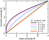Fig. 1. Kepler’s equation for five different eccentricities.

The innumerable publications about the solution of Kepler’s equation (Colwell 1993) highlight its importance in many fields of astrophysics (e.g. exoplanet search, planet formation, and star cluster evolution), astrodynamics, and trajectory optimisation. N-body hybrid algorithms also make use of this analytic solution of the two-body problem (Wisdom & Holman 1991). Nowadays, computers can solve Eq. (1) quickly. But the speed increase is counterbalanced by large data sets, simulations, and extensive data analysis (e.g. with Markov chain Monte Carlo). This explains ongoing efforts to accelerate the computation with software and hardware, for example by parallelising and use of graphic processing units (GPUs; Ford 2009).

The innumerable publications about the solution of Kepler’s equation (Colwell 1993) highlight its importance in many fields of astrophysics (e.g. exoplanet search, planet formation, and star cluster evolution), astrodynamics, and trajectory optimisation. N-body hybrid algorithms also make use of this analytic solution of the two-body problem (Wisdom & Holman 1991). Nowadays, computers can solve Eq. (1) quickly. But the speed increase is counterbalanced by large data sets, simulations, and extensive data analysis (e.g. with Markov chain Monte Carlo). This explains ongoing efforts to accelerate the computation with software and hardware, for example by parallelising and use of graphic processing units (GPUs; Ford 2009).

The Newton-Raphson iteration is a common method to solve Eq. (1) and employs the derivative E′. In each step n the solution is refined by

$$\begin{array}{c}\hfill E_{n+1}=E_n+E^{\prime }(M_n)(M-M_n)=E_n-\frac{E_n-esin{E}_n-M}{1-ecos{E}_n}·\end{array}$$(2)

A simple starting estimate might be E₀ = M + 0.85e (Danby 1987). Each iteration comes at the cost of evaluating one cosine and one sine function. Hence one tries to minimise the number of iterations. This can be done with a better starting estimate. For example, Markley (1995) provides a starting estimate better than 10⁻⁴ by inversion of a cubic polynomial which however requires also transcendental functions (four roots). Boyd (2007) further polynomialise Kepler’s equation through Chebyshev polynomial expansion of the sine term and yielded with root finding methods a maximum error of 10⁻¹⁰ after inversion of a fifteen-degree polynomial. Another possibility to reduce the iteration is to use higher order corrections. For instance Padé approximation of order [1/1] leads to Halley’s method.

Pre-computed tables can be an alternative way for fast computation of E. Fukushima (1997) used a table equally spaced in E to accelerate a discretised Newton method, while Feinstein & McLaughlin (2006) proposed an equal spacing in M, that is, a direct lookup table which must be e-dependent and therefore two-dimensional. Both tables can become very large depending on the desired accuracy.

So the solution of the transcendental Eq. (1) often comes back to other transcendental equations which themselves need to be solved in each iteration. This poses questions as to how those often built-in functions are solved and whether there is a way to apply a similar, more direct algorithm to Kepler’s equation.

The implementation details of those built-in functions are hardware and software dependent. But sine and cosine are often computed with Taylor expansion. After range reduction and folding into an interval around zero, Taylor expansion is here quite efficient yielding 10⁻¹⁶ with 17th degree at $\frac{\pi }{4}$. Kepler’s equation can also be Taylor expanded (Stumpff 1968) but that is less efficient, in particular for e = 1 and around M = 0 where the derivative becomes infinite. Similarly, root or arcsine functions are other examples where the convergence of the Taylor expansion is slow. For root-like functions, one again applies Newton-Raphson or bisection methods. The arcsine can be computed as $arcsin(x)=arctan(\frac{x}{\sqrt{1-x^2}})$ where Taylor expansion of the arctangent function is efficient and one root evaluation is needed.

An interesting alternative method to compute trigonometric functions is the Coordinate Rotation Digital Computer (CORDIC) algorithm which was developed by Volder (1959) for real-time computation of sine and cosine functions and which for instance found application in pocket calculators. CORDIC can compute those trigonometric and other elementary functions in a simple and efficient way. In this work we study whether and how the CORDIC algorithm can be applied to Kepler’s equation.

2. Scale-free CORDIC algorithm for Kepler’s equation

Analogous to CORDIC, we compose our angle of interest, E, by a number of positive or negative rotations σ_i = ±1 with angle α_i

$$\begin{array}{c}\hfill E_n={\displaystyle \sum _{i=1}^n{\sigma }_i{\alpha }_i.}\end{array}$$(3)

The next iteration n is then

$$\begin{array}{c}\hfill E_{n+1}=E_n+{\sigma }_{n+1}{\alpha }_{n+1}.\end{array}$$(4)

The rotation angle α_n is halved in each iteration

$$\begin{array}{c}\hfill {\alpha }_{n+1}=\frac{{\alpha }_n}{2}=\frac{{\alpha }_1}{2^n}\end{array}$$(5)

so that we successively approach E. The direction of the next rotation σ_{n + 1} is selected depending on the mean anomaly M_n calculated from E_n via Eq. (1). If M_n = E_n − e sin E_n overshoots the target value M, then E_{n + 1} will be decreased, otherwise increased

$$\begin{array}{c}\hfill {\sigma }_{n+1}=\{\begin{array}{cc}-1\hfill & E_n-esin{E}_n>M\hfill \\ +1\hfill & \text{else}.\hfill \end{array}\end{array}$$(6)

Equations (4)–(6) provide the iteration scheme which so far is a binary search or bisection method (with respect to E) to find the inverse of M (E). Choosing as start value E₀ = 0 and start rotation ${\alpha }_1=\frac{\pi }{2}$, we can cover the range E ∈ [ − π, π] and pre-compute the values of rotation angles with Eq. (5)

$$\begin{array}{cc}\hfill {\alpha }_n& =\frac{\pi }{2^n}·\hfill \end{array}$$(7)

The main difference of our algorithm from the CORDIC sine is the modified decision for the rotation direction in Eq. (6) consisting of the additional term e sin E. For the special case e = 0, the eccentric and mean anomalies unify and the iteration converges to E_n → E = M.

One major key point of CORDIC is that, besides the angle E_n, it propagates simultaneously the Cartesian representation, which are cosine and sine terms of E_n. The next iterations are obtained through trigonometric addition theorems

$$\begin{array}{cc}\hfill cos{E}_{n+1}& =cos(E_n+{\sigma }_{n+1}{\alpha }_{n+1})\hfill \end{array}$$(8)

$$\begin{array}{cc}& =cos{E}_{n}cos{\alpha }_{n+1}-{\sigma }_{n+1}sin{E}_{n}sin{\alpha }_{n+1}\hfill \end{array}$$(9)

$$\begin{array}{cc}\hfill sin{E}_{n+1}& =sin(E_n+{\sigma }_{n+1}{\alpha }_{n+1})\hfill \end{array}$$(10)

$$\begin{array}{cc}& ={\sigma }_{n+1}cos{E}_{n}sin{\alpha }_{n+1}+sin{E}_{n}cos{\alpha }_{n+1},\hfill \end{array}$$(11)

which is a multiplication with a rotation matrix

$$\begin{array}{c}\hfill \left(\begin{array}{c}{c}_{n+1}\\ s_{n+1}\end{array}\right)=\left[\begin{array}{cc}cos{\alpha }_{n+1}& -{\sigma }_{n+1}sin{\alpha }_{n+1}\\ {\sigma }_{n+1}sin{\alpha }_{n+1}& cos{\alpha }_{n+1}\end{array}\right]\left(\begin{array}{c}{c}_n\\ s_n\end{array}\right).\end{array}$$(12)

Here we introduced the abbreviations c_n = cos E_n and s_n = sin E_n.

Since the iteration starts with E₀ = 0, we simply have c₀ = cos E₀ = 1 and s₀ = sin E₀ = 0. The cos α_n and sin α_n terms can also be pre-computed using α_n from Eq. (7) and stored in a table listing the triples (α_n, cos α_n, sin α_n). Now we have eliminated all function calls for sine and cosine of E and α in the iteration. This is also true and important for the sin E_n term in Eq. (6) which is simply gathered during the iteration process as s_n via Eq. (12). Figures 2 and 3 illustrate the convergence for input M = 2 − sin2 ≈ 1.0907 and e = 1 towards E = 2.

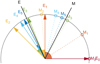Fig. 2. Example of five CORDIC rotations given M = 2 − sin2 ≈ 62.49° and e = 1. Starting with M0 = 0 and E0 = 0, Mn and En approach M and E = 2 ≈ 114.59°. The arcs indicates the current rotation angle αn and direction at each step.

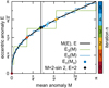Fig. 3. CORDIC-like approximation of Kepler’s equation (e = 1). The curves E3 and E5 illustrate the convergence towards Kepler’s equation after three and five iterations. The coloured points Mn, En are passed during the iterations to find E (M = 2 − sin2) (same colour-coding as in Fig. 2).

In Appendix A we provide a short python code which implements the algorithm described in this section. A slightly more elegant formulation is possible with complex numbers z_n = exp(iE_n) = cos E_n + i sin E_n and a_n = exp(iα_n)=cos α_n + i sin α_n. Then Eq. (12) becomes z_{n + 1} = a_{n + 1}z_n or $z_{n+1}=a_{n+1}^{\ast }{z}_n$ depending on σ_n and in Eq. (6) the substitution $sin{E}_n=\mathbb{I}m(z_n)$ has to be done.

A more detailed comparison with CORDIC is given Appendix B. Before analysing the performance in Sect. 5.3, we outline some optimisation possibilities in Sect. 3.

3. Variants and refinements

3.1. Minimal rotation base

The algorithms in Sect. 2 and Appendix B use always positive or negative rotation directions. While after n rotations the maximum error should be smaller then α_n, previous iterations can still be closer to the convergence limit. In Fig. 2, for instance, E₃ is closer to E than E₄ and E₅. Consecutive rotations will compensate this. A very extreme case is M = 0, where E₀ = 0 is already the exact value, but the first rotation brings it to E₁ = 90° followed by only negative rotation towards zero.

The CORDIC algorithm requires positive and negative rotations to have always the same scale K_n after n iterations (Appendix B). But since we could not pull out K_n from the iteration, we can depart from this concept and allow for only zero and positive rotations which could be called unidirectional (Jain et al. 2013) or one-sided (Maharatna et al. 2004). The decision to rotate or not to rotate becomes

$$\begin{array}{c}\hfill {\sigma }_{n+1}=\{\begin{array}{cc}1\hfill & (E_n+{\alpha }_{n+1})-esin(E_n+{\alpha }_{n+1})<M\hfill \\ 0\hfill & \text{else}.\hfill \end{array}\end{array}$$(13)

Thereby we compose E_n in Eq. (3) by minimal rotations and can expect also a better propagation of precision. Moreover, while the term sin(E_n + α_{n + 1}) = s_nc_a + c_ns_a still needs to be computed in each iteration to derive for σ_{n + 1}, the term c_{n + 1} is updated only when σ_{n + 1} = 1 which will be on average in about 50% of the cases. We note also that with the minimal rotation base the curve in Eq. (1) is approached from below.

3.2. CORDIC-like Newton method

The convergence of the CORDIC-like algorithms in Sects. 2 and 3.1 is linear, while Newton’s method is quadratic. Of course, our algorithm can serve start values (and their cosine and sine terms) for other root finders at any stage. The quadratic convergence should bring the accuracy from, for example, 10⁻⁸ down to 10⁻¹⁶ at the cost of mainly one division. We think this should be preferred over the other possible optimisations mentioned in Appendix B.

Still, we do not want to lose the ability to provide the cosine and sine terms after one (or more) Newton iterations. We can propagate them simultaneously in a similar manner as in Eqs. (4) and (12) but now using small angle approximations. Newton’s method Eq. (2) directly proposes a rotation angle

$$\begin{array}{c}\hfill {\alpha }_{n+1}=E_{n+1}-E_n=\frac{M-E_n+e{s}_n}{1-e{c}_n}·\end{array}$$(14)

This means that there is no need to check for a rotation direction σ_n. For small angles, there are the approximations sin α ≈ α and cos α ≈ 1. If one works with double precision (2⁻⁵³), the error $ϵ(\alpha )=|1-cos\alpha |<\frac{{\alpha }^2}{2}$ is negligible, meaning smaller than 2⁻⁵⁴ ≈ 5.5 × 10⁻¹⁷, when |α|< 7.5 × 10⁻⁹ (given for a₂₉). Then we can write

$$\begin{array}{cc}\hfill c_{n+1}& =c_n+{\alpha }_{n+1}{s}_n\hfill \end{array}$$(15)

$$\begin{array}{cc}\hfill s_{n+1}& =s_n+{\alpha }_{n+1}{c}_n.\hfill \end{array}$$(16)

3.3. Halley’s method

Halley’s method has a cubic convergence. Ignoring third order terms, one can apply the approximations sin α ≈ α and $cos\alpha \approx 1-\frac{{\alpha }^2}{2}$. The error $ϵ(\alpha )=|\alpha -sin\alpha |<|\frac{{\alpha }^3}{6}|$ is negligible in double precision, when $\alpha <\sqrt[3]{6\times 2^{-54}}=6.93\times {10}^{-6}$ given for α₁₉ ≈ 5.99 × 10⁻⁶. Similar to Sect. 3.2, the iteration scheme with co-rotation for Halley’s method is

$$\begin{array}{cc}\hfill {\alpha }_{n+1}& =\frac{(1-e{c}_n)(M-M_n)}{{(1-e{c}_n)}^2+\frac{1}{2}e{s}_n(M-M_n)}\hfill \end{array}$$(17)

$$\begin{array}{cc}\hfill s_{n+1}& =(1-\frac{{\alpha }_{n+1}^2}{2})s_n+{\alpha }_{n+1}{c}_n\hfill \end{array}$$(18)

$$\begin{array}{cc}\hfill c_{n+1}& =(1-\frac{{\alpha }_{n+1}^2}{2})c_n+{\alpha }_{n+1}{s}_n.\hfill \end{array}$$(19)

4. Hyperbolic mode

For eccentricities e ≥ 1, Kepler’s equation is

$$\begin{array}{c}\hfill M=esinhH-H.\end{array}$$(20)

This case can be treated as being similar to the elliptic case, when the trigonometric terms are replaced by hyperbolic analogues. Equations (6), (7), and (12) become

$$\begin{array}{cc}& {\sigma }_{n+1}=\{\begin{array}{cc}-1\hfill & esinh{H}_n-H_n>M\hfill \\ +1\hfill & \text{else}\hfill \end{array}\hfill \end{array}$$(21)

$$\begin{array}{cc}& {\alpha }_n=\frac{4ln2}{2^n}\hfill \end{array}$$(22)

$$\begin{array}{cc}& \left(\begin{array}{c}{c}_{n+1}\\ s_{n+1}\end{array}\right)=\left[\begin{array}{cc}cosh{\alpha }_{n+1}& {\sigma }_{n+1}sinh{\alpha }_{n+1}\\ {\sigma }_{n+1}sinh{\alpha }_{n+1}& cosh{\alpha }_{n+1}\end{array}\right]\left(\begin{array}{c}{c}_n\\ s_n\end{array}\right).\hfill \end{array}$$(23)

where a sign change in Eq. (23) leads to hyperbolic rotations. This equation set covers a range of H ∈ [ − 4 ln 2, 4 ln 2]. However, H extends to infinity. In the elliptic case, this is handled by an argument reduction which makes use of the periodicity. In the hyperbolic case, the corresponding nice base points H₀ are

$$\begin{array}{cc}& H_0=mln2\hfill \end{array}$$(24)

$$\begin{array}{cc}& c_0=cosh{H}_0=\frac{1}{2}[exp{H}_0+exp(-H_0)]=2^{m-1}+2^{-m-1}\hfill \end{array}$$(25)

$$\begin{array}{cc}& s_0=sinh{H}_0=\frac{1}{2}[exp{H}_0-exp(-H_0)]=2^{m-1}-2^{-m-1}.\hfill \end{array}$$(26)

For m = 0, this becomes H₀ = 0, c₀ = 1, and s₀ = 0, in other words similar to the elliptic case. For m ≠ 0, the start triple is still simple to compute using only additions and bitshifts.

The main challenge is to obtain the integer m from mean anomaly M. In elliptic case, this needs a division with 2π; in hyperbolic case, it becomes a logarithmic operation. Figure 4 and Appendix D show that

$$\begin{array}{c}\hfill m=\mathrm{sign}M·max[0,\mathrm{floor}(1+{log}_2\left|\frac{M}{e}\right|)]\end{array}$$(27)

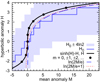Fig. 4. Range extension for hyperbolic Kepler’s equation (black curve) in case e = 1. The start value H0 (blue thick line) and the convergence domain of ±4 ln 2 (shaded area) covers Kepler’s equation. Nice base points (black dots) and two approximations (dotted and dashed curves) are also indicated.

provides start values with the required coarse accuracy of better than 4 ln 2. In floating point representation (IEEE 754), the second argument in the maximum function of Eq. (27) extracts simply the exponent of M/e. In fixed point representation, it is the most significant non-zero bit (Walther 1971). This means a logarithm call is not necessary (cf. Appendix A.2).

The hyperbolic iterations do not return cos H and sin H, but cosh H and sinh H which are the quantities needed to compute distance, velocity, and Cartesian position.

5. Accuracy and performance study

5.1. Accuracy of the minimal rotation base algorithm

The CORDIC-like algorithms have a linear convergence rate. The maximum error for E_n in iteration n is given by α_n. For instance, we expect from Eq. (7) α₂₂ < 10⁻⁶, α₂₉ < 10⁻⁸ (single precision), α₄₂ < 10⁻¹² and α₅₅ < 10⁻¹⁶ (double precision). To verify if double precision can be achieved in practice, we forward-calculated with Eq. (1) 1000 (M (E),E) pairs uniformly sampled in E over [0, π]. Here E might be seen as the true value. Then we injected M into our algorithms to solve the inverse problem E (M).

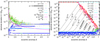
The differences between re-computed and true eccentric anomaly, δ₅₅ = |E₅₅ − E|, are shown in Fig. 5 for the cases e = 0.5, 0.9, and 1. For M ≳ 0.25 and e ≤ 1, the deviations are smaller than 10⁻¹⁵ and close to machine precision ϵ as indicated by the grey lines. Towards M = 0 and e > 0.9, the scatter increases. Figure 6 greatly magnifies this corner by plotting the deviations against the logarithm of E for e = 0.5, 0.999 999 999 9, and 1.

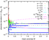Fig. 5. Accuracy. For visibility, zero deviations (δ = 0) within machine precision were lifted to δ = 2 × 10−17.

Fig. 6. Similar to Fig. 4, but with logarithmic scaling.

The deviations δ₅₅ become large in this corner, because the inversion of Eq. (1) is ill-posed. For e = 1, third order expansion of Eq. (1) is $M=E-(E-\frac{1}{6}{E}^3)=\frac{1}{6}{E}^3$. If the quadratic term in $1-\frac{1}{6}{E}^2$ is below machine precision ϵ, it cannot be propagated numerically in the subtraction and leads to a maximum deviation of $E<\sqrt{6ϵ}\approx {10}^{-8}$ at E = 10⁻⁸ (M = 10⁻²⁴).

Figure 7 illustrates the ill-posed problem. For e = 1 and very small M, the cubic approximation provides a very accurate reference. For comparison, we overplot our E₅₅ solution as well as computer generated pairs E-sin (E), E. Both exhibit a discretisation of 10⁻⁸ in E. We conclude that Newton’s, Halley’s, and other methods which directly try to solve Eq. (1) are as well only accurate to 10⁻⁸ in this corner when operating with double precision! Therefore, the M, E pairs mentioned above were not generated with built-in sin()-function but using a Taylor expansion of Kepler’s equations

$$\begin{array}{c}\hfill M=E(1-e)-e(-\frac{E^3}{3!}+\frac{E^5}{5!}-\cdots )·\end{array}$$(28)

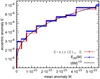Fig. 7. The ill-posed Kepler equation in the corner M = 0 and e = 1. Comparison of the computer approximations M (E) = E − e sin E (red) and our algorithm E55(M) (blue) with a cubic root (black; from well-posed inversion of a third-order Taylor expansion).

We may call the term in brackets rest function of sine. It differs by a factor of −E ⁻³ compared to its first naming in Stumpff (1959); see also Eq. (32).

We find that the deviations approximately follow the form

$$\begin{array}{c}\hfill {\delta }_{55}(E,e)=|E_{55}-E|\approx {10}^{-16}+{10}^{-16}\frac{E}{1-ecosE}+{10}^{-16}E,\end{array}$$(29)

as indicated by the curves in Figs. 5 and 6. For very small M and E, the constant term 10⁻¹⁶ dominates. Then the middle term, which is related to the derivative of Eq. (1), sets in. Finally, the linear term 10⁻¹⁶E takes over which describes the accuracy to which E can be stored. The middle term leads to an ascending and a descending branch which can be approximated by ${10}^{-16}\frac{E}{1-e}$ and ${10}^{-16}\frac{2}{E}$ and forms a local maximum. The two lines intersect at $E\approx \sqrt{2(1-e)}$ and ${\delta }_{55}(e)\approx {10}^{-16}\sqrt{\frac{2}{1-e}}$. For highest resolvable eccentricity below one, this provides $\delta (e=1-{10}^{-16})\approx \sqrt{2}\times {10}^{-8}$.

5.2. Accuracy of algorithm variants

We find that the algorithm with positive and negative rotations ($E_n^{+-}$, Sect. 2) provides slightly worse accuracy for all eccentricities (Fig. C.2). For instance for e = 0.9, it is limited to 10⁻¹⁵ and it ranges up to 10⁻⁵ for e = 1 at M = 10⁻¹⁶ (E = 10⁻⁵).

The combination of one final Newton iteration with E₂₉ as suggested in Sect. 3.2 has a similar accuracy as E₅₅ (in particular at e = 1) and provides therefore an alternative shortcut. The combination of one Halley iteration with E₁₉ has generally similar performance, but for high eccentricities it approaches 10⁻⁶.

5.3. Performance

Before we discuss some performance results, we should mention that a comparison of the algorithm speed is not simple. Depending on the hardware, multiplications might be little or much more expensive than additions. Then there is the question about the level of optimisation done in the code, by the compiler, or in built-in routines.

It can be also instructive to count the number of floating point operations. In Appendix A we see five multiplications, four additions, and one comparison in each iteration. For single precision this must be executed 29 times. On the other hand, a Newton iteration in Eq. (2) has one division, two multiplications, four additions, and one sine and cosine term. In case the latter two terms are computed via Taylor expansion to 17th order and with a Horner scheme, each will contribute additional nine multiplications and nine additions. Furthermore, the cosine and sine routines have to check the need for range reduction each time. Actually, also an additional final sine and cosine operation should be loaded to Newton’s methods, since sin E and cos E are usually needed in subsequent calculations.

Given same weight to all listed operations, we count approximately ten operations per CORDIC iteration vs. about per 43 operation per Newton iteration. Then we estimate that four CORDIC iteration are as expensive as one Newton iteration.

We have implemented both CORDIC-like and Newton’s method in a C program. The Newton’s method used the start guess E₀ = M + 0.85e and called cos and sin function from the standard math.h library. The run time was measured with python timeit feature for α₂₉ (10⁻⁸) and for 1000 mean anomalies uniformly sampled from 0 to π. The run-time of the CORDIC-like algorithm is independent of e, while Newton’s method is fast for small eccentricities and slower for high eccentricities. We measured that our CORDIC-like method has double, same, and half speed for e = 1, 0.01, and 0, respectively, or that 14 CORDIC-like iteration are as expensive as one Newton iteration.

5.4. Comparison with Fukushima (1997)

There are some similarities between this and the work of Fukushima (1997), and a comparison can be enlightening and useful to put our method in context. Fukushima (1997) uses a 128 long table sampled uniformly in E which provides an accuracy of 1/128. In contrast, we need a table of length log₂128 = 7 to obtain this accuracy and higher accuracy is not limited by a huge table. While Fukushima (1997) likely needs fewer iterations due to the use of discretised Newton method, we have no divisions.

Fukushima (1997) developed an iterative scheme with truncated Taylor series of Newton’s method to avoid recomputation of sine and cosine angles. Similar, our methods outlined in Sects. 3.2 and 3.3 avoids such recomputations by using truncated Taylor series for sine and cosine for small angles α_n. Our method appears less complex since it needs only three short equations.

5.5. Universal Kepler’s equation

Our algorithms can solve eccentric and hyperbolic Kepler’s equations. The two are very similar and could be unified, similar to the method in Walther (1971). Both algorithm includes also the eccentricity e = 1 (which are the limits for rectilinear ellipse and hyperbola, i.e. radial cases). The question is, therefore, whether our algorithm can also be applied to universal Kepler’s equation.

Following Fukushima (1999) and using the Stumpff function of third degree, c₃ (Stumpff 1959), the universal Kepler’s equation can be written as

$$\begin{array}{cc}\hfill L& =G+\kappa G^3{c}_3(\lambda G^2)\hfill \end{array}$$(30)

$$\begin{array}{cc}& =G+\kappa \frac{\sqrt{\lambda }G-sin\sqrt{\lambda }G}{{\sqrt{\lambda }}^3}\hfill \end{array}$$(31)

$$\begin{array}{cc}& =G+\kappa [\frac{G^3}{3!}-\frac{\lambda G^5}{5!}+\frac{{\lambda }^2{G}^7}{7!}-\cdots ]\hfill \end{array}$$(32)

with universal mean anomaly L, universal eccentric anomaly G, Brunnow’s parameter $\lambda =\frac{1-e}{1+e}$, and $\kappa =\frac{e}{1+e}$. In parabolic case (e = 1, λ = 0), it becomes a cubic equation. Using Eq. (31) and the relations $L=\frac{1+\lambda }{2{\sqrt{\lambda }}^3}M$ and $E=\sqrt{\lambda }G$, one can derive Kepler’s equation, Eq. (1) (see Appendix A in Fukushima 1999).

Equation (31) is expressed with a sine term. However, the application of a CORDIC-like algorithm to solve for G seems not possible due to the scaling term $\sqrt{\lambda }$ inside the sine function.

6. Summary

We show that the eccentric anomaly E from Kepler’s equation can be computed by a CORDIC-like approach and is an interesting alternative to other existing tools. The start vector E₀ = 0° and its Cartesian representation (cos E₀ = 1 and sin E₀ = 0) are rotated using a set of basis angles. The basis angles α_n and its trigonometric function values can be pre-computed and stored in an auxiliary table. Since the table is short and independent of e, it can be also hard-coded.

Our method provides E, sin E, and cos E without calling any transcendental function at run-time. The precision is adjustable via the number of iterations. For instance, single precision is obtained with n = 29 iterations. Using double precision arithmetic, we found the accuracy is limited to $\sim {10}^{-15}\sqrt{\frac{2}{1-e}}$ in the extreme corner (M = 0, e = 1). For accuracy and speed we recommend the one-sided algorithm described in Sect. 3.1.

Our method is very flexible. As a stand-alone method it can provide high accuracy, but it can be also serve start value for other refinement routines and coupled with Newton’s and Halley’s method. In this context we proposed in Sects. 3.2 and 3.3 to propagate cosine and sine terms simultaneously using small angle approximations in the trigonometric addition theorems and derived the limits when they can be applied without accuracy loss.

Though the number of iterations appears relatively large, the computational load per iteration is small. Indeed, a with simple software implementation we find a performance that is good competition for Newton’s method. However, CORDIC algorithms utilise their full potential when implemented in hardware, that is, directly as a digital circuit. So-called field programmable gate arrays (FGPA) might be a possibility to install our algorithm closer to machine layout. Indeed, hardware oriented approaches can be very successful. This was shown by the GRAvity PipelinE (GRAPE) project (Hut & Makino 1999), which tackled N-body problems. By implementing Newtonian pair-wise forces efficiently in hardware, it demonstrated a huge performance boost and solved new astrodynamical problems (Sugimoto et al. 2003).

Though we could not completely transfer the original CORDIC algorithm to Kepler’s equation, it might benefit from ongoing developments and improvement of CORDIC algorithms which is still an active field. In the light of CORDIC, solving Kepler’s equations appears almost as simple as computing a sine function.

Acknowledgments

The author thanks the referee Kleomenis Tsiganis for useful comments and M. Kürster and S. Reffert for manuscript reading. This work is supported by the Deutsche Forschungsgemeinschaft under DFG RE 1664/12-1 and Research Unit FOR2544 “Blue Planets around Red Stars”, project no. RE 1664/14-1.

References

Appendix A: Illustrative python code

The following codes implement the two-sided algorithms described in Sects. 2 and 4.

A.1. Elliptic case

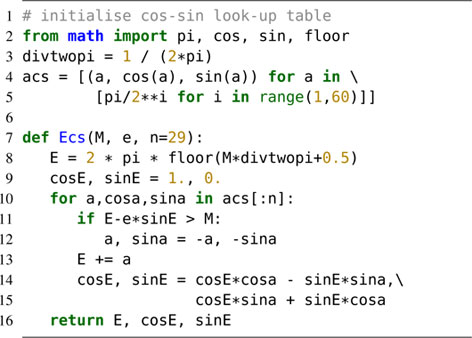
[linerange=9-15,33-41]kecordic.py

As an example, calling the function with Ecs(2-sin(2), 1) should return the triple (1.99999999538762, -0.4161468323531165, 0.9092974287451092).

We note that this pure python code illustrates the functionality and low complexity (not performance). An implementation in C (including a wrapper to python) and gnuplot with algorithm variants (e.g. one-sided for improved accuracy and speed) are available online¹.

A.2. Hyperbolic case

[linerange=44-50,70-81]kecordic.py

Calling Hcs(sinh(2)-2, 1) returns the triple (1.9999999991222275, 3.7621956879000753, 3.626860404544669).

The function frexp returns the mantissa and the exponent of a floating point number. Vice versa, the function ldexp needs a mantissa and an exponent to create a floating point number.

Appendix B: Comparison with original CORDIC algorithm for the sine

The CORDIC algorithm for the sine function is in practice further optimised to work solely with additive operation and bitshift operation and without multiplication or even division. The rotation angles α_n are slightly modified for this purpose such that now for n > 1

$$\begin{array}{c}\hfill tan{\alpha }_n=\frac{1}{2^{n-2}}·\end{array}$$(B.1)

As in Sect. 2, the first iteration starts with α₁ = 90° (tan α₁ = ∞). The second angle is also the same α₂ = 45° (tan α₂ = 1), while all other angles are somewhat larger than in Eq. (7) and the convergence range is $\sum _{n=1}^{\infty }{\alpha }_n=1.0549\pi =189.9°$. Using Eq. (B.1) we can write Eq. (12) as

$$\begin{array}{c}\hfill \left(\begin{array}{c}{c}_{n+1}\\ s_{n+1}\end{array}\right)=cos{\alpha }_{n+1}\left[\begin{array}{cc}1& -{\sigma }_{n+1}\frac{1}{2^{n-1}}\\ {\sigma }_{n+1}\frac{1}{2^{n-1}}& 1\end{array}\right]\left(\begin{array}{c}{c}_n\\ s_n\end{array}\right).\end{array}$$(B.2)

The next move in CORDIC is to take out the factor cos α_n from this equation and to accumulate it separately. This saves two multiplications, but changes the magnitude of the vector by cos α_n in each iteration and after n iteration by

$$\begin{array}{c}\hfill K_n={\displaystyle \prod _{i=2}^{n}cos{\alpha }_i=\prod _{i=2}^n\frac{1}{\sqrt{1+{tan}^2{\alpha }_i}}=\prod _{i=0}^{n-2}\frac{1}{\sqrt{1+4^{-i}}}·}\end{array}$$(B.3)

This scale correction factor K_n can be applied once after the last iteration. The iteration scheme for the scale dependent vector X_n, Y_n (where c_n = K_nX_n and s_n = K_nY_n) becomes

$$\begin{array}{cc}\hfill X_{n+1}& =X_n-Y_n\frac{{\sigma }_{n+1}}{2^{n-1}}\hfill \end{array}$$(B.4)

$$\begin{array}{cc}\hfill Y_{n+1}& =Y_n+X_n\frac{{\sigma }_{n+1}}{2^{n-1}}·\hfill \end{array}$$(B.5)

This could be applied for the solution of Eq. (1), too. However, the check for rotation direction in Eq. (6) requires then a scale correction (E_n − eK_nX_n > M). So one multiplication remains, while one multiplication can still be saved. The additional multiplication with e could be saved by including it into the start vector (i.e. z₀ = e exp(iE₀)=e = X₀ for E₀ = 0).

The final move in CORDIC is to map float values to integer values which has the great advantage that the division by a power of two can replaced by bit shifts. But since we could not eliminate all multiplications, the full concept of CORDIC is unfortunately not directly applicable to solve Kepler’s equation. Therefore, we call our method CORDIC-like.

However, it should be noted that also scale-free CORDIC algorithms have been developed (Hachaïchi & Lahbib 2016) at the expense of some additional bitshift operations. Furthermore, the scale correction K_n, which converges to K_∞ ≈ 0.607253 ≈ 1/1.64676, does not change in double precision for n = 26. This means from iteration n = 26 onwards, the concept of CORDIC is applicable, when setting the magnitude of the start vector to K₂₆e. Similar, for n = 29, the cosine term becomes one in double precision (cos α_n = 1), which also indicates a quasi-constant scale factor and means that we can save this multiplication. In Sects. 3.2 and 3.3 we exploit this fact in another way.

Appendix C: Accuracy plots

Fig. C.1. Similar to Figs. 5 and 6, but as function of E.

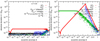Fig. C.2. Accuracy comparison of algorithm variants.

Appendix D: Starting estimate for the hyperbolic case

It can be shown that Eq. (27) always provides a lower bound for H in case of M ≥ 0. Starting with Kepler’s equation Eq. (20) and using the identity $sinhx=\frac{1}{2}[expx-exp(-x)]$ and the inequation exp(−x) ≥ 1 − 2x (for x ≥ 0), we obtain

$$\begin{array}{cc}\hfill M& =esinhH-H=\frac{e}{2}[expH-exp(-H)-2\frac{H}{e}]\hfill \\ \hfill & \le \frac{e}{2}[expH-1+2H(1-\frac{1}{e})]\hfill \\ \hfill & \le \frac{e}{2}[expH-1].\hfill \end{array}$$

For large values H, the approximation becomes more accurate. Further reforming and introduction of the binary logarithm yields

$$\begin{array}{cc}\hfill H& \ge ln(\frac{2M}{e}+1)=ln2·{log}_2(\frac{2M}{e}+1).\hfill \end{array}$$(D.1)

The right side of Eq. (D.1) is plotted in Fig. 4 as a red dotted line. It belongs to the family of start guesses given in Burkardt & Danby (1983) ($H_0=ln(\frac{2M}{e}+k)$). For $\frac{M}{e}=\frac{1}{2}$, e = 1, and H₀ = 0, the deviation is H − H₀ ≈ 1.396 = 2.014 ln 2. Since, unfortunately, the pre-factor is slightly larger than two, the convergence range is expanded to 4 ln 2 by setting α₁ = 2ln2 in Eq. (22).

For this large convergence range, we can further simply the start guess by omitting the additive one in Eq. (D.1)

$$\begin{array}{cc}\hfill H& >ln\frac{2M}{e}=ln2·{log}_2\frac{2M}{e}=ln2·(1+{log}_2\frac{M}{e})\hfill \end{array}$$(D.2)

$$\begin{array}{cc}& >ln2·\mathrm{floor}(1+{log}_2\frac{M}{e})\hfill \end{array}$$(D.3)

which finally leads to the start value for m in Eq. (27). The right function in Eq. (D.2) is plotted is in Fig. 4 as a blue dashed line. At $\frac{M}{e}=1$ and e = 1, the hyperbolic anomaly is H ≈ 1.729 = 2.495ln2 and thus inside our convergence domain.

The simple start guess developed here is valid for all e ≥ 1 and a lower bound for M ≥ 0, meaning that it is suitable for one-sided algorithms.

All Figures

	Fig. 1. Kepler’s equation for five different eccentricities.
In the text

	Fig. 2. Example of five CORDIC rotations given M = 2 − sin2 ≈ 62.49° and e = 1. Starting with M0 = 0 and E0 = 0, Mn and En approach M and E = 2 ≈ 114.59°. The arcs indicates the current rotation angle αn and direction at each step.
In the text

	Fig. 3. CORDIC-like approximation of Kepler’s equation (e = 1). The curves E3 and E5 illustrate the convergence towards Kepler’s equation after three and five iterations. The coloured points Mn, En are passed during the iterations to find E (M = 2 − sin2) (same colour-coding as in Fig. 2).
In the text

	Fig. 4. Range extension for hyperbolic Kepler’s equation (black curve) in case e = 1. The start value H0 (blue thick line) and the convergence domain of ±4 ln 2 (shaded area) covers Kepler’s equation. Nice base points (black dots) and two approximations (dotted and dashed curves) are also indicated.
In the text

	Fig. 5. Accuracy. For visibility, zero deviations (δ = 0) within machine precision were lifted to δ = 2 × 10−17.
In the text

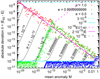	Fig. 6. Similar to Fig. 4, but with logarithmic scaling.
In the text

	Fig. 7. The ill-posed Kepler equation in the corner M = 0 and e = 1. Comparison of the computer approximations M (E) = E − e sin E (red) and our algorithm E55(M) (blue) with a cubic root (black; from well-posed inversion of a third-order Taylor expansion).
In the text

	Fig. C.1. Similar to Figs. 5 and 6, but as function of E.
In the text

	Fig. C.2. Accuracy comparison of algorithm variants.
In the text

References

- Boyd, J. P. 2007, Appl. Numer. Math., 57, 12 [CrossRef] [Google Scholar]
- Burkardt, T. M., & Danby, J. M. A. 1983, Celest. Mech., 31, 317 [NASA ADS] [CrossRef] [Google Scholar]
- Colwell, P. 1993, Solving Kepler’s Equation over three Centuries (Richmond, VA: Willmann-Bell) [Google Scholar]
- Danby, J. M. A. 1987, Celest. Mech., 40, 303 [NASA ADS] [CrossRef] [Google Scholar]
- Feinstein, S. A., & McLaughlin, C. A. 2006, Celest. Mech. Dyn. Astron., 96, 49 [NASA ADS] [CrossRef] [Google Scholar]
- Ford, E. B. 2009, New Ast., 14, 406 [NASA ADS] [CrossRef] [Google Scholar]
- Fukushima, T. 1997, Celest. Mech. Dyn. Astron., 66, 309 [NASA ADS] [CrossRef] [Google Scholar]
- Fukushima, T. 1999, Celest. Mech. Dyn. Astron., 75, 201 [NASA ADS] [CrossRef] [Google Scholar]
- Hachaïchi, Y., & Lahbib, Y. 2016, ArXiv e-prints [arXiv:1606.02468]. [Google Scholar]
- Hut, P., & Makino, J. 1999, Science, 283, 501 [NASA ADS] [CrossRef] [Google Scholar]
- Jain, A., Khare, K., & Aggarwal, S. 2013, Int. J. Comput. Appl., 63, 1 [Google Scholar]
- Maharatna, K., Troya, A., Banerjee, S., & Grass, E. 2004, IEE Proc. Comput. Digital Tech., 151, 448 [CrossRef] [Google Scholar]
- Markley, F. L. 1995, Celest. Mech. Dyn. Astron., 63, 101 [NASA ADS] [CrossRef] [Google Scholar]
- Stumpff, K. 1959, Himmelsmechanik (Berlin: VEB) [Google Scholar]
- Stumpff, K. 1968, Rep. NASA Tech. Note, 29, 4460 [Google Scholar]
- Sugimoto, D. 2003, in Astrophysical Supercomputing using Particle Simulations, eds. J. Makino, & P. Hut , IAU Symp., 208, 1 [NASA ADS] [Google Scholar]
- Volder, J. E. 1959, IRE Trans. Electron. Comput. 330 [CrossRef] [Google Scholar]
- Walther, J. S. 1971, in Proceedings of the May 18–20, 1971, Spring Joint Computer Conference (New York: ACM), AFIPS 71, 379 [Google Scholar]
- Wisdom, J., & Holman, M. 1991, AJ, 102, 1528 [NASA ADS] [CrossRef] [Google Scholar]