| Issue |
A&A
Volume 618, October 2018
|
|
|---|---|---|
| Article Number | A60 | |
| Number of page(s) | 8 | |
| Section | The Sun | |
| DOI | https://doi.org/10.1051/0004-6361/201833516 | |
| Published online | 12 October 2018 | |
Double plasma-resonance surfaces in flare loops and radio zebra emission
1
Astronomical Institute of the Czech Academy of Sciences, Fričova 298, 251 65 Ondřejov, Czech Republic
e-mail: This email address is being protected from spambots. You need JavaScript enabled to view it.
, This email address is being protected from spambots. You need JavaScript enabled to view it.
2
St.-Petersburg State University, 198504
St.-Petersburg, Russia
3
St.-Petersburg Branch of Special Astrophysical Observatory, 196140 St.-Petersburg, Russia
Received:
28
May
2018
Accepted:
11
July
2018
Abstract
Aims. The zebra structures observed in radio waves during solar flares are some of the most important structures used as diagnostics of solar flare plasmas. We here not only analyze the so-called double plasma-resonance (DPR) surfaces, but also estimate the effects of their form on the size of the zebra sources and brightness temperature.
Methods. To compute the DPR surfaces, we used numerical and analytical methods.
Results. We found that except for the case of a constant magnetic field across the loop, the DPR surfaces deviate from the constant plasma density surfaces. We found that the regime with a finite height scale has three forms of resonance surfaces depending on the magnetic field variation across the loop. This magnetic field variation also determines if in the generated zebra structure, an increase in gyro-harmonic number leads to an increase or decrease of the zebra stripe frequency. In the case with an infinite height scale, the resonance surfaces are parallel to the loop axis. Furthermore, we found that for highly polarized zebra structures that are generated at DPR surfaces close to the plasma frequency, the zebra emission is limited to the narrow escaping cone and the emitting source area increases with increasing viewing angle compared to the loop axis. Moreover, with increasing deviation of the DPR surfaces from those of constant density surfaces, the frequency bandwidth of the DPR emission increases and can cause the zebra stripes to overlap, which limits the zebra generation. For the zebra structures observed on 14 February 1999, 6 June 2000, and 1 August 2010 and the observed view perpendicular to the loop axis, we estimated that the brightness temperature is 3.67 × 10¹⁴ K, 6.58 × 10¹³ K, and 7.35 × 10¹⁵ K, respectively. These brightness temperatures are much lower than those derived for the view along the loop axis (up to 1017 K), and thus are more realistic. The area of the emitting source for coronal loops in the view perpendicular to the loop axis can be larger by several orders of magnitude than that in the view along the loop axis.
Key words: Sun: flares / Sun: radio radiation
© ESO 2018
1. Introduction
Zebra patterns (ZPs), appearing as regular stripes in emission and absorption in the dynamic spectra of solar radio bursts, are commonly known, and their observed characteristics and their models have been described in many papers (Slottje 1972; Kuijpers 1975; Zheleznyakov & Zlotnik 1975; Chernov 1976, 1990; LaBelle et al. 2003; Kuznetsov 2005; Bárta & Karlický 2006; Ledenev et al. 2006; Tan 2010; Karlický 2013; Zlotnik 2013; Tan et al. 2014; Chernov et al. 2018), see also the reviews by Chernov (2011, 2014). The most frequently discussed mechanism in the literature is that based on the double plasma-resonance (DPR) instability (Kuijpers 1975, 1980; Zheleznyakov & Zlotnik 1975; Mollwo 1983, 1988; Winglee & Dulk 1986; Yasnov & Karlický 2004; Kuznetsov & Tsap 2007; Chen et al. 2011; Karlický & Yasnov 2015; Yasnov et al. 2016, 2017; Benáček et al. 2017). In this model, owing to the DPR instability of superthermal electrons with the loss-cone type of distribution, the upper-hybrid waves are generated at the location in flare loops where the DPR condition is fulfilled. This condition is expressed as (1)
(1)
where fc, fup, and fp are the electron-cyclotron, upper-hybrid, and plasma frequencies, and s is the gyro-harmonic number. The upper-hybrid waves are then transformed into electromagnetic waves, which are then observed as radio zebra patterns. The layers in flare loops where the DPR condition is fulfilled are called the DPR resonance surfaces.
In all previous zebra models that were based on the DPR instability, the DPR surfaces are only arrayed along the loop axis without any specific form in the cross section of the loop, see the model of Zheleznyakov (1997), for instance. However, the DPR surfaces in flare loops are not only distributed along the loop axis, but have some form also across the loop because the plasma parameters change in the direction perpendicular to the loop axis. For zebra observations, the form of the DPR surface is important because the zebra emission, generated at frequencies close to that of the plasma frequency, can escape from its source only in a very narrow cone perpendicular to the DPR surface (Yasnov et al. 2017).
Yasnov et al. (2017) have recently shown that for a view of the zebra source along the zebra-source axis, where the plasma density varies in dependence on height and also along the source radius, the size of the emission region strongly depends on the density gradient along the source axis, that is, it depends on height when the zebra stripe sources are distributed vertically. For example, for the ratio of the height scale along the source axis and source half-width d in the range 1–3, the source size, which is given by the emission directivity, is only 0.006–0.018 d, see Fig. 2 in Yasnov et al. (2017). For the observed radio flux of zebras, this gives a very high brightness temperature of up to 1017 K, and it is not clear whether such a temperature is possible.
Therefore in this paper, we first analyze the form of the DPR surfaces across the loop and then present a new model of zebra sources where the DPR surfaces are observed from the direction perpendicular to the loop axis.
The paper is organized as follows: in Sect. 2 we analyze the DPR surfaces. In Sect. 3 we derive the sizes of the zebra source, estimate the brightness temperature for three observed zebras, and present the magnetic field structure of flaring loops with zebras. The conclusions are summarized in Sect. 4.
2. Analysis of the DPR surfaces in flare loops
It is known that the loop cross section along the loop axis in the corona is nearly constant, see Watko & Klimchuk (2000), for example. Thus, in the part of the loop where the zebra emission is generated, the magnetic field along its axis is assumed constant. Then only the magnetic field across the loop can be changed. The electron density and magnetic field in this part of the loop are (2)
(2)
and (3)
(3)
where n0 is the density at the loop axis at some reference level, r is the distance from the loop axis in the loop cross-section plane, d is the characteristic loop half-width, h is the height in the solar atmosphere, B0 is the magnetic field in the loop axis, y is the coordinate along the loop, and p h and pb are varying multiplication parameters. The term phd corresponds to the height scale H in the gravitationally stratified solar atmosphere.
We computed the DPR surfaces for several sets of parameters B0, n0, pb, ph. As an example, we selected the resonances with the gyro-harmonic numbers 26 and 27, which were determined for the zebra stripes at frequencies 1323 and 1301 MHz in the well-observed zebra pattern on 1 August 2010 (Yasnov et al. 2016). These frequencies and the corresponding resonances were also used for fitting, see below. Because the DPR surfaces have a symmetric form around the loop axis, we only present the cuts of these surfaces in the height-radius plane (the resonance lines) in the following.
2.1. Dependence of the DPR lines on the magnetic field parameter pb
As an example, we took a magnetic field of B0 = 17.2 G, a plasma density of n0 = 2 × 1011 cm−3, and a height scale of H = 3 d (ph = 3). We first considered the case with a constant magnetic field across the loop (pb = ∞). To determine the DPR lines, we used the same method as Karlický (2003). The DPR lines for the resonances (gyro-harmonic numbers) s = 26 (blue line) and s = 27 (red line) are shown in the left part of Fig. 1A. In the right part of this figure, the corresponding upper-hybrid (or after transformation, the radio) frequencies are added. The resonance lines follow the contours of the constant plasma densities, and the corresponding radio frequencies are constant across the loop.
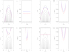 |
Fig. 1. DPR lines in the r/d–h/d plane (left parts of the panels) and the corresponding upper-hybrid (or radio) frequencies (right parts of the panels) for n0 = 2 × 1011 cm−3, B0 = 17.2 G and ph = 3. The red lines show the resonance s = 27 and blue lines show s = 26. In panels A, B, C and D, the magnetic parameter is pb = ∞, pb = 2, pb = 1 and |

Then we considered the cases with a varying magnetic field across the loop. We made computations with three values of the parameter pb = 2, 1, and  . The results for two resonances s = 26 (blue line) and s = 27 (red line) are shown in Figs. 1B–D, respectively. While in Fig. 1B the resonance lines are still oriented in the same direction as the plasma density contours, in Fig. 1C they are oriented in the opposite direction. Moreover, the red resonance line in Fig. 1B is inside the blue one, and in Fig. 1C, it is the opposite. A transition case, where the resonance lines are perpendicular to the loop axis, is shown in Fig. 1D. In all these cases, the intervals of the upper-hybrid (or radio) frequencies are very broad, see the right parts of these figures.
The parameters for the transition case (Fig. 1D) can be easily verified by analysis of Eq. (1). When we use relations for plasma and cyclotron frequencies in the form ![Mathematical equation: $ f_{\mathrm{p}} [\rm{MHz}] = 9 \times 10^{-3} \sqrt{n [\mathrm{cm}^{-3}]} $](/articles/aa/full_html/2018/10/aa33516-18/aa33516-18-eq6.gif) and fc[MHz]=2.8 × B [G], the resonance Eq. (1) can be expressed as
and fc[MHz]=2.8 × B [G], the resonance Eq. (1) can be expressed as (4)
(4)
Because the resonance lines in the transition case cannot be dependent on r, the parameter in the exponential function 2/pb2 needs to be equal to 1, which gives  . Then for the position of the resonance lines, we can write
 (5)
(5)
where fp0 and fc0 means the plasma and cyclotron frequency for the density n0 and the magnetic field B0. In our case with a plasma density n0 = 2 × 1011 cm−3, the magnetic field B0 = 17.2 G, and the parameter ph = 3, the values of  and h/d = 6.8 for s = 27 (red line) and h/d = 7.0 for s = 26 (blue line) agree with those in Fig. 1D.
If we increase the parameter pb, the resonant lines are closer to the plasma density contour and the frequencies in all resonances are closer to single frequencies. In the extreme case with pb = ∞, we have the case as presented in Fig. 1A.
2.2. DPR lines for H and ph ⇒∞
When we increase the height scale, in a broad range of this scale, a form of the resonance lines and the corresponding frequencies are similar to those presented in Fig. 1. This changes when the height scale H becomes infinite, however.
Using the same numerical method as in the previous paragraph, we computed the resonance lines for s = 26 (blue line) and 27 (red line) and for parameters B0 = 18.7 G, pb = 0.8, n0 = 2.2 × 1010 cm−3 and with the infinite ph (H = ∞), see Fig. 2A. In this case, the resonance lines are parallel and the corresponding frequencies are constant. In reality, this computation was made in order to fit the frequencies of two zebra stripes (1323 and 1301 MHz) of zebra structures on 1 August 2010 for the resonances s = 26 and 27 (Yasnov et al. 2016). In agreement with observations, the frequency corresponding to the resonance with s = 26 is greater than that for s = 27.
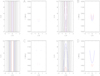 |
Fig. 2. DPR lines in the r/d–h/d plane (left parts of the panels) and the corresponding upper-hybrid (or radio) frequencies (right parts of the panels). The red lines and points show the resonance s = 27 and blue lines show s = 26. Panel A: for B0 = 18.7 G, pb = 0.8, n0 = 2.2 × 1010 cm−3 and with the infinite ph (height scale H = ∞). The right part of panel A is a fit of the frequencies for two zebra stripes (1323 MHz – s = 26 and 1301 MHz – s = 27 ) on 1 August 2010. Panel B: same as panel A, but for H = 100 d. Panel C: same as panel A, but for pb = 1.6 and n0 = 2.5 × 1010 cm−3. Panel D: same as panel C, but for H = 100 d. |
To see what happens when we decrease H to a lower value that still is very high, we computed the resonance lines for the same parameter as in the case shown in Fig. 2A, but with the height scale H = 100 d (ph = 100) (Fig. 2B). In this case, the resonance lines are not parallel, but diverge slightly for higher heights. The bandwidth of frequencies in the right part of Fig. 2B is given by the limited heights in the computational plane.
Both these cases (Figs. 2A and B) were made under the condition  . We now consider the cases with the opposite condition (
 ); we took pb = 1.6. We also slightly increased the density to n0 = 2.5 × 1010 cm−3 in order to have the resonances in the computational plane. The results are shown in Figs. 2C and D, where the infinite height scale and H = 100 d are considered. As in the case with H = ∞, the resonance lines are parallel and the frequencies are constant. In this case, however, the frequency of the resonance s = 26 is lower than that from the resonance with s = 27. When we decrease the height scale to H = 100 d, the resonance line converges for higher heights. Similarly as in the case presented in Fig. 2B, the bandwidth of frequencies in the right part of Fig. 2D is given by the limited heights in the computational plane.
The positions of the resonance lines in the cases where the height scale is close to infinity agree with those presented in Figs. 1B and C. As described above, the red resonance line in Fig. 1B is inside the blue one, and in Fig. 1C, it is opposite considering the relation between pb and  .
.
Thus, the condition  (or
(or  ) determines the zebras, where an increase in the resonance s is connected with a decrease in the zebra-stripe frequency (or with the increase in zebra-stripe frequency).
We verified the results with the infinite height scale analytically. Equation (2) in this case simplifies to (6)
(6)
Then the DPR condition can be written as (7)
(7)
where the solution for the resonance line position is (8)
(8)
where (9)
(9)
The solution in the regime  requires positive
  and in the regime
  negative
  . The positions of the zebra lines in Figs. 2A and C agree with those calculated from Eq. (8).
2.3. Emission bandwidth on the fundamental frequency for different directions to the observer
Radio zebras are usually highly polarized, which indicates that the emission frequency is close to the frequency of the upper-hybrid waves. This frequency is also close to the plasma frequency, however, which limits the emission into the cone with the angle (Zheleznyakov 1997) (10)
(10)
where ωL is the plasma frequency in the source and ω is the emission frequency. In conditions of the DPR, the ratio of these frequencies is (Karlický & Yasnov 2015) (11)
(11)
where s is the gyro-harmonic number. In the current case for s = 26 and 27, it is about Θmax = 2°.
To show how this emission cone limits the emitting frequencies, we analyzed the case we presented in Fig. 1B. The results are shown in Fig. 3, where we considered different directions to the observer (the direction perpendicular to the s = 27 resonance line at locations designated by the black point on this line (the central point of this emitting region expressed by the short black line). Figure 3A shows (emission along the loop axis) that the part of the resonance line that emits to the narrow cone (Θ max = 2°) is very small and the frequency bandwidth in this case is only 1 MHz. When the black point along the resonance line is shifted to greater distances from the loop axis, the part of the resonance line that emits to the escape cone increases and the frequency bandwidth of the emission also increases from 30 to 163 MHz (Figs. 3B–D).
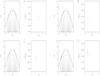 |
Fig. 3. DPR lines are the same as in Fig. 1 (panel B), but the frequencies from two resonance lines with s = 26 (blue) and 27 (red) (right parts of panels) are limited by the narrow emission cone (the half-width angle Θ max = 2°). The axis of this cone is oriented in the perpendicular direction to the s = 27 resonance line at the black point shown in the left part of panels A–D. The short black line on the s = 27 resonance line around the black point means the emitting part of the resonance line into the narrow escape cone. The emission frequency bandwidth from the s = 27 resonance line is 1 MHz, 30 MHz, 62 MHz and 163 MHz in panels A, B, C and D, respectively. |
If we interpret these bandwidths as those of zebra stripes, then this means that while in the case shown in Figs. 3A and B, where we can see distinct zebra stripes, in the case in Fig. 3D, the emission bandwidths from the neighboring zebra stripes for the resonances s = 26 and s = 27 overlap and thus no zebra can be observed. For the current loop parameters, the limiting case is that shown in Fig. 3C, where the emission bandwidth is 62 MHz. In this case, the angle between the loop axis and the direction to the observer is about 65°.
If we increase the parameter pb, then the resonant lines are closer to the plasma density contours and the emitting bandwidth becomes smaller in all parts of the resonance lines. Thus, the distinct zebra stripes can be observed for higher angles between the direction to the observer and the loop axis than in the previous case. In extreme cases with pb → ∞, the frequency bandwidth from all parts of the resonance line becomes zero.
The very narrow bandwidth of the emission from different resonance lines (needed for the zebra stripe observation) can also be found in the cases with the height scales close to infinity. For H = ∞, we obtain one single frequency from one resonance line. When the height scale is smaller but still very high, however, the bandwidth is limited mainly due to curvatures of the loop, which is expressed by the small and large loop radius, see below.
3. Zebra source sizes, brightness temperature, and magnetic field versus density structure of zebra-emitting flare loops
3.1. Radiation along the loop axis
As shown in the previous paragraph, in this case, the emitting resonance surface (limited by the narrow escaping cone) is very close to the constant density surface. Moreover, for high values of s considered here, the upper-hybrid frequencies are close to plasma frequencies. Then the extent of the emission region relative to d, for which the emission direction is nearly perpendicular to the constant-density profile, can be estimated as (Yasnov et al. 2017) (12)
(12)
where Θ max is the maximum escape angle of the plasma emission according to Eq. (10).
For example, for ph = 2 and Θmax ≈ 2°, the value of Δrsource/d = 0.0087.
Generally, the brightness temperature of the radio source can be expressed as (Zaitsev & Stepanov 1983) (13)
(13)
where F is the radio flux in SFU, fGHz is the frequency in GHz, and L8 (= 2Δrsource) is the dimension of the emission region in units of 108 cm.
Then, for example, for the zebra stripe (on 1323 MHz with s = 26) on 1 August 2010 (Yasnov et al. 2016), and for Θ max = 1.91°, radio flux F = 2900 SFU (measured by the Ondřejov radiospectrograph), and an assumed d = 1 Mm, the brightness temperature is equal to 8.48 × 10¹⁶ K, which is hardly possible. Moreover, as found in the previous section, in this case, only zebras can be generated where an increase of s gives an increase in zebra-stripe frequency.
Close to the loop axis, the resonance surfaces are always close to the constant density contours. However, for the parameter pb =  the emitting area equals the loop cross section, but in this case, the interval of emitting frequencies is very broad and thus the zebra stripes overlap.
3.2. Small changes in the magnetic field across the loop
The situation changes essentially when an emitting loop is observed from the direction perpendicular to the loop axis. Here we consider the case for pb → ∞, that is, the case where changes in magnetic field across the loop are very small and the resonant surfaces are nearly parallel to the constant density surfaces. This also means that the frequency bandwidth of the generated upper-hybrid waves is sufficiently narrow, and thus the zebra stripes do not overlap.
We estimated the source emitting area. We assumed that the density inside the loop can be expressed as in Eq. (2). Then for a location of the surface with the constant plasma density (the resonance surface in this case) we can write (see Eq. (6) in Yasnov et al. 2017) (14)
(14)
where C is some density constant. The derivation of this relation gives (15)
(15)
Then the angle between the loop axis and the line perpendicular to the constant density surface is (16)
(16)
Now, using Eq. (15), the length of the emitting region along the loop axis can be estimated with normalized variables rc = r/d and Hc = H/d = ph as (17)
(17)
The scales in the corona, where the zebras in the metric range are generated, are much larger than those in the chromosphere, where decimetric zebras are produced. While in the corona the height scale is in the interval of H = 50 ÷ 100 Mm (Gupta et al. 2015; Xie et al. 2017; H = 50 ÷ 100d for d = 1 Mm), in the chromosphere, H = 0.2 ÷ 1 Mm (H = 0.2 ÷ 1d for d = 1 Mm; Selhorst et al. 2008). Considering these height scales and taking Θmax = 2°, the area of the emitting region for coronal and chromospheric scales  , where (rcΘmax) is the size of the emitting region around the loop radius, is shown in Fig. 4. This area is much larger than the area of the region emitting along the loop axis. This essentially increases the probability of observing zebras from this emitting region.
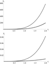 |
Fig. 4. Area of the emitting region Sc as a function of rc for d = 1 Mm. Top: for the coronal scales: H = 50 d (solid line) and H = 100 d (dashed line). Bottom: for the chromospheric scales: H = 0.2 d (solid line) and H = 1 d (dashed line). |
The difference of the areas for coronal and chromospheric scales explains the difference of zebra occurrence in the metric and decimetric ranges. Decimetric zebras are generated in low loops with high chromospheric densities, where the height scale is relatively small and thus the emitting region is small. As shown in Fig. 4, areas for coronal and chromospheric scales differ by several orders of magnitude.
In addition to these effects, the length of the emitting region along the loop axis can also be limited as a result of the loop curvature. To estimate this effect, we assumed that the loop has a semi-circular form with radius R. Then the length of the emitting region dhc is limited by the term ≈ R/d
Θ
max = Rc
Θ
max. Thus, the corrected length of the emitting region is (18)
(18)
The corresponding area of the emitting region is then (19)
(19)
Because the parameter  then only the zebras can be generated for which an increase of s gives an increase in zebra-stripe frequency.
When the parameter pb decreases, the magnetic field across the loop changes more rapidly and the resonance surfaces deviates more strongly from the constant density surfaces. Although the areas emitting in the direction perpendicular to the loop axis are also large, as in the case with pb → ∞, the problem is that with decreasing pb, the interval of the emitting frequencies increases and can exceed the separation frequency between neighboring zebra stripes and thus the zebra cannot be generated, see Fig. 3.
3.3. Case with H →∞
This case we expect at the part of the loop that is near the loop top. From a view in the direction perpendicular to the loop axis, the emitting area is large and the interval of emitting waves can also be sufficiently narrow for an observation of distinct zebra stripes, see Fig. 2. In this case, the emitting area is limited only by the curvatures of the loop, and it can be expressed as (20)
(20)
As shown in the previous paragraph, in this case, the two types of zebras can be generated where the increase of s is related to the increase or decrease of the zebra-stripe frequency.
Therefore we estimate the emitting area and brightness temperature of the zebras observed on 14 February 1999, 6 June 2000, and 1 August 2010, where the increase in s was found to be related with the decrease in zebra stripe frequency (Yasnov et al. 2016, 2017). Taking the zebra parameters from the literature (shown also in Table 1), we computed the brightness temperature for these three zebras, see Table 1. The brightness temperature is much lower than that derived by Yasnov et al. (2017), which is more realistic.
Zebra source parameters and zebra brightness temperature.
3.4. Magnetic field versus density structure of zebra-emitting flare loops
Karlický & Yasnov (2015) and Yasnov et al. (2016) described the relations between the magnetic field and plasma density for the zebra events from 14 February 1999, 6 June 2000, and 1 August 2010. They are shown here in Fig. 5. In agreement with the case presented in Sect. 3.3, these relations can be interpreted as those across the flaring loop. Figure 5 shows that an expected decrease in plasma density toward the loop edge is associated with a decrease in magnetic field.
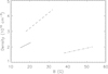 |
Fig. 5. Plasma density in dependence on the magnetic field across the loop for the zebras from 1 August 2010 (solid line), 14 February 1999 (dashed line), and 6 June 2000 (dash-dotted line). |
4. Conclusions
In agreement with the constant cross section of loops in the corona, we analyzed the DPR surfaces in the part of the flare loop where the magnetic field is constant along the loop axis and can change only in the direction perpendicular to its axis. In this part of the loop, the distribution of superthermal electrons that is unstable due to the DPR instability is assumed and thus generates the upper-hybrid waves at resonance surfaces and produces escaping electromagnetic waves (radio zebras) after their transformation.
We found that except for the case with the constant magnetic field across the loop, the DPR surfaces deviate from the constant plasma density surfaces. This deviation increases with decreasing parameter pb in Eq. (3). However, close to the loop axis, this deviation is always small.
We found that in the regime with a finite height scale H (the finite parameter ph), there are three forms of resonance surfaces in dependence on the relation between the parameter pb and  . While in the regime with
  , where the resonance surfaces are oriented in the same direction as the constant density surfaces, in the regime with
  , the resonance and constant density surfaces are oriented in the opposite direction. In the transition case with
  the resonance surfaces are perpendicular to the loop axis. In the case with the infinite height scale, the resonance surfaces are parallel to the loop axis.
Observations show zebras with high or low polarizations. The high polarization of zebras indicates that these zebras are generated close to the frequency of the upper-hybrid waves. For high values of the gyro-harmonic number we considered here, this frequency is close to the plasma frequency and thus the produced emission can escape only in a very narrow cone in the direction perpendicular to the resonance surface. This limits the zebra source area.
We found that owing to this limit, the emitting area in a view along the loop axis is always much smaller than that in a view in the direction perpendicular to the loop axis, except for the case with  , where the emitting area corresponds to the loop cross-section. Moreover, we found further limitations for the zebra stripe observations. Except for the case with a constant magnetic field across the loop, where the whole resonance surface emits in one single frequency, increasing the angle between the direction perpendicular to the resonance surface and loop axis, the frequency bandwidth of the emission increases due to the increase of deviations of DPR surfaces from constant density. Simultaneously, the emitting area increases. In our model case, we found that for an angle of about 65°, the frequency bandwidth of the zebra stripes equals the separation frequency between zebra stripes. This means that for higher viewing angles, the emission from different resonance surfaces overlaps, and thus zebras with distinct zebra stripes cannot be observed. However, for cases with height scales H → ∞, the zebra stripe bandwidth can be narrow and thus produce distinct zebra stripes. Another important characteristics of observed zebras is when an increase in resonance (gyro-harmonic) number s is related with the increase or decrease in zebra-stripe frequency.
In our model with the constant magnetic field along the loop axis, we found that for the emission from the region close to the loop axis, the zebra stripe frequency increases with the resonance number s. However, for the emission in the perpendicular direction, especially for the cases with H → ∞, the sequence of the zebra stripe frequency versus number s depends on the relation between the parameter pb and  . While in the case with
  the zebra stripe frequency increases with the increase of s, in the opposite case, the zebra stripe frequency increases with the decrease of s. We also showed that the emission from the DPR surfaces in the fundamental frequency (valid for the highly polarized zebras) is limited by the loop curvature.
For three observed zebras from 14 February 1999, 6 June 2000, and 1 August 2010, where the increase in s was related with the frequency stripe decrease, we estimated the brightness temperature as 3.67 × 10¹⁴ K, 6.58 × 10¹³ K, and 7.35 × 10¹⁵ K, respectively. We used the model with the infinite height scale and observing view perpendicular to the loop axis. These brightness temperatures are much lower than those derived for the view along the loop axis, and thus are more realistic. We also fit the frequencies of two zebra stripes on 1 August 2010.
In addition to all the limitations described above, the limits in the emission can be given by the spatial distribution of the DPR instability. This means that the upper-hybrid waves can be generated only in parts of DPR surfaces, and this limits the observed frequencies.
This spatial limit of the DPR instability is important especially for zebras generated on the second harmonic (low-polarized zebras), because the frequencies of the low-polarized zebras are well above the plasma frequency and therefore there is no limit due to the narrow escaping cone as for the highly polarized zebras.
Finally, if the magnetic field is changed along the part of the loop where the zebra is generated, for instance, in the loop footpoints, then the problem is more complex. We plan to analyze this in future work.
Acknowledgments
M. Karlický acknowledges support from Grants 16-13277S and 17-16447S of the Grant Agency of the Czech Republic. L.V. Yasnov acknowledges support from Grants 16-02-00254 and 18-02-00045 of the Russian Foundation for Basic Research, Program RAN #28, Project 1D and State Task No AAAA-A17-117011810013-4.
References
- Bárta, M., & Karlický, M.2006, A&A, 450, 359 [NASA ADS] [CrossRef] [EDP Sciences] [Google Scholar]
- Benáček, J., Karlický, M., & Yasnov, L. V.2017, A&A, 598, A106 [NASA ADS] [CrossRef] [EDP Sciences] [Google Scholar]
- Chen, B., Bastian, T. S., Gary, D. E., & Jing, J.2011, ApJ, 736, 64 [NASA ADS] [CrossRef] [Google Scholar]
- Chernov, G. P.1976, Sov. Astron., 20, 449 [Google Scholar]
- Chernov, G. P.1990, Sol. Phys., 130, 75 [NASA ADS] [CrossRef] [Google Scholar]
- Chernov, G.2011, Fine Structure of Solar Radio Bursts (Berlin: Springer) [Google Scholar]
- Chernov, G. P., Yan, Y.-H., & Fu, Q.-J.2014, Res. Astron. Astrophys., 14, 831 [NASA ADS] [CrossRef] [Google Scholar]
- Chernov, G. P., Fomichev, V. V., & Sych, R. A.2018, Geomag. Aeron., 58, 394 [CrossRef] [Google Scholar]
- Gupta, G. R., Tripathi, D., & Mason, H. E.2015, ApJ, 800, 140 [NASA ADS] [CrossRef] [Google Scholar]
- Karlický, M.2003, Sol. Phys., 212, 389 [NASA ADS] [CrossRef] [Google Scholar]
- Karlický, M.2013, A&A, 552, A90 [NASA ADS] [CrossRef] [EDP Sciences] [Google Scholar]
- Karlický, M., & Yasnov, L. V.2015, A&A, 581, A115 [NASA ADS] [CrossRef] [EDP Sciences] [Google Scholar]
- Kuijpers, J. M. E.1975, PhD Thesis, Utrecht, Rijksuniversiteit, The Netherlands [Google Scholar]
- Kuijpers, J.1980, in Radio Physics of the Sun, eds. M. R. Kundu, & T. E. Gergely, IAU Symp., 86, 341 [NASA ADS] [CrossRef] [Google Scholar]
- Kuznetsov, A. A.2005, A&A, 438, 341 [NASA ADS] [CrossRef] [EDP Sciences] [Google Scholar]
- Kuznetsov, A. A., & Tsap, Y. T.2007, Sol. Phys., 241, 127 [NASA ADS] [CrossRef] [Google Scholar]
- LaBelle, J., Treumann, R. A., Yoon, P. H., & Karlický, M.2003, ApJ, 593, 1195 [NASA ADS] [CrossRef] [Google Scholar]
- Ledenev, V. G., Yan, Y., & Fu, Q.2006, Sol. Phys., 233, 129 [NASA ADS] [CrossRef] [Google Scholar]
- Mollwo, L.1983, Sol. Phys., 83, 305 [NASA ADS] [CrossRef] [Google Scholar]
- Mollwo, L.1988, Sol. Phys., 116, 323 [NASA ADS] [Google Scholar]
- Selhorst, C. L., Silva-Válio, A., & Costa, J. E. R.2008, A&A, 488, 1079 [NASA ADS] [CrossRef] [EDP Sciences] [Google Scholar]
- Slottje, C.1972, Sol. Phys., 25, 210 [NASA ADS] [CrossRef] [Google Scholar]
- Tan, B.2010, Ap&SS, 325, 251 [Google Scholar]
- Tan, B., Tan, C., Zhang, Y., Mészárosová, H., & Karlický, M.2014, ApJ, 780, 129 [NASA ADS] [CrossRef] [Google Scholar]
- Watko, J. A., & Klimchuk, J. A.2000, Sol. Phys., 193, 77 [NASA ADS] [CrossRef] [Google Scholar]
- Winglee, R. M., & Dulk, G. A.1986, ApJ, 307, 808 [NASA ADS] [CrossRef] [Google Scholar]
- Xie, H., Madjarska, M. S., Li, B., et al. 2017, ApJ, 842, 38 [NASA ADS] [CrossRef] [EDP Sciences] [Google Scholar]
- Yasnov, L. V., & Karlický, M.2004, Sol. Phys., 219, 289 [NASA ADS] [CrossRef] [Google Scholar]
- Yasnov, L. V., Karlický, M., & Stupishin, A. G.2016, Sol. Phys., 291, 2037 [NASA ADS] [CrossRef] [Google Scholar]
- Yasnov, L. V., Benáček, J., & Karlický, M.2017, Sol. Phys., 292, 163 [NASA ADS] [CrossRef] [Google Scholar]
- Zaitsev, V. V., & Stepanov, A. V.1983, Sol. Phys., 88, 297 [NASA ADS] [CrossRef] [Google Scholar]
- Zheleznyakov, V. V.1997, Radiation in Astrophysical Plasmas [in Russian]; Original Russian Title – "Izlucheniye v astrofizicheskoy plasme" (Moscow: Yanus-K) [Google Scholar]
- Zheleznyakov, V. V., & Zlotnik, E. Y.1975, Sol. Phys., 44, 461 [NASA ADS] [CrossRef] [Google Scholar]
- Zlotnik, E. Y.2013, Sol. Phys., 284, 579 [NASA ADS] [CrossRef] [Google Scholar]
All Tables
All Figures
|
Fig. 1. DPR lines in the r/d–h/d plane (left parts of the panels) and the corresponding upper-hybrid (or radio) frequencies (right parts of the panels) for n0 = 2 × 1011 cm−3, B0 = 17.2 G and ph = 3. The red lines show the resonance s = 27 and blue lines show s = 26. In panels A, B, C and D, the magnetic parameter is pb = ∞, pb = 2, pb = 1 and |
| In the text | |
|
Fig. 2. DPR lines in the r/d–h/d plane (left parts of the panels) and the corresponding upper-hybrid (or radio) frequencies (right parts of the panels). The red lines and points show the resonance s = 27 and blue lines show s = 26. Panel A: for B0 = 18.7 G, pb = 0.8, n0 = 2.2 × 1010 cm−3 and with the infinite ph (height scale H = ∞). The right part of panel A is a fit of the frequencies for two zebra stripes (1323 MHz – s = 26 and 1301 MHz – s = 27 ) on 1 August 2010. Panel B: same as panel A, but for H = 100 d. Panel C: same as panel A, but for pb = 1.6 and n0 = 2.5 × 1010 cm−3. Panel D: same as panel C, but for H = 100 d. |
| In the text | |
|
Fig. 3. DPR lines are the same as in Fig. 1 (panel B), but the frequencies from two resonance lines with s = 26 (blue) and 27 (red) (right parts of panels) are limited by the narrow emission cone (the half-width angle Θ max = 2°). The axis of this cone is oriented in the perpendicular direction to the s = 27 resonance line at the black point shown in the left part of panels A–D. The short black line on the s = 27 resonance line around the black point means the emitting part of the resonance line into the narrow escape cone. The emission frequency bandwidth from the s = 27 resonance line is 1 MHz, 30 MHz, 62 MHz and 163 MHz in panels A, B, C and D, respectively. |
| In the text | |
|
Fig. 4. Area of the emitting region Sc as a function of rc for d = 1 Mm. Top: for the coronal scales: H = 50 d (solid line) and H = 100 d (dashed line). Bottom: for the chromospheric scales: H = 0.2 d (solid line) and H = 1 d (dashed line). |
| In the text | |
|
Fig. 5. Plasma density in dependence on the magnetic field across the loop for the zebras from 1 August 2010 (solid line), 14 February 1999 (dashed line), and 6 June 2000 (dash-dotted line). |
| In the text | |
Current usage metrics show cumulative count of Article Views (full-text article views including HTML views, PDF and ePub downloads, according to the available data) and Abstracts Views on Vision4Press platform.
Data correspond to usage on the plateform after 2015. The current usage metrics is available 48-96 hours after online publication and is updated daily on week days.
Initial download of the metrics may take a while.