| Issue |
A&A
Volume 618, October 2018
|
|
|---|---|---|
| Article Number | A41 | |
| Number of page(s) | 22 | |
| Section | Planets and planetary systems | |
| DOI | https://doi.org/10.1051/0004-6361/201833436 | |
| Published online | 11 October 2018 | |
Kepler Object of Interest Network★
II. Photodynamical modelling of Kepler-9 over 8 years of transit observations
1
Institut für Astrophysik,
Georg-August-Universität Göttingen,
Friedrich-Hund-Platz, 1,
37077 Göttingen, Germany
e-mail: This email address is being protected from spambots. You need JavaScript enabled to view it.
2
Stellar Astrophysics Centre, Aarhus University,
Ny Munkegade 120,
8000 Aarhus, Denmark
3
Rosseland Centre for Solar Physics, University of Oslo,
PO Box 1029 Blindern,
0315 Oslo,
Norway
4
Institute of Theoretical Astrophysics, University of Oslo,
PO Box 1029 Blindern,
0315 Oslo,
Norway
5
Astronomy Department, University of Washington,
Seattle,
WA 98195, USA
6
Institut d’Astrophysique de Paris,
98 bis Boulevard Arago,
75014 Paris,
France
7
Virtual Planetary Laboratory, University of Washington, USA
8
Leibniz-Institut für Astrophysik Potsdam,
An der Sternwarte 16,
14482 Potsdam,
Germany
9
Instituto de Astrofísica de Canarias,
C. Vía Láctea s/n,
38205 La Laguna,
Tenerife, Spain
10
Universidad de La Laguna,
Departamento de Astrofísica,
38206 La Laguna,
Tenerife, Spain
11
Aix-Marseille Université, CNRS, LAM, Laboratoire d’Astrophysique de Marseille, Marseille,
France
12
Department of Earth and Planetary Sciences, Weizmann Institute of Science,
Rehovot,
76100, Israel
13
School of Geosciences, Raymond and Beverly Sackler Faculty of Exact Sciences, Tel Aviv University,
Tel Aviv,
6997801, Israel
14
Institut de Cincies de l’Espai (IEEC-CSIC),
C. Can Magrans s/n, Campus UAB,
08193 Bellaterra, Spain
15
Institut Estudis Espacials de Catalunya (IEEC),
C. Gran Capit4,
Edif. Nexus,
08034 Barcelona, Spain
16
Hamburg Observatory, Hamburg University,
Gojenbergsweg 112,
21029 Hamburg,
Germany
17
Max Planck Institute for Astronomy,
Königstuhl 17,
69117 Heidelberg,
Germany
18
Instituto de Astronomía, UNAM, Campus Ensenada,
Carretera Tijuana-Ensenada km 103,
22860 Ensenada, México
Received:
16
May
2018
Accepted:
28
June
2018
Abstract
Context. The Kepler Object of Interest Network (KOINet) is a multi-site network of telescopes around the globe organised to follow up transiting planet-candidate Kepler objects of interest (KOIs) with large transit timing variations (TTVs). Its main goal is to complete their TTV curves, as the Kepler telescope no longer observes the original Kepler field.
Aims. Combining Kepler and new ground-based transit data we improve the modelling of these systems. To this end, we have developed a photodynamical model, and we demonstrate its performance using the Kepler-9 system as an example.
Methods. Our comprehensive analysis combines the numerical integration of the system’s dynamics over the time span of the observations along with the transit light curve model. This provides a coherent description of all observations simultaneously. This model is coupled with a Markov chain Monte Carlo algorithm, allowing for the exploration of the model parameter space.
Results. Applied to the Kepler-9 long cadence data, short cadence data, and 13 new transit observations collected by KOINet between the years 2014 and 2017, our modelling provides well constrained predictions for the next transits and the system’s parameters. We have determined the densities of the planets Kepler-9b and 9c to the very precise values of ρb = 0.439 ± 0.023 g cm−3 and ρc = 0.322 ± 0.017 g cm−3. Our analysis reveals that Kepler-9c will stop transiting in about 30 yr due to strong dynamical interactions between Kepler-9b and 9c, near 2:1 resonance, leading to a periodic change in inclination.
Conclusions. Over the next 30 years, the inclination of Kepler-9c (-9b) will decrease (increase) slowly. This should be measurable by a substantial decrease (increase) in the transit duration, in as soon as a few years’ time. Observations that contradict this prediction might indicate the presence of additional objects in this system. If this prediction turns out to be accurate, this behaviour opens up a unique chance to scan the different latitudes of a star: high latitudes with planet c and low latitudes with planet b.
Key words: planetary systems / planets and satellites: dynamical evolution and stability / methods: data analysis / techniques: photometric / stars: individual: Kepler-9 / stars: fundamental parameters
Ground-based photometry is only available at the CDS via anonymous ftp to cdsarc.u-strasbg.fr (130.79.128.5) or via http://cdsarc.u-strasbg.fr/viz-bin/qcat?J/A+A/618/A41
Guggenheim Fellow.
© ESO 2018
1 Introduction
One of the outstanding results of the Kepler mission (Borucki et al. 2010) is the large number of transiting multi-planet systems. Prior to Kepler’s launch, it was shown that the analysis of the dynamical interaction in multi-planet systems would be feasible offering an independent mass determination (Holman & Murray 2005; Agol et al. 2005). This was impressively confirmed from the first multi-transiting systems (Holman et al. 2010; Lissauer et al. 2011a) using transit timing variations (TTVs), that is, deviations from strict periodicity in planetary transits, caused by non-Keplerian forces. The first compilation of such systems revealed that multi-planet systems are preferentially found among lower-mass planets (Latham et al. 2011) highlighting the advantages of TTVs over radial velocity measurements. Since Kepler, the search for transiting multi-planetsystems has revealed objects such as TRAPPIST-1 (Gillon 2016), with three potentially habitable rocky planets, Kepler-80, a resonant chain of five planets, and Kepler-90, the first eight-planet system (Shallue & Vanderburg 2018).
Transiting multi-planet systems close to resonance allow for the determination of planetary radii and masses – and therefore bulk densities – from transit light curves alone, which has been intensively explored by Lissauer et al. (2011b), Jontof-Hutter et al. (2016), and Hadden & Lithwick (2017). A comparison between the two independent mass determinations, namely using radial velocity and transit timing variations, allows for the investigation of systematic errors due to observational and methodological biases (Mills & Mazeh 2017).
In order to tap into the dynamical information of TTVs it is important to cover a full cycle of orbital momentum and energy exchange between the planets (henceforth “interaction cycle”), which can be substantially longer than their orbital periods. One of the first lists of systems showing TTVs (Mazeh et al. 2013) revealed the large existing fraction of Kepler objects of interest (KOIs) that could not be used for dynamical analysis due to long interaction cycles. These were longer than, or of the order of, Kepler’s total observing time. This motivated us to create and coordinate the Kepler Object of Interest Network, (KOINet1, von Essen et al. 2018), a network of ground-based telescopes organised to follow up KOIs with large-amplitude TTVs. The main goal of KOINet is to coordinate already existing telescopes to characterise the masses of planets and planetary candidates by analysing their observed transit timing variations.
Among the KOINet targets, Kepler-9 is a benchmark system. The star is a solar analog and two of its planets are close to a 2:1 mean motion resonance, with TTV amplitudes of the order of one day. Their deep transits (~0.5 %) combined with their large interaction times and the magnitude of the host star (KP = 13.803) make this system ideal for photometric ground-based follow-up studies.
The first TTV analysis of the Kepler-9b/c system with an incomplete coverage of the interaction cycle had to be complemented with (a few) radial velocity measurements (Holman et al. 2010) which resulted in Saturn-mass planets. The composition of these two planets was investigated by Havel et al. (2011) from evolutionary models, as well as the stellar mass and radius. Using most or all long-cadence Kepler data, several authors revised the planetary masses from TTVs alone (Borsato et al. 2014; Dreizler & Ofir 2014) finding masses of about half the values previously reported in the first paper. Dreizler & Ofir (2014) thereby showed that the confirmed innermost planet, Kepler-9d, is dynamically independent from this near-resonant pair. Recently, a new transit observation for Kepler-9b (Wang et al. 2018b) was used to correct its transit time predictions. Additionally, the observation of the RossiterMcLaughlin effect in radial velocity measurements of Kepler-9 (Wang et al. 2018a) indicates that the stellar spin axis is very likely aligned with the planetary orbital plane.
In this paper, we exploit the large amount of short-cadence Kepler data, complemented by long-cadence Kepler data where short-cadence observations are missing, and extended three years in time by adding corresponding ground-based light curves from KOINet, all wrapped in a detailed photodynamical analysis. The observation of the full interaction cycle by the KOINet follow-up together with the comprehensive analysis results in Kepler-9b and 9c being the system with the highest-precision planetary mass and radius determinations. We also constrain the stellar parameters of the host star and predict the dynamical evolution of the system for the next few decades.
This paper is divided as follows. We describe the new transit observations by the KOINet, their reduction and analysis in Sect. 2. The structure of the photodynamical model used to analyse KOINet systems is described in Sect. 3. A description of the results from this analysis for the Kepler-9 system can be found in Sect. 4 and these results are discussed in Sect. 5. We end the paper with some conclusions in Sect. 6.
2 Observations, data reduction, and analysis
Between June, 2014, and September, 2017, we observed 13 primary transits of the Kepler-9b/c planets. The photometric follow-up was carried out in the framework of KOINet (von Essen et al. 2018). In this work, we combine the Kepler photometry with new ground-based data which have been collected after the nominal time of the Kepler Space Telescope. This section covers the treatment of the new ground-based observations. The photodynamical model described in Sect. 3 was previously fitted to the available Kepler data with the aim of obtaining initial parameters for the ground-based data analysis. A description of the photodynamical analysis on the different data sets follows in Sect. 4.
2.1 Data acquisition and main characteristics of the collected photometry
Table 1 shows the main characteristics of the data presented in this work. These are the date in which the observationswere performed, in years, months, and days; the planet observed during transit; an acronym for the telescope used to carry out the observations; the precision of the data in parts-per-thousand (ppt); the number of frames collected during the night, N; the cadence of the data accounting for readout time in seconds, CAD; the total duration of the observations in hours, Ttot; and the transit coverage, TC. To increase the photometric precision of the collected data, when possible we slightly defocused the telescopes (Kjeldsen & Frandsen 1992; Southworth et al. 2009).
Below is a brief description of the main characteristics of each of the telescopes involved in this work.
The Oskar Lühning Telescope (OLT 1.2 m) has a 1.2 m aperture diameter and is located at the Hamburger Observatory in Hamburg, Germany. The telescope can be used remotely and has a guiding system, minimising systematics caused by poor tracking. Although the seeing at the observatory is relatively poor (typical values are around 3–4 arcsec), it remains constant during the night, allowing photometric precision in the ppt level. Here we analyse one light curve taken during our first observing season.
The Apache Point Observatory hosts the Astrophysical Rese- arch Consortium 3.5 m telescope (henceforth “ARC 3.5 m”), and is located in New Mexico, in the United States of America. Due to the large collecting area, typically 2000 observations per observing run were collected with this telescope. For our observations, the telescope was slightly defocused. The photodynamical analysis of Kepler-9 presented here includes three light curves taken with the ARC 3.5 m during our second observing campaign in 2015.
The Wise Observatory hosts a 1 m telescope that is operated by Tel Aviv University, Israel (WISE 1 m). Here we present one transit taken during the second campaign in 2015.
The Centro Astronómico Hispano-Alemán hosts, among others, a 2.2 m telescope (henceforth “CAHA 2.2 m”). Here we present one complete transit observation of Kepler-9b.
The fully robotic 2 m Liverpool telescope (LIV 2 m; Steele et al. 2004) is located at the Observatorio Roque de los Muchachos and is owned and operated by Liverpool John Moores University. In this work, we present one transit observation taken with LIV 2 m during our second observing season.
The 2.5 m Nordic Optical Telescope (NOT 2.5 m) is located at the Observatorio Roque de los Muchachos in La Palma, Spain. Currently, telescope time for KOINet is assigned via a large (3 yr) program. Here, we analyse four light curves taken between the first and fourth observing seasons.
The 80 centimetre telescope of the Instituto de Astrofísica de Canarias (IAC 0.8 m) is located at the Observatorio del Teide, in the Canary Islands, Spain. Observations were collected by KOINet’s observers on site. Here we present one light curve taken during our second observing season.
The Telescopi Joan Oró (TJO) is a fully robotic 80 centimetre telescope located at the Observatori Astronomic del Montsec, in the north-east of Spain (henceforth “TJO 0.8 m”). Here we present one transit light curve.
The Observatorio Astronómico Nacional Llano del Hato, Venezuela, hosts a 1 m Zeiss reflector (henceforth “OANLH 1 m”). During scheduled observations, the telescope suffered from technical difficulties.
Characteristics of the collected ground-based transit light curves of Kepler-9b/c, collected in the framework of KOINet.
2.2 Data reduction and preparation
To reduce the impact of Earth’s atmosphere and the associated telluric contamination in the I-band, as well as the absorption of stellar light at shorter wavelengths, all of our observations are carried out using an R-band filter. Observers always provide a set of calibration frames (bias and flat fields) that are used to carry out the photometric data reduction. To reduce the data and construct the photometric light curves, we use our own IRAF and python-based pipelines called Differential Photometry Pipelines for Optimum light curves, DIP2 OL. A full description of DIP2OL can be found in von Essen et al. (2018). Briefly, the IRAF component of DIP2 OL measures fluxes for different reference stars, apertures, and sky rings; the latter two are set in proportion to the intra-night averaged full width at half maximum (FWHM). The python counterpart of DIP2 OL finds the optimum combination of reference stars, aperture, and width of the sky ring that minimises the scatter of the photometric light curves. Once the light curves are constructed, we transform the time stamps from Universal Time to Barycentric Julian Dates in Barycentric Dynamical Time (BJDTDB) using Eastman et al. (2010)’s web tool, all wrapped up in a python script.
To detrend the light curves, we compute the time-dependent x and y centroid positions of all the stars, the background counts from the sky rings, the integrated flat counts for the final aperture centered around the centroid positions, the airmass, and the seeing, all from the photometric science frames. A full description of our detrending strategy, how we combine these quantities to construct the detrending function, and the extra care in the particular choice and number of detrending parameters can be found in Sect. 4.2 of von Essen et al. (2018). The detrending components, and the time, flux, and errors, are injected into the transit fitting routine.
2.3 First data analysis
Before fitting the full data set using our photodynamical code (see Sect. 3) we carry out a transit fit to each ground-based light curve individually. The main goal of this step is to provide accurate error bars for the flux measurements, that are enlargedto account for correlated noise (see e.g. Carter & Winn 2009). A detailed description of the transit-fitting procedure can be found in Sect. 4 of von Essen et al. (2018). Briefly, once the detrending components are selected, we fit each transit light curve individually. For this, we use a detrending times transit (Mandel & Agol 2002) model, with a quadratic limb-darkening law and hence, quadratic limb-darkening coefficients. The latter are computed as described in von Essen et al. (2013), for stellar parameters closely matching the ones of Kepler-9 (Holman et al. 2010) and a Johnson–Cousins R filter transmission response. As initial values for all the transit parameters, we use the ones given by the photodynamical analysis carried out on Kepler data only. Since the TTVs in this system are so large, all of the transit parameters have to be computed for each specific light curve. When fitting for the transit parameters, rather than using uniform distributions for these parameters, we use Gaussian priors with mean and standard deviation equal to the values computed from our initial photodynamical analysis on Kepler data. Only when the transit is fully observed do we allow the model to fit for the semi-major axis, the inclination, and the planet-to-star radius ratio, along with the mid-transit time. Otherwise, all of the transit parameters remain fixed and we fit for the mid-transit time only.
To determine reliable errors for the fitted parameters, we compute them from posterior-probability distributions using a Markov chain Monte Carlo (MCMC) approach. At this stage, we iterate 100 000 times per transit, and discard a conservative first 20%. Once the best-fit parameters are obtained, we compute residual light curves by subtracting from the data our best-fit transit-times-detrending models. From the residuals we compute the β factor as fully described in Sect. 4.2 of von Essen et al. (2018). Here, we average β values computed in time bins of 0.8, 0.9, 1, 1.1, and 1.2 times the duration of ingress. If this averaged β factor is larger than 1, we enlarge the photometric error bars by this value, and we repeat the MCMC fitting in exactly the same fashion as previously explained. The raw light curves obtained after the second MCMC iteration with their error bars enlarged, along with the number of detrending components per light curve, are the input parameters of the photodynamical analysis. As a consistency check, after the photodynamical analysis is complete, we compare the derived detrending coefficients to the ones obtained from individually fitting the light curves.
2.4 Independent check of the timings
The use of KOINet to carry out TTV studies relates observations taken with several telescopes. As a consequence, the timings will be subject to the accuracy of the ground-based observatories, and the success of KOINet will rely on the capabilities of the many observatories involved in our photometric follow-up to accurately record timings.
In order to investigate this, on the night of July 25, 2015, we observed Kepler-9b using four different telescopes, namely CAHA 2.2 m, LIV 2 m, WISE 1 m, and NOT 2.5 m. Only in the case of CAHA 2.2 m did we have full transit coverage. After fitting for the transit parameters as previously specified, we obtained in this case the semi-major axis, a∕RS, the inclination, i, the planet-to-star radii ratio, RP ∕RS, and the mid-transit time, T0. The derived values along with their 1-σ uncertainties can be found in the top part of Table 2. Within errors, all the fitted parameters are consistent with the values predicted by our photodynamical analysis. The bottom part of the same table shows the individual mid-transit times obtained from fitting all the transit parameters for CAHA 2.2 m, and fixing all values except the mid-transit times for the remaining three. All mid-transit times are mutually consistent.
Figure 1 shows the quality of our reduction and analysis procedure. From top to bottom, we show the light curves of Kepler-9b obtained with CAHA 2.2 m in filled circles, LIV 2 m in empty squares, WISE 1 m in empty polygons, and NOT 2.5 m in filled diamonds. The light curves have been shifted to the predicted mid-transit time. Visual inspection confirms the equivalency of the derived mid-transit times. The consistency among mid-transit times alleviates the uncertainty that exists when using different sites to follow-up one target.
Transit parameters obtained fitting one light curve of Kepler-9b observed with CAHA 2.2 m on the night of 2015.07.25.
3 The photodynamical model
With the aim of producing a tool to determine planetary masses that is applicable to all of our KOINet objects, we developed a photodynamical model. Our light curve analysis is based on an n-body simulation of the planetary system over the time span of the observations, combined with a transit light curve model. The numerical integration is implemented in the Mercury6 package by Chambers (1999). We use the second-order mixed-variable symplectic (MVS) algorithm of the package, which is faster than the Bulirsch–Stoer (BS) algorithm but still applicable. The BS integrator would offer two advantages: the possibility of simulating close encounters and the precision in high-frequency terms of the Hamiltonian (discussed by Deck et al. 2014). The former is insignificant as the Kepler-9b/c system does not performclose encounters. The latter was tested to be negligible in our analysis. We calculated the difference of the same TTV model derived with the MVS integrator and the BS algorithm. Within a 50-yr integration, the difference shows a small slope, which can be corrected by a small change in the mean period smaller than 0.5 s and an oscillation with increasing amplitude. The amplitude of the oscillation is at most (in these 50 yr) of the order of 55 s which is of the order of the precision in the TTVs. For the 8 yr of Kepler-9 observations, the MVS integrator has sufficient precision. We added a first-order post-Newtonian correction (Kidder 1995) and wrote a python-wrapper for Mercury6 (Husser, priv. comm.). From the n-body simulation, we extract the projected distance between planets and star centres, that is in turn used to calculate the transit light curve through the Mandel & Agol (2002) model. Here we use a quadratic limb-darkening law already implemented in the occultquad routine. Finally, for each individual planets, we correct the output time by the light-travel-time effect.
As the numerical integration and its processing are computationally time consuming, we first carry out a coarse integration with a step size equal to only a twentieth of the period of the innermost simulated planet. A more detailed integration is produced for the parts where transits take place and where data are available. For these cases, the detailed integration is done with a step size of 0.01 days, which corresponds to a light curve accuracy of 0.01 ppm for long-cadence Kepler data. This accuracy is measured by the mean difference of transit light curves between a model with the given step size and a model with half the step size. For transit light curves, a time step comparable to ingress/egress duration would have a significant impact on the derivation of the transit parameters (Kipping 2010). Therefore, we calculate the transit model on a fine grid (~1 min, when needed) and we rebin this to the actual data points. We describe this in more detail in Sect. 4. For our model calculations, we define the x−y plane as the plane of the sky, with its origin placed at the stellar centre. Therefore, these coordinates coincide with the projected distances between planet and star mid points. The positive z-axis corresponds to the line of sight, so that the planets transit with positive z-values. The sampling of the Mercury6 integration does not match the observation times. To interpolate the projected distances from the Mercury6 results, we model them with a hyperbola in the range of a transit. The Mandel & Agol (2002) model is calculated for the observation points by these interpolated projected distances, quadratic limb darkening coefficients, and the planet-star radii ratios.
To explore the parameter space, our model is coupled to the MCMC emcee algorithm (Foreman-Mackey et al. 2013) accessible in the PyAstronomy2 library. All fitting parameters have uniform priors with large limits with the sole purpose of avoiding non-physical results. Our choice of free parameters is guided by the modelling rather than by the observations. For instance, Mercury6 uses the semi-major axis, a, of the planet as input value. Instead of the period, P, we therefore use a correction factor to a mean semi-major axis aadjust as a free parameter. The mean semi-major axis is calculated through Kepler’s third law from the mean period of the transit times of the planets. In addition, the mean anomaly, M, is calculated from this mean period, as well as the reference time, ΔT0. As a free parameter, we have an addend to this derived mean anomaly Madjust. Furthermore, Mercury6 uses the eccentricity, e, and the three angles that describe the position of the orbits on the sky. They are the orbital inclination, i, the argument of the periastron, ω, and the longitude of the ascending node, Ω. As the orientation in the plane of the sky is not directly measurable, Ω is fixed to zero for the innermost simulated planet. In this way, the corresponding values of the other planets show the difference in comparison to this first one. Last but not least, Mercury6 requires the masses, m, of the central star and the planets. These are given by an absolute value for the central star, the ratio of the masses of the innermost simulated planet to the central star, and the ratio of masses of the other planets to the innermost planet.
In order to calculate the transit light curve from the output of Mercury6, the stellar radius, RS, is required to calculate the relative planet-star distance normalised to the stellar radius. The transit measurements constrain the stellar density (Agol & Fabrycky 2017), but we choose to directly use the required model parameters. Instead of the stellar density, we input the stellar mass and radius, but fix one of them during the modelling. In addition, the occultquad routine requires the planet-star radius ratio, Rp ∕RS, and the two quadratic limb darkening coefficients, c1 and c2.
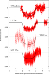 |
Fig. 1 Detrended transits of Kepler-9b observed on July 25, 2015, by four different telescopes. The transits are artificially shifted for better visual inspection, and plotted as a function of hours from the predicted mid-transit time to appreciate the duration of the observations. Each light curve has been labelled according to the corresponding telescope. |
4 Dynamical analysis of Kepler-9
Three different approaches were taken to dynamically characterise the Kepler-9b/c system. Firstly, in order to compare the photodynamical model with the dynamical analysis of only transit times, we fitted our model to quarters 1–16 of the Kepler long-cadence data (hereafter data set I). This allowed us to compare our results to those given by Dreizler & Ofir (2014). Secondly, we attempted to constrain the stellar radius by means of Kepler short-cadence data, since they have a sampling rate that is thirty times greater. To this end, we replaced Kepler long-cadence data with short-cadence data when available. Specifically, for Kepler-9, short cadence data are available between quarters 7 and 17 (data set II). Finally, the model is applied to the full data set, which comprises long-cadence data for Kepler quarters 1–6, short-cadence data covering quarters 7–17, and all new ground-based light curves, 13 in total, that were collected by KOINet (data set III).
The results from all the data analyses, and a comparison to previous analyses, are listed in Table 3. The top part of the table shows the stellar parameters. The literature values of the stellar radius and density parameters are taken from Havel et al. (2011), and the respective quadratic limb darkening values are taken from the NASA Exoplanet Archive (Mullally et al. 2015). The bottom part of Table 3 shows the derived planetary parameters. These are compared to the results given by Dreizler & Ofir (2014). In this latter work, the authors modelled the individual transits observed in long-cadence data, from where the mid-transit times were derived. Afterwards, they dynamically modelled these transit times.
The osculating orbital elements are given at a reference time, BJD = 2454933.0. Fitting the transit times found in Dreizler & Ofir (2014) with a linear time-dependent model we obtained the reference times Δ Tb = 25.26 d and Δ Tc = −3.08 d as intercepts, and the mean periods Pb = 19.247 d and Pc = 38.944 d as slopes. The reference times and mean periods are used for the determination of the semi major axis and the mean anomaly for all data sets, as described previously in Sect. 2.
During our photodynamical modelling we chose to fix the stellar mass to its literature value, mS = 1.05 ± 0.03 M⊙ (Havel et al. 2011). Derived parameters that depend on this value are the planetary masses, as the model parameters are given with respect to the stellar mass.Therefore, the uncertainties of the derived parameters are increased using error propagation including the uncertainty of the stellar mass,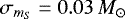 . When applied, in Table 3 these parameters are labelled with “
 prop.” The calculated densities of the star and the planets depend on the stellar mass in the same way. The semi-major axes are also affected. These are computed from the mean period through Kepler’s third law, which also includes the stellar and planetary masses. As a consequence, this error is also propagated into the uncertainty of the semi-major axis.
A quick comparative look at Table 3 shows how the limb darkening coefficients obtained modelling data set I significantly differ from their literature values. We address this issue in Sect. 5. With this exception, all planetary parameters are in agreement with prior results within 1-σ errors. The error bars decrease from modelling data set I to III. The reasons for this are given in detail in the following sections.
4.1 Treatment of the Kepler data
To prepare Kepler’s transit photometry we first extracted three times the transit duration symmetrically around each transit mid point. To account for intrinsic stellar photometric variability we normalised each transit light curve dividing this by a time-dependent second-order polynomial fitted to the out-of-transit data points. To obtain the coefficients of the polynomial functions, we used a simple least-squares minimisation routine. As previously mentioned, for long-cadence data, the light curve model is oversampled by a factor of 30 and rebinned to the actual data points. This procedure is not necessary for short-cadence data. The high signal-to-noise ratio (S/N) of Kepler data allowed us to include the quadratic limb darkening coefficients into our model budget.
4.2 Treatment of ground-based data
Due to the lower S/N of the ground-based data, we fixed the quadratic limb darkening coefficients to values derived from stellar evolution models for the R-band filter, which we used for all our observations. For stellar parameters closely matching the ones of Kepler-9, the derived limb darkening coefficients are c1 = 0.46 and c2 = 0.17. The best-matching coefficients of the previously derived detrending components (see Sect. 2.3) for each ground-based observation are calculated as a linear combination at each call of the photodynamical model.
4.3 Statistical considerations
We performed the analysis of data set I with 36 walkers each, iterating over 30 000 steps. The starting parameters of the walkers are randomly chosen from a normal distribution around the parameter results of Dreizler & Ofir (2014) with a 3-σ width. The walkers needed 2000 iterations to burn in, with the exception of one that finished in a higher χ2 minimum. Therefore, our results are derived from 35 walkers with 28 000 iterations each. We calculated the autocorrelation time for each parameter following Goodman & Weare (2010), but averaging over the autocorrelation function perwalker instead of averaging directly over the walker values, as discussed in the Blog by Daniel Foreman-Mackey3. These calculations result in an autocorrelation time of 1853 on average (2771 maximum), which gives us an effective sample size of 528 (353 minimum). Each parameter shows a Gaussian posterior distribution from which we extract the median and standard deviation values as best-fit values and errors, respectively. Our results are shown in Table 3. The best-fit solution has a reduced χ2 of 1.48.
The analysis of data set II is performed using 36 walkers with 20 000 iterations each. In this case, they burned in after 4000 iterations, with the exception of two walkers that ended in a higher χ2 minimum. The autocorrelation time averages out at 927 (1648 maximum), which gives an effective sample size of 586 (330 minimum). The resulting parameters are derived using the median and standard deviation of the posterior Gaussian distribution. The best solution of this analysis has a reduced χ2 of 1.06.
The modelling of data set III is accomplished by 36 walkers with 20 000 iterations each. Thirty-five of the walkers burned in after 2000 iterations. The resulting Gaussian distributions of the 630 000 iterations for the parameters and their correlations can be seen in Fig. A.7 for the mass-dependent parameters, in Fig. A.8 for the radius-dependent parameters, and in total in Fig. A.9. Our best-fit solution has a reduced χ2 of 0.97. The autocorrelation length of this analysis is given by a value of 694 on average (1105 maximum). This results in an effective sample size of 907 (570 minimum).
4.4 Results
The comparison of the best models to the most recent light curves from 2017 displayed in Fig. 2 clearly shows how the inclusion of our new ground-based light curves leads to an improvement of the derived parameters. The upper plot shows a Kepler-9b transit light curve in red observed on June 16, 2017. The lower plot shows a Kepler-9c transit light curve in blue observed on May 17, 2017. Both light curves were obtained using the NOT 2.5 m telescope. The variation of 500 randomly chosen good models for data set II is given by the light transparent yellow areas, which can be compared to the corresponding ones obtained including all new ground-based data (data set III). These are plotted in the figures with a light transparent black area. Additionally, the difference between the best model of each of the data sets II and III can be seen in the bottom panels of the plots (henceforth “residual plots”). Comparing the yellow and black areas shows a slight narrowing of the model variation for data set III, which is reflected by the slightly smaller error bars in Table 3. In the case of Kepler-9b, the transit models slightly shift towards earlier transits when all ground-based data are included. This can be seen by comparing the yellow and black areas, but it is more obvious in the residual plots. A larger change between modelling the different data sets appears for Kepler-9c. The residuals of the best model for this transit show an asymmetric difference between the modelling of data sets II and III. This means an adjustment not only in the transit time, but also in the transit shape.
The obtained detrended ground-based transit light curves are shown in Fig. A.1, together with the best photodynamical model in grey, and the variation of 500 randomly chosen good fitting models in black. The data corresponding to Kepler-9b are plotted in red, and the ones of Kepler-9c are plotted in blue. Each observation has its own sub-figure, where the date and the used telescope are indicated. The transits that were observed from different sites simultaneously are artificially shifted to allow for a visual inspection. Raw photometry is available for download.
Another derivable parameter of our photodynamical model is the transit times. Figure 3 shows the O-C diagram of the transit times measured by individually fitting the Kepler data, as well as the newly obtained ground-based data, in comparison to the results of modelling data set III. Also included is the mid-transit time of Kepler-9b obtained by Wang et al. (2018b), about 2σ off from our model and our new data. Unfortunately, the photometric data are not published so we could not include them in our photodynamic analysis. The top part of Fig. 3 shows the O-C diagram with the transit times from Kepler data in orange for Kepler-9b and in light blue for Kepler-9c. The O-C data from the new KOINet observations are shown in red for Kepler-9b and blue for Kepler-9c. The mid-time derived by Wang et al. (2018b) is shown in pink. The transit times from the best photodynamical model of data set III minus the linear trend are presented as grey lines. The middle part of this figure shows the residuals forKepler-9b with the same colour identification, and the residuals of Kepler-9c are shown respectively in the bottom part. In both residual plots, the 99.74% confidence interval of 1000 randomly chosen good models of the different data sets in comparison to the best model of data set III are plotted as grey areas. The light grey area belongs to the modelling of data set I, middle grey to data set II, and dark grey to data set III. The differences in the amplitude of the variations of the models compared to the best model are discussed in the following section. In Table A.1, we provide transit-time predictions from modelling data set III for the next 10 yr.
Stellar and planetary parameters derived from the photodynamical modelling of data set I in the second column, data set II in the third column, data set III in the fourth column, along with bibliographic values (Dreizler & Ofir 2014) in the fifth column for comparison and the sixth column displays some parameters corrected by investigating stellar evolution models in Sect. 5.4.
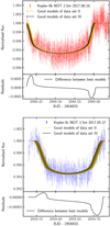 |
Fig. 2 Examples of newly obtained transit light curves for Kepler-9b in red (top), observed on June 16, 2017, and Kepler-9c in blue (bottom), observed on May 17, 2017. Both transits were observed using the NOT 2.5m telescope. Overplotted is the variation of 500 randomly chosen good models by modelling data set II (yellow) and data set III (black). The residuals plot shows the difference between the best models of these two data sets. |
5 Discussion
The results of the photodynamical modelling of Kepler-9b/c require some interpretation. In this section, we first discuss the dynamical stability of the derived system model, and subsequently we discuss the transit timing variations along with their prediction for future observations. We also specifically discuss the transit shape variations and the consequential prediction of disappearing transits for Kepler-9c. Moreover, we address the stellar activity and, connected to this, we investigate the stellar mass, radius, and age. The age is explored from stellar evolution models, as well as gyrochronologically. As the photodynamical modelling yields precise densities, our derived values are also the subject of discussion. Furthermore, the available radial velocity measurements of this system have not been mentioned in this paper; the reasons behind this choice are addressed below as well. The last point of this section deals with the innermost confirmed planet of the system, which is not included in the analysis. Finally, we discuss the possibility of detecting other planets in the system by means of the observed TTVs of Kepler-9b/c.
5.1 Dynamical stability
A dynamical analysis leads naturally to the question of the long-term stability of the derived planetary system, as an unstable result should not be considered as a viable model, contradicting the long lifetime of the system. To test the stability of our results for the Kepler-9 system, our best photodynamical solution was extended in time up to 1 Gyr. For this purpose, we used the second-order mixed-variable symplectic algorithm implemented in the Mercury6 package by Chambers (1999). This is the same integrator used in our photodynamical model. The post-Newtonian correction (Kidder 1995) has also been included for this application. The time step size we used was 0.9 days, which is slightly smaller than a twentieth of the period of the innermost planet considered in our dynamical analysis, Kepler-9b. This step size is a good compromise between reasonable computation time and small integration errors. We find that, over the integration time, the modelled planetary system remains stable. Given the architecture of the system, this was expected, and we can assume that the very similar good results from MCMC modelling should remain stable as well.
5.2 Transit timings
After the Kepler observations, as time progresses, good MCMC models differ from the best data set III model at varying amplitude (see for instance the time range around 2014–2015, and around 2018–2020; Fig. 3). These variations are illustrated by the grey areas in different shades for the modelling of the different data sets, from light to dark grey corresponding to data sets I, II, and III. At the specific times previously mentioned, the variations increase for both planets. This behaviour appears when the O-C has a positive slope for Kepler-9b, and a negative slope for Kepler-9c. At these places, the gradient of the TTVs is larger in comparison to the parts where Kepler-9b shows decreasing TTVs and when Kepler-9c shows increasing TTVs. A larger gradient leads to a larger uncertainty in the predictions. Despite the lower precision in comparison to the space-based Kepler data, the new ground-based KOINet observations help to set tighter constraints on the modulation of the timings. Unfortunately, apart from one observation, we missed the chance to observe transits in the phase of higher variation amplitude in 2014. The next period of higher-amplitude variation starts in 2018; a few more observations during 2018, especially of Kepler-9c transits, will help to further tighten constraints on this modulation.
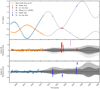 |
Fig. 3 O–C diagram of transit times from photodynamical modelling of data set III and the predictions until 2020 (top). Calculated (C) are transit times from a linear ephemeris modelled at the transit times found by Dreizler & Ofir (2014). The residual plots (middle: Kepler-9b; bottom: Kepler-9c) show the 99.74% confidence interval of 1000 randomly chosen good models in comparison with the best model of data set III. From light to dark grey: modelling of data set I, II, and III. The Kepler transit times are derived by single transit modelling. The new transit time data points originate from the first analysis described in Sect. 2.3. |
5.3 The disappearance of Kepler-9c transits
One of the advantages of our photodynamical modelling is the physical consistency in modelling variations in the transit shape due to variations in the transit parameters. These variations can be explained by the dynamical interaction of all objects in the system. Figure 4 shows these variations in the transit shape. Plotted are the transit light curve data per planet shifted by their individual transit time. For a better visualisation of this effect, we plotted only Kepler quarters 1–17 of the long-cadence data. The higher scatter of short-cadence data would lead to a larger range in flux. In turn, the variation of the model would appear diminished due to the larger data range. The model variation is shown in black, which is the best model for each of the transits modelled in data set III, shifted to a common time of transit. For Kepler-9c especially, a clear variation in the transit shape is visible, both in transit depth and transit duration.
The variation in transit shape is not only most visible from long-cadence data, but also most significant. The same TTV model with an averaged transit-shape model gives a 8% worse reduced χ2 on data set I. On data sets II and III, the difference in the reduced χ2 is only of the order of 0.5%. Nevertheless, photodynamical modelling has the advantage of consistently modelling the TTVs with the transit-shape-determining parameters, that is, mainly the inclination.
The observed variation in the transit shape of Kepler-9c leads us to examine the evolution of transit parameters over time. Figure 5 shows the variations of the semi-major axis, the eccentricity, and the inclination with the predictions for the next 50 yr. The predictions for the inclination of Kepler-9c show a continuous decrease, so that both the derived impact parameter b and the transit duration indicate the disappearance of the transits around the year 2052. This behaviour is shown in Fig. 5 as well. A long-term inspection reveals the variations in inclination to be a periodic effect, meaning that the transits will return around 2230 again (see Fig. A.2). Through the decreasing inclination, within the next 35 yr we will have the opportunity to map the high latitudes and hence measure the limb of Kepler-9 with frequent transit observations of planet c. In these higher latitudes, the transit spends more time atthe limb than in the case of a passage of the mid-point of the star. This fact could help us to obtain more information on the atmospheric structure at the limb.
On the other hand, for planet b, an increasing inclination in the next 100 yr is predicted (see Fig. A.2). Wang et al. (2018a) measured a stellar spin alignment with the planetary orbital plane on a high probability. As this result might be affected by stellar spot crossings, more RossiterMcLaughlin measurements are necessary for confirmation (Oshagh et al. 2016). Nevertheless, assuming spin alignment, Kepler-9b will scan the latitudes from its current location (above 30°), down to around 10°. With Kepler-9 being a solar analogue, a spot appearance similar to the sun between 0° and 30° is a reasonable assumption. Under those circumstances, we have a high probability of being able to measure spot crossings by Kepler-9b inprecise transit observations in the future. Such detections would lead to a starspot distribution measurement like in the work of Morris et al. (2017) in which the system analysed, HAT-P-11, is known to be highly misaligned. Therefore, an even more similar analysis is possible if the spin alignment of Kepler-9 is not confirmed, in which case there could possibly be spot contamination in the existing transit observations. Spot crossings are not resolvably measured inthese observations, meaning that a higher accuracy would be necessary for this analysis if they already occur.
The existing coverage of latitudes by transit observations is illustrated in Fig. A.3 under the assumption of a stellar spin alignment with the orbital plane. The red and blue lines refer to Kepler-9b and Kepler-9c transits, respectively. The track is extracted from the best photodynamical model of data set III. The uncertainties in these tracks are retrievable from the impact parameter shown in the fourth row of Fig. 5. The yellow circular disk illustrates the star and the orange area shows the possible star spot occurrence ranges assuming a similar behaviour to the sun.
The precise Kepler data allow us to model the quadratic limb darkening of the star. As a result, from modelling data set III, the derived limb darkening coefficients are c1 = 0.35 ± 0.05 and c2 = 0.27 ± 0.07. Figure A.8 shows that these two coefficients are highly anti-correlated. This result is consistent with Müller et al. (2013), who investigated the quadratic limb darkening of Kepler targets. Additionally, the values suit the literature values given in the NASA Exoplanet Archive (Mullally et al. 2015). The results from modelling data set I demonstrate that using only long-cadence Kepler data is not sufficient to model the quadratic limb darkening of Kepler-9. Nonetheless, the derived values of c1 = 0.28 ± 0.05 and c2 = 0.41 ± 0.09 fit the anti-correlation derived by modelling data set III. This anticorrelation is illustrated in the parameter correlation plot in Fig. A.8. Consequently, the discrepant values lead to different results for the stellar radius and the planet-star radius ratios.
In order to check for model-dependent influences on the resulting evolution of the system parameters, we investigated the differences between Newtonian gravity and the inclusion of a post-Newtonian correction. An analysis was done for the influence on resulting photodynamical models for Kepler-9b and c. Including the post-Newtonian correction decreased the parameter uncertainties in the second significant figure and the reduced χ2 in the fifth. The differences are too small to discriminate between the models. The future predictions for changes in inclination and for transit times behave very similarly.
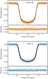 |
Fig. 4 All long-cadence Kepler (quarter 1−17) data perplanet, aligned by the transit time, in orange for Kepler-9b and in light blue for Kepler-9c. In grey is the best photodynamical model of the full data set, but calculated for only these Kepler long-cadence data and aligned respectively. The bottom of each figure shows the residuals. |
5.4 Stellar radius, mass, and age
Applying our photodynamical analysis to data set III, we determined a stellar density of ρS = 1.603 ± 0.061 g cm−3. As described in Sect. 3, we modelled the stellar radius instead of the density. However, the transit measurements constrain the stellar density (Agol & Fabrycky 2017). With a fixed stellar mass,the density can be determined straightforwardly. Our modelled density is almost 50% higher than the prior estimate ( ) by Havel et al. (2011). The authors derived this value from the TTV analysis of the first three quarters of Kepler observations by Holman et al. (2010). With this density, the stellar mass, radius, and age were determined by stellar evolution models. Our considerably higher derived density motivated a new, similar study of Kepler-9.
We used the stellar density and the known stellar parameters of an effective temperature Teff= 5777 ± 61 K, surface gravity logg = 4.49 ± 0.09 and metallicity Fe∕H = 0.12 ± 0.04 (which classifies Kepler-9 as a solar analogue; see Holman et al. 2010; Havel et al. 2011) to determine the age, mass, and radius of the star by stellar evolution models. The results are presented in the Appendix A (similar to Figs. 6 and 7 derived below) as a mass-age diagram in Fig. A.4 and as a radius-age diagram in Fig. A.5. We extracted the corresponding values from the interpolated MESA (Paxton et al. 2011, 2013, 2015) evolutionary tracks by MIST (Dotter 2016; Choi et al. 2016). We derive a stellar mass of 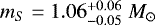 , a radius of
 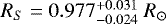 and an age of
 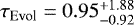 Gyr.
Gyr.
Recent HIRES observations by Petigura et al. (2017) of more than 1000 KOIs led to the correction of the Kepler-9 stellar parameters to Teff = 5787 ± 60 K, log g = 4.473 ± 0.1, and Fe ∕H = 0.082 ± 0.04. Although very similar, the lower metallicity leads to slightly different results. With these new values, we determined the stellar mass to  , the radius to
  and the stellar age to
  Gyr. The corresponding diagrams can be found for mass versus age in Fig. 6 and for radius versus age in Fig. 7. We note that mass and radius for both parameter sets are in agreement within 1σ. The derived age of 1.5 Gyr, however, is in better agreement with the gyrochronological age derived below. With these new values for the stellar mass and radius, we corrected the modelled planetary masses, semi-major axes, and radii, which can be found in the sixth column of Table 3.
More recently, the second Gaia data release (Gaia DR2) was carried out (Gaia Collaboration 2016, 2018). The effective temperature of  K derived using DR2 data fits the HIRES value within the 1σ range, as does the stellar radius with
  . These values have comparatively higher uncertainties, however. The distance of Kepler-9 is determined to p = 1.563 ± 0.017 mas by Gaia DR2.
To test the results of the stellar evolution model analysis, we determined the gyrochronological age of Kepler-9. For this, we computed a periodogram of Kepler-9’s full long-cadence photometry (Lomb 1976; Scargle 1982; Zechmeister & Kürster 2009). The highest power peak corresponds to 16.83 ± 0.08 days. The period and error correspond to the mean and standard deviation obtained fitting a Gaussian to the highest periodogram peak. On Kepler-9, typical photometric variability due to spot rotation has an amplitude of 5 ppt, well above the photometric noise.
To determine Kepler-9’s age we made use of Barnes (2007, 2009)’s gyrochronological estimate:
![Mathematical equation: \begin{equation*} \log(\tau_{\text{Gyro}}) = \frac{1}{n}[\log P - \log a - b \times \log (\text{B-V} - c)]\,, \end{equation*}](/articles/aa/full_html/2018/10/aa33436-18/aa33436-18-eq12.png) (1)
(1)
for a = 0.770 ± 0.014, b = 0.553 ± 0.052, c = 0.472 ± 0.027, and n =0.519 ± 0.007. Assuming B-V = 0.642, and following Barnes (2009) error estimates, the derived gyrochronological age for Kepler-9 is 2.51 ± 0.36 Gyr. This age is indicated in the mass-age and radius-age diagrams (Figs. 6, 7, A.4, and A.5) by green lines, solid for the the median value and dashed for the 1-σ range. The gyrochronological age is slightly higher than the age indicated by stellar evolution models, but the values agree within the 1-σ range.
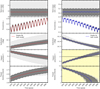 |
Fig. 5 Top: extrapolation of the planets semi-major axis until 2065 for the best model for Kepler-9b (red, left) and Kepler-9c (blue, right). Grey areas show the 99.74% confidence interval of 1000 randomly chosen good models for the different data sets. From light to dark grey: modelling of data sets I, II, and III. Second from top: extrapolation of the planets eccentricity. Third from top: extrapolation of the planets inclination. Fourth from top: extrapolation of the calculated impact parameter. Bottom: extrapolation of the calculated transit duration. The background of the impact parameter and the transit duration is coloured to highlight the place where the prediction of disappearing transits comes from. |
 |
Fig. 6 Mass-age diagram of Kepler-9 from MESA stellar evolution models (MIST). The black star and the red, orange, and grey dots correspond to the best-matching value and the 1, 2, and 3σ areas, respectively, derived from results on the density of the data set III photodynamical modelling and fromnew literature values of the effective temperature, the surface gravity, and the metallicity by Petigura et al. (2017). The gyrochronological age is indicated by the green solid line and its 1-σ range with the green dashed lines. |
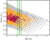 |
Fig. 7 Radius-age diagram of Kepler-9 from MESA stellar evolution models (MIST). The black star and the red, orange, and grey dots correspond to the best matching value and the 1, 2, and 3σ areas, respectively, derived from results on the density of the data set III photodynamical modeling and fromnew literature values of the effective temperature, the surface gravity, and the metallicity by Petigura et al. (2017). The gyrochronological age is indicated by the green solid line and its 1-σ range with the green dashed lines. |
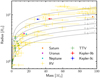 |
Fig. 8 Mass-radius diagram for known planets with masses up to 100 M⊕. In yellow are the planets with mass measurements obtained by radial velocities and in green the planets with mass measurements obtained from TTVs. The data are given by the The Extrasolar Planets Encyclopaedia. Our results are shown in red (Kepler-9b) and in blue (Kepler-9c). For comparison also the values of Saturn, Uranus, and Neptune are shown, the Neptune-like planet pair of our solar system. |
5.5 Stellar and planetary densities
In addition to the stellar density, the photodynamical analysis provides strong constraints on the planetary densities. As a result of the analysis performed on data set III, we obtain densities of ρb = 0.439 ± 0.023 g cm−3 for Kepler-9b and ρc = 0.322 ± 0.017 g cm−3 for Kepler-9c. In Fig. 8 our results are compared to literature values from The Extrasolar Planets Encyclopaedia4 for planets with similar properties. Colour-coded are the mass measurements obtained from radial velocities in yellow, and from TTVs in green. In this regime, that is the regime of Neptune-like planets, the density measurements of Kepler-9b/c are, to date, the most precise ones outside the solar system.
To rule out biased results for stellar radius and planet-star radii ratios caused by the photometric variability of Kepler-9, we checked for variability in the residuals of the transit light curves. For consistency, we chose the high-precision, well-sampled Kepler short-cadence data for this analysis. The scatter of the residuals inside the transit is slightly larger than outside the transit. For the best model of data set III, the standard deviation inside the transit is stdinside = 0.001049, while outside it is stdoutside = 0.001027, meaning a 2% difference between inside and outside the transit. We did not find any periodicity inside the transit residuals, potentially due to star spots. Equivalently, the transit time residuals do not show a periodic variability. Nevertheless, the higher scatter inside transit possibly results from unresolved stellar spot crossings. The planet-star radii ratio determination is affected within its uncertainties. With the absence of measurable star spots and the small differences in standard deviation between inside and outside the transit, a systematic error in the radius determination seems to be negligible. The planetary densities are therefore also well determined.
Figure 8 shows the similarity in radius of the Kepler-9b/c planets to Saturn. The masses are less than half the value of Saturn, resulting in smaller densities. Their low density implies Kepler-9b/c should be classified as hydrogen–helium gas giants. The formation of the planets happened most likely in the outer region of the system. Through converging migration, the planets could be brought in the near 2:1 mean motion resonance in close proximity to the host star (e.g. shown by Henrard 1982; Borderies & Goldreich 1984; Lemaitre 1984). It has been shown that such formation scenarios can result in stable resonant orbits with the outer planet having only about half the mass of the inner one (Deck & Batygin 2015).
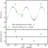 |
Fig. 9 Results from photodynamical modelling of data set III on the radial velocity measurements by Holman et al. (2010). |
5.6 Radial velocity measurements
In our analysis, we did not consider the radial velocity (RV) measurements by Holman et al. (2010) for Kepler-9. The reasons are the small number of measurements, the short time span of the observations, as well as the large discrepancy between a dynamical model to the TTVs and the RV data. Nevertheless, from our photodynamical model we calculated an RV model. Simulated RV models from the results of modelling the full transit dataset are shown together with the data in Fig. 9. The best model has a χ2 = 56.94 for the six RV measurements. As pointed out by Dreizler & Ofir (2014), we also see a similar discrepancy between the dynamical model and these measurements. Additional evidence in favour of the TTV model comes from the short-timescale chopping variations seen in planet 9b due to 9c: the amplitude of chopping indicates a smaller mass for planet 9c (Deck & Agol 2015), which, of course, is included in the full photodynamical constraint.
The most evident reason for this discrepancy is the activity of Kepler-9. A jitter factor would be necessary to include these data in the analysis. A detailed analysis of the activity of the star and the integration of the RV measurements is however, beyond the scope of this paper.
In addition, the recently obtained RV measurements listed in the HARPS-N archive5, but marked as proprietary, could help to better-constrain the RV behaviour of Kepler-9. Figure A.6 shows a prediction of the Kepler-9 radial velocity based on our model constraints for the approximate time span of the new HARPS-N observations.
5.7 An additional planet?
To completeour analysis, we also tested the influence of the third known planet, Kepler-9d (confirmed by Torres et al. 2011) with a period of Pd = 1.592960(2) d, on the dynamics of the system. We agree with Dreizler & Ofir (2014) that it does not interact measurably with the two modelled planets, in the plausible mass regime (md= 1–7 M⊕, Holman et al. 2010). For a mass of md = 7 M⊕, the reduced χ2 does not improve and also the variations of the residuals of the transit times are of the same order. The amplitude in radial velocity measurements is of the order of 1 m s−1, far below the precision of the previous observations and currently unfeasible for a star as faint as Kepler-9.
Adding another outer planet in a Laplace-resonance (4:2:1) to explain the deviations in the radial velocity measurements would require a rather high mass for the additional planet. Such a planet would have far too large an influence on the system’s dynamics and is ruled out by the photodynamical analysis. The fact that only six RV measurements are published makes it impossible to set constraints on further possible planets. Additional planets could exist outside the Laplace-resonance, thereby explaining the discrepancies between transit and radial velocity measurements, yet not substantially influencing the short-term dynamics. In addition we find no periodicity in the transit timing residuals, whereas evidence of periodicy here would have been a sign of an outer planet.
6 Conclusions
With this work, we substantiate the importance of the KOINet. With its anticorrelated, large-amplitude TTVs, the Kepler-9b/c system was chosen as a benchmark system for the photodynamical modelling. Although the dynamical cycle was almost covered by Kepler observations, the 13 new transit observations led to better constraints on the composition of the system. Concurrently, we have confirmed the capability of KOINet to complete a transit observation with a long duration by using several telescopes around the globe. This is complemented by the results of the photodynamical modelling. The application to Kepler-9 revealed that the transits of the outer planet will disappear in about 30 yr. Furthermore, this dynamical analysis of the combined photometric data, consisting of Kepler long- and short-cadence data in addition to ground-based follow-up observations led to the most precise planetary density measurements of planets in the Neptune-mass regime so far.
From the decreasing inclination of Kepler-9c and increasing inclination of Kepler-9b we have the opportunity to map the different latitudes of the star. Therefore, measurements of the limb and the star spots of Kepler-9 could be made possible by precise, frequent transit observations within the next 35 yr for the limb and 100 yr for the star spots. Interspersed with frequent ground-based follow-up, transit measurements from space that provide a high photometric precision would complement the stellar analysis. The promising predictions of this work make Kepler-9 an interesting target for space missions like TESS (Ricker et al. 2015), PLATO 2.0 (Rauer et al. 2014), or CHEOPS (Broeg et al. 2013), though it is a relatively faint object, with a Kepler magnitude of Kp = 13.803.
Acknowledgements
We acknowledge funding from the German Research Foundation (DFG) through grant DR 281/30-1. This work made use of PyAstronomy. CvE acknowledges funding for the Stellar Astrophysics Centre, provided by The Danish National Research Foundation (Grant DNRF106). Based on observations made with the Nordic Optical Telescope, operated by the Nordic Optical Telescope Scientific Association at the Observatorio del Roque de los Muchachos, La Palma, Spain, of the Instituto de Astrofísica de Canarias. We acknowledge support from the Research Council of Norways grant 188910 to finance service observing at the NOT. SW acknowledges support for International Team 265 (“Magnetic Activity of M-type Dwarf Stars and the Influence on Habitable Extra-solar Planets) funded by the International Space Science Institute (ISSI) in Bern, Switzerland. EA acknowledges support from United States National Science Foundation grant 1615315. EH and IR acknowledge support by the Spanish Ministry of Economy and Competitiveness (MINECO) and the Fondo Europeo de Desarrollo Regional (FEDER) through grant ESP2016-80435-C2-1-R, as well as the support of the Generalitat de Catalunya/CERCA programme. The Joan Oró Telescope (TJO) of the Montsec Astronomical Observatory (OAdM) is owned by the Generalitat de Catalunya and operated by the Institute for Space Studies of Catalonia (IEEC). Based on observations collected at the Centro Astronómico Hispano Alemán (CAHA) at Calar Alto, operated jointly by the Max-Planck Institut für Astronomie and the Instituto de Astrofísica de Andalucía (CSIC). Based on observations obtained with the Apache Point Observatory 3.5 m telescope, which is owned and operated by the Astrophysical Research Consortium. The Liverpool Telescope is operated on the island of La Palma by Liverpool John Moores University in the Spanish Observatorio del Roque de los Muchachos of the Instituto de Astrofisica de Canarias with financial support from the UK Science and Technology Facilities Council.
Appendix A Additional plots and a table of the transit time predictions
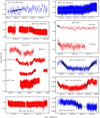 |
Fig. A.1 Our observed transits with the best model of data set III in grey and its variations by 500 randomly chosen good models in black. Transit data in red belong to Kepler-9b and blue transit data correspond to Kepler-9c. The transits from dates with more than one observation are artificially shifted for better visualisation and the telescope used is indicated. |
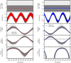 |
Fig. A.2 Top: extrapolation of the planets semi-major axis until 2550 for the best model in red (Kepler-9b) and blue (Kepler-9c) and in grey areas the 99.74% confidence interval of 1000 randomly chosen good models for the different data sets. From light to dark grey: modelling of data sets I, II, and III. Second from top: extrapolation of the planets’ eccentricity. Third from top: extrapolation of the planets inclination. Fourth from top: extrapolation of the calculated impact parameter. Bottom: extrapolation of the calculated transit duration. |
Ephemerides E and transit time predictions in BJD-2400000.0 from modelling data set III for the next 10 yr.
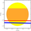 |
Fig. A.3 Latitude coverage of Kepler-9 (yellow circular disc) by all transit observations of data set III for Kepler-9b (red) and Kepler-9c (blue). Demonstrated is the best model of data set III. The order of the variations can be drawn from Figs. 5 or A.2, where the fourth row shows the modelled impact parameters. The orange area indicates the possible spot occurrence area between 0° and 30° up- and downwards. |
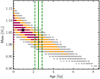 |
Fig. A.4 Mass-age diagram of Kepler-9 from MESA stellar evolution models (MIST). The black star and the red, orange, and grey dots correspond to the best matching value and the 1, 2, and 3σ areas, respectively, derived from results on the density of the data set III photodynamical modelling and from literature values of the effective temperature, the surface gravity, and the metallicity by Holman et al. (2010). The gyrochronological age is indicated by the green solid line and its 1-σ range with the green dashed lines. |
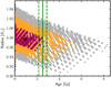 |
Fig. A.5 Radius-age diagram of Kepler-9 from MESA stellar evolution models (MIST). The black star and the red, orange, and grey dots correspond to the best matching value and the 1, 2, and 3σ areas, respectively, derived from results on the density of the data set III photodynamical modelling and from literature values of the effective temperature, the surface gravity, and the metallicity by Holman et al. (2010). The gyrochronological age is indicated by the green solid line and its 1-σ range with the green dashed lines. |
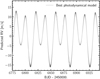 |
Fig. A.6 Predicted radial velocity measurements from the results of the photodynamical modelling of data set III for the approximate time span of the new observations listed in the HARPS-N archive |
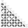 |
Fig. A.7 Correlation plot of masses, semi-major-axis, eccentricities, longitude of Periastron and mean anomaly from MCMC chains of modelling the full dataset. |
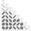 |
Fig. A.8 Correlation plot of stellar radius, inclination, planetary radii, argument of the ascending node of Kepler-9c and limb darkening coefficients from MCMC chains of modelling the full dataset. |
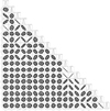 |
Fig. A.9 Full correlation plot of all fit parameters from modelling the full dataset. |
References
- Agol, E., & Fabrycky, D. 2017, in Handbook of Exoplanets, eds. H. J. Deeg & J. A. Belmonte (Springer Living Reference Work), 7 [Google Scholar]
- Agol, E., Steffen, J., Sari, R., & Clarkson, W. 2005, MNRAS, 359, 567 [NASA ADS] [CrossRef] [Google Scholar]
- Barnes, S. A. 2007, ApJ, 669, 1167 [NASA ADS] [CrossRef] [Google Scholar]
- Barnes, S. A. 2009, IAU Symp., 258, 345 [Google Scholar]
- Borderies, N., & Goldreich, P. 1984, Celest. Mech., 32, 127 [NASA ADS] [CrossRef] [MathSciNet] [Google Scholar]
- Borsato, L., Marzari, F., Nascimbeni, V., et al. 2014, A&A, 571, A38 [NASA ADS] [CrossRef] [EDP Sciences] [Google Scholar]
- Borucki, W. J., Koch, D., Basri, G., et al. 2010, Science, 327, 977 [NASA ADS] [CrossRef] [PubMed] [Google Scholar]
- Broeg, C., Fortier, A., Ehrenreich, D., et al. 2013, Eur. Phys. J. Web Conf., 47, 03005 [CrossRef] [EDP Sciences] [Google Scholar]
- Carter, J. A., & Winn, J. N. 2009, ApJ, 704, 51 [NASA ADS] [CrossRef] [Google Scholar]
- Chambers, J. E. 1999, MNRAS, 304, 793 [NASA ADS] [CrossRef] [MathSciNet] [Google Scholar]
- Choi, J., Dotter, A., Conroy, C., et al. 2016, ApJ, 823, 102 [NASA ADS] [CrossRef] [Google Scholar]
- Deck, K. M., & Agol, E. 2015, ApJ, 802, 116 [NASA ADS] [CrossRef] [Google Scholar]
- Deck, K. M., & Batygin, K. 2015, ApJ, 810, 119 [Google Scholar]
- Deck, K. M., Agol, E., Holman, M. J., & Nesvorný, D. 2014, ApJ, 787, 132 [CrossRef] [Google Scholar]
- Dotter, A. 2016, ApJS, 222, 8 [NASA ADS] [CrossRef] [Google Scholar]
- Dreizler, S., & Ofir, A. 2014, ArXiv e-prints [arXiv:1403.1372] [Google Scholar]
- Eastman, J., Siverd, R., & Gaudi, B. S. 2010, PASP, 122, 935 [NASA ADS] [CrossRef] [Google Scholar]
- Foreman-Mackey, D., Hogg, D. W., Lang, D., & Goodman, J. 2013, PASP, 125, 306 [CrossRef] [Google Scholar]
- Gaia Collaboration ( Prusti, T., et al.) 2016, A&A, 595, A1 [NASA ADS] [CrossRef] [EDP Sciences] [Google Scholar]
- Gaia Collaboration (Brown, A. G. A., et al.) 2018, A&A, 616, A1 [NASA ADS] [CrossRef] [EDP Sciences] [Google Scholar]
- Gillon, M., Jehin, E., Lederer, S. M., et al. 2016, Nature, 533, 221 [NASA ADS] [CrossRef] [PubMed] [Google Scholar]
- Goodman, J., & Weare, J. 2010, Commun. Appl. Math. Comput. Sci., 5, 65 [Google Scholar]
- Hadden, S., & Lithwick, Y. 2017, AJ, 154, 5 [NASA ADS] [CrossRef] [Google Scholar]
- Havel, M., Guillot, T., Valencia, D., & Crida, A. 2011, A&A, 531, A3 [NASA ADS] [CrossRef] [EDP Sciences] [Google Scholar]
- Henrard, J. 1982, Celest. Mech., 27, 3 [NASA ADS] [CrossRef] [MathSciNet] [Google Scholar]
- Holman, M. J., & Murray, N. W. 2005, Science, 307, 1288 [NASA ADS] [CrossRef] [PubMed] [Google Scholar]
- Holman, M. J., Fabrycky, D. C., Ragozzine, D., et al. 2010, Science, 330, 51 [NASA ADS] [CrossRef] [PubMed] [Google Scholar]
- Jontof-Hutter,D., Ford, E. B., Rowe, J. F., et al. 2016, ApJ, 820, 39 [NASA ADS] [CrossRef] [Google Scholar]
- Kidder, L. E. 1995, Phys. Rev. D, 52, 821 [NASA ADS] [CrossRef] [Google Scholar]
- Kipping, D. M. 2010, MNRAS, 408, 1758 [NASA ADS] [CrossRef] [Google Scholar]
- Kjeldsen, H., & Frandsen, S. 1992, PASP, 104, 413 [NASA ADS] [CrossRef] [Google Scholar]
- Latham, D. W., Rowe, J. F., Quinn, S. N., et al. 2011, ApJ, 732, L24 [NASA ADS] [CrossRef] [Google Scholar]
- Lemaitre, A. 1984, Celest. Mech., 34, 329 [NASA ADS] [CrossRef] [Google Scholar]
- Lissauer, J. J., Fabrycky, D. C., Ford, E. B., et al. 2011a, Nature, 470, 53 [NASA ADS] [CrossRef] [PubMed] [Google Scholar]
- Lissauer, J. J., Ragozzine, D., Fabrycky, D. C., et al. 2011b, ApJS, 197, 8 [NASA ADS] [CrossRef] [Google Scholar]
- Lomb, N. R. 1976, Ap&SS, 39, 447 [NASA ADS] [CrossRef] [Google Scholar]
- Mandel, K., & Agol, E. 2002, ApJ, 580, L171 [NASA ADS] [CrossRef] [Google Scholar]
- Mazeh, T., Nachmani, G., Holczer, T., et al. 2013, ApJS, 208, 16 [NASA ADS] [CrossRef] [Google Scholar]
- Mills, S. M., & Mazeh, T. 2017, ApJ, 839, L8 [NASA ADS] [CrossRef] [Google Scholar]
- Morris, B. M., Hebb, L., Davenport, J. R. A., Rohn, G., & Hawley, S. L. 2017, ApJ, 846, 99 [NASA ADS] [CrossRef] [Google Scholar]
- Mullally, F., Coughlin, J. L., Thompson, S. E., et al. 2015, ApJS, 217, 31 [Google Scholar]
- Müller, H. M., Huber, K. F., Czesla, S., Wolter, U., & Schmitt, J. H. M. M. 2013, A&A, 560, A112 [NASA ADS] [CrossRef] [EDP Sciences] [Google Scholar]
- Oshagh, M., Dreizler, S., Santos, N. C., Figueira, P., & Reiners, A. 2016, A&A, 593, A25 [NASA ADS] [CrossRef] [EDP Sciences] [Google Scholar]
- Paxton, B., Bildsten, L., Dotter, A., et al. 2011, ApJS, 192, 3 [Google Scholar]
- Paxton, B., Cantiello, M., Arras, P., et al. 2013, ApJS, 208, 4 [NASA ADS] [CrossRef] [Google Scholar]
- Paxton, B., Marchant, P., Schwab, J., et al. 2015, ApJS, 220, 15 [Google Scholar]
- Petigura, E. A., Howard, A. W., Marcy, G. W., et al. 2017, AJ, 154 [Google Scholar]
- Rauer, H., Catala, C., Aerts, C., et al. 2014, Exp. Astron., 38, 249 [NASA ADS] [CrossRef] [Google Scholar]
- Ricker, G. R., Winn, J. N., Vanderspek, R., et al. 2015, J. Astron. Telesc. Instruments Syst., 1, 014003 [Google Scholar]
- Scargle, J. D. 1982, ApJ, 263, 835 [NASA ADS] [CrossRef] [Google Scholar]
- Shallue, C. J., & Vanderburg, A. 2018, AJ, 155, 94 [NASA ADS] [CrossRef] [Google Scholar]
- Southworth, J., Hinse, T. C., Jørgensen, U. G., et al. 2009, MNRAS, 396, 1023 [NASA ADS] [CrossRef] [Google Scholar]
- Steele, I. A., Smith, R. J., Rees, P. C., et al. 2004, Proc. SPIE, 5489, 679 [NASA ADS] [CrossRef] [Google Scholar]
- Torres, G., Fressin, F., Batalha, N. M., et al. 2011, ApJ, 727, 24 [NASA ADS] [CrossRef] [Google Scholar]
- von Essen, C., Schröter, S., Agol, E., & Schmitt, J. H. M. M. 2013, A&A, 555, A92 [NASA ADS] [CrossRef] [EDP Sciences] [Google Scholar]
- von Essen, C., Ofir, A., Dreizler, S., et al. 2018, A&A, 615, A79 [NASA ADS] [CrossRef] [EDP Sciences] [Google Scholar]
- Wang, S., Addison, B., Fischer, D. A., et al. 2018a, AJ, 155, 70 [NASA ADS] [CrossRef] [Google Scholar]
- Wang, S., Wu,D.-H., Addison, B. C., et al. 2018b, AJ, 155, 73 [NASA ADS] [CrossRef] [Google Scholar]
- Zechmeister, M., & Kürster, M. 2009, A&A, 496, 577 [NASA ADS] [CrossRef] [EDP Sciences] [Google Scholar]
All Tables
Characteristics of the collected ground-based transit light curves of Kepler-9b/c, collected in the framework of KOINet.
Transit parameters obtained fitting one light curve of Kepler-9b observed with CAHA 2.2 m on the night of 2015.07.25.
Stellar and planetary parameters derived from the photodynamical modelling of data set I in the second column, data set II in the third column, data set III in the fourth column, along with bibliographic values (Dreizler & Ofir 2014) in the fifth column for comparison and the sixth column displays some parameters corrected by investigating stellar evolution models in Sect. 5.4.
Ephemerides E and transit time predictions in BJD-2400000.0 from modelling data set III for the next 10 yr.
All Figures
|
Fig. 1 Detrended transits of Kepler-9b observed on July 25, 2015, by four different telescopes. The transits are artificially shifted for better visual inspection, and plotted as a function of hours from the predicted mid-transit time to appreciate the duration of the observations. Each light curve has been labelled according to the corresponding telescope. |
| In the text | |
|
Fig. 2 Examples of newly obtained transit light curves for Kepler-9b in red (top), observed on June 16, 2017, and Kepler-9c in blue (bottom), observed on May 17, 2017. Both transits were observed using the NOT 2.5m telescope. Overplotted is the variation of 500 randomly chosen good models by modelling data set II (yellow) and data set III (black). The residuals plot shows the difference between the best models of these two data sets. |
| In the text | |
|
Fig. 3 O–C diagram of transit times from photodynamical modelling of data set III and the predictions until 2020 (top). Calculated (C) are transit times from a linear ephemeris modelled at the transit times found by Dreizler & Ofir (2014). The residual plots (middle: Kepler-9b; bottom: Kepler-9c) show the 99.74% confidence interval of 1000 randomly chosen good models in comparison with the best model of data set III. From light to dark grey: modelling of data set I, II, and III. The Kepler transit times are derived by single transit modelling. The new transit time data points originate from the first analysis described in Sect. 2.3. |
| In the text | |
|
Fig. 4 All long-cadence Kepler (quarter 1−17) data perplanet, aligned by the transit time, in orange for Kepler-9b and in light blue for Kepler-9c. In grey is the best photodynamical model of the full data set, but calculated for only these Kepler long-cadence data and aligned respectively. The bottom of each figure shows the residuals. |
| In the text | |
|
Fig. 5 Top: extrapolation of the planets semi-major axis until 2065 for the best model for Kepler-9b (red, left) and Kepler-9c (blue, right). Grey areas show the 99.74% confidence interval of 1000 randomly chosen good models for the different data sets. From light to dark grey: modelling of data sets I, II, and III. Second from top: extrapolation of the planets eccentricity. Third from top: extrapolation of the planets inclination. Fourth from top: extrapolation of the calculated impact parameter. Bottom: extrapolation of the calculated transit duration. The background of the impact parameter and the transit duration is coloured to highlight the place where the prediction of disappearing transits comes from. |
| In the text | |
|
Fig. 6 Mass-age diagram of Kepler-9 from MESA stellar evolution models (MIST). The black star and the red, orange, and grey dots correspond to the best-matching value and the 1, 2, and 3σ areas, respectively, derived from results on the density of the data set III photodynamical modelling and fromnew literature values of the effective temperature, the surface gravity, and the metallicity by Petigura et al. (2017). The gyrochronological age is indicated by the green solid line and its 1-σ range with the green dashed lines. |
| In the text | |
|
Fig. 7 Radius-age diagram of Kepler-9 from MESA stellar evolution models (MIST). The black star and the red, orange, and grey dots correspond to the best matching value and the 1, 2, and 3σ areas, respectively, derived from results on the density of the data set III photodynamical modeling and fromnew literature values of the effective temperature, the surface gravity, and the metallicity by Petigura et al. (2017). The gyrochronological age is indicated by the green solid line and its 1-σ range with the green dashed lines. |
| In the text | |
|
Fig. 8 Mass-radius diagram for known planets with masses up to 100 M⊕. In yellow are the planets with mass measurements obtained by radial velocities and in green the planets with mass measurements obtained from TTVs. The data are given by the The Extrasolar Planets Encyclopaedia. Our results are shown in red (Kepler-9b) and in blue (Kepler-9c). For comparison also the values of Saturn, Uranus, and Neptune are shown, the Neptune-like planet pair of our solar system. |
| In the text | |
|
Fig. 9 Results from photodynamical modelling of data set III on the radial velocity measurements by Holman et al. (2010). |
| In the text | |
|
Fig. A.1 Our observed transits with the best model of data set III in grey and its variations by 500 randomly chosen good models in black. Transit data in red belong to Kepler-9b and blue transit data correspond to Kepler-9c. The transits from dates with more than one observation are artificially shifted for better visualisation and the telescope used is indicated. |
| In the text | |
|
Fig. A.2 Top: extrapolation of the planets semi-major axis until 2550 for the best model in red (Kepler-9b) and blue (Kepler-9c) and in grey areas the 99.74% confidence interval of 1000 randomly chosen good models for the different data sets. From light to dark grey: modelling of data sets I, II, and III. Second from top: extrapolation of the planets’ eccentricity. Third from top: extrapolation of the planets inclination. Fourth from top: extrapolation of the calculated impact parameter. Bottom: extrapolation of the calculated transit duration. |
| In the text | |
|
Fig. A.3 Latitude coverage of Kepler-9 (yellow circular disc) by all transit observations of data set III for Kepler-9b (red) and Kepler-9c (blue). Demonstrated is the best model of data set III. The order of the variations can be drawn from Figs. 5 or A.2, where the fourth row shows the modelled impact parameters. The orange area indicates the possible spot occurrence area between 0° and 30° up- and downwards. |
| In the text | |
|
Fig. A.4 Mass-age diagram of Kepler-9 from MESA stellar evolution models (MIST). The black star and the red, orange, and grey dots correspond to the best matching value and the 1, 2, and 3σ areas, respectively, derived from results on the density of the data set III photodynamical modelling and from literature values of the effective temperature, the surface gravity, and the metallicity by Holman et al. (2010). The gyrochronological age is indicated by the green solid line and its 1-σ range with the green dashed lines. |
| In the text | |
|
Fig. A.5 Radius-age diagram of Kepler-9 from MESA stellar evolution models (MIST). The black star and the red, orange, and grey dots correspond to the best matching value and the 1, 2, and 3σ areas, respectively, derived from results on the density of the data set III photodynamical modelling and from literature values of the effective temperature, the surface gravity, and the metallicity by Holman et al. (2010). The gyrochronological age is indicated by the green solid line and its 1-σ range with the green dashed lines. |
| In the text | |
|
Fig. A.6 Predicted radial velocity measurements from the results of the photodynamical modelling of data set III for the approximate time span of the new observations listed in the HARPS-N archive |
| In the text | |
|
Fig. A.7 Correlation plot of masses, semi-major-axis, eccentricities, longitude of Periastron and mean anomaly from MCMC chains of modelling the full dataset. |
| In the text | |
|
Fig. A.8 Correlation plot of stellar radius, inclination, planetary radii, argument of the ascending node of Kepler-9c and limb darkening coefficients from MCMC chains of modelling the full dataset. |
| In the text | |
|
Fig. A.9 Full correlation plot of all fit parameters from modelling the full dataset. |
| In the text | |
Current usage metrics show cumulative count of Article Views (full-text article views including HTML views, PDF and ePub downloads, according to the available data) and Abstracts Views on Vision4Press platform.
Data correspond to usage on the plateform after 2015. The current usage metrics is available 48-96 hours after online publication and is updated daily on week days.
Initial download of the metrics may take a while.