| Issue |
A&A
Volume 618, October 2018
|
|
|---|---|---|
| Article Number | A86 | |
| Number of page(s) | 19 | |
| Section | Stellar atmospheres | |
| DOI | https://doi.org/10.1051/0004-6361/201833182 | |
| Published online | 16 October 2018 | |
NLTE spectroscopic analysis of the 3He anomaly in subluminous B-type stars
1
Dr. Karl Remeis-Observatory & ECAP, Astronomical Institute, Friedrich-Alexander University Erlangen-Nuremberg, Sternwartstr. 7, 96049 Bamberg, Germany
e-mail: This email address is being protected from spambots. You need JavaScript enabled to view it.
2
Institut für Astro- und Teilchenphysik, Universität Innsbruck, Technikerstr. 25/8, 6020 Innsbruck, Austria
Received:
6
April
2018
Accepted:
6
July
2018
Abstract
Several B-type main-sequence stars show chemical peculiarities. A particularly striking class are the 3He stars, which exhibit a remarkable enrichment of 3He with respect to 4He. This isotopic anomaly has also been found in blue horizontal branch (BHB) and subdwarf B (sdB) stars, which are helium-core burning stars of the extreme horizontal branch. Recent surveys uncovered 11 3He sdBs. The 3He anomaly is not due to thermonuclear processes, but caused by atomic diffusion in the stellar atmosphere. Using a hybrid local/non-local thermodynamic equilibrium (LTE/NLTE) approach for B-type stars, we analyzed high-quality spectra of two known 3He BHBs and nine known 3He sdBs to determine their isotopic helium abundances and 4He/3He abundance ratios. We redetermined their atmospheric parameters and analyzed selected He I lines, including λ4922 Å and λ6678 Å, which are very sensitive to 4He/3He. Most of the 3He sdBs cluster in a narrow temperature strip between 26000 K and 30000 K and are helium deficient in accordance with previous LTE analyses. BD+48° 2721 is reclassified as a BHB star because of its low temperature (Teff = 20700 K). Whereas 4He is almost absent (4He/3He < 0.25) in most of the known 3He stars, other sample stars show abundance ratios up to 4He/3He ∼2.51. A search for 3He stars among 26 candidate sdBs from the ESO SPY survey led to the discovery of two new 3He sdB stars (HE 0929–0424 and HE 1047–0436). The observed helium line profiles of all BHBs and of three sdBs are not matched by chemically homogeneous atmospheres, but hint at vertical helium stratification. This phenomenon has been seen in other peculiar B-type stars, but is found for the first time for sdBs. We estimate helium to increase from the outer to the inner atmosphere by factors ranging from 1.4 (SB 290) up to 8.0 (BD+48° 2721).
Key words: stars: chemically peculiar / stars: atmospheres / stars: fundamental parameters / stars: abundances / subdwarfs / stars: horizontal-branch
© ESO 2018
1. Introduction
The chemical composition of a large fraction of stars is similar to that of the Sun. However, abundance anomalies can be observed throughout many parts of the Hertzsprung–Russell diagram (Michaud & Tutukov 1991). Some abundance anomalies may be traced back to thermonuclear burning reaching the stellar surface. Possible causes may be strong mass loss in Wolf-Rayet stars (Langer 2012), internal mixing in PG 1159 stars (Werner & Herwig 2006), or mass transfer in binaries, for example, in dwarf carbon stars (Heber et al. 1993; Green 2000). In many cases, however, the abundance anomalies result from atomic transport, that is, diffusion processes occurring in the stellar atmosphere (Greenstein 1967; see Michaud et al. 2015 for a detailed review). For instance, there is no doubt that the surface abundances of white dwarfs are caused by atomic transport processes. Moreover, abundance anomalies are also observed on the main sequence (MS) for B, A, and F-type stars (see, e.g., Smith 1996) and for evolved stars on the horizontal branch (HB), such as blue horizontal branch (BHB, Teff ≳ 12000 K) or extreme horizontal branch (EHB, Teff ≳ 22000 K) stars (see Heber 2009, 2016 for reviews).
The latter particularly contain hot subluminous B stars (sdBs), which have similar colors and spectral characteristics as B-type MS stars, but are much less luminous and are considered to burn helium in their cores. These rather compact objects (RsdB ∼ 0.1–0.3 R⊙) have very thin hydrogen envelopes (Menv ∼ 0.01 M⊙) and total masses of MsdB ∼ 0.5 M⊙. They show effective temperatures between ∼22000 K and ∼40000 K with high surface gravities of log(g) ∼ 5.0–6.0.
In a simplistic atmospheric diffusion model, the equilibrium abundance of a particular element is set by a balance between gravitational settling and radiative levitation, since the radiation pressure experienced by an ion depends on its abundance. However, such simple atomic diffusion models predict that the atmospheres of all chemically peculiar B-type MS and EHB stars should be depleted in helium to such low abundances on timescales much shorter than the evolutionary one that no helium spectral lines are predicted at all by atmospheric models in the optical spectra of these stars. This is at odds with observations (see Fontaine & Chayer 1997 for a review).
Transitions and isotopic shifts Δλ := λ(3He) − λ(4He) of selected He I lines in the near-ultraviolet, optical, and near-infrared spectral range up to principal quantum number n = 8.
The existence of 3He isotope enhancement in helium-weak B-type MS stars with 14000 K ≲ Teff ≲ 21000 K (Sargent & Jugaku 1961; Hartoog & Cowley 1979) as well as in BHB (Hartoog 1979) and sdB stars with 27000 K ≲ Teff ≲ 31000 K (Heber 1987; Geier et al. 2013a) is also difficult to reconcile with the simplistic diffusion model because of the general weakness of the radiative acceleration of helium. In principle, the 4He/3He abundance ratio decreases with time since the more massive 4He settles more quickly than 3He (Michaud et al. 2011, 2015). Unfortunately, the time needed to obtain the observed 3He overabundances is too long compared to the stellar lifetime (Vauclair et al. 1974; Michaud et al. 1979, 2011). That is why other diffusion models such as the diffusion mass-loss model for MS stars (Vauclair 1975) in combination with stellar fractionated winds (Babel 1996), the light-induced drift (Atutov 1986; LeBlanc & Michaud 1993), meridional circulations (Quievy et al. 2009; Michaud et al. 2008, 2011), or thermohaline mixing were developed.
Hartoog (1979) discovered the first blue horizontal branch star (Feige 86) to show the 3He anomaly. Heber (1987) classified two additional BHB stars (PHL 25 and PHL 3821) as 3He stars and discovered that the rotating sdB star SB 290 showed the same anomaly as well. Later, Edelmann et al. (1997, 1999, 2001) found another three sdBs (Feige 36, BD+48° 2721, PG 0133+114) in which 3He is enriched in the atmosphere. Geier et al. (2013a) added another seven 3He sdBs. However, 3He stars are rare among sdBs. Heber & Edelmann (2004) estimated that less than 5% of the sdB stars show this anomaly, whereas Geier et al. (2013a) estimated a higher fraction of 18%.
Most of the 3He BHBs and sdBs do not show periodic radial velocity (RV) variations. Consequently, there is no evidence that binary evolution facilitated the photospheric 3He enrichment in 3He BHBs and sdBs. However, three 3He sdB stars are known to be close binaries (Feige 36, PG 1519+640, and PG 0133+114). While Feige 36 has a RV semi-amplitude of K = 134.6 km s−1 (Saffer et al. 1998) and a period of P = 0.35386 ± 0.00014 (d) (Moran et al. 1999), PG 1519+640 has K = 36.7 ± 1.2 km s−1 and P = 0.539 ± 0.003 (d) (Morales-Rueda et al. 2003a; Edelmann et al. 2004; Copperwheat et al. 2011). PG 0133+114 exhibits K = 82.0 ± 0.3 km s−1 and P = 1.23787 ± 0.00003 (d) (Morales-Rueda et al. 2003b; Edelmann et al. 2005).
Identifying the possible diffusion processes occurring in the stellar atmosphere of 3He B-type stars is indispensable for the detailed understanding of their evolution, and empirical information on the photospheric 4He/3He abundance ratios are required to constrain theoretical concepts. 3He is usually identified by precisely measuring the small isotopic shifts of the He I absorption lines in the optical part of the spectrum. The isotopic shifts with respect to the 4He isotope vary from line to line. Physically, two effects are important, as elaborated by Hughes & Eckart (1930): 1) a shift of term energies that affects all terms, ΔE = (Δμ/m)E, where Δμ is the difference between the reduced masses of the two isotopes, m is the electron mass, and E is the 4He term energy; 2) a specific shift that depends on the wave functions, which becomes non-zero for a two-electron system such as He I only for the P terms. While the reduced mass effect leads to an overall reduction of the term energies for 3He compared to 4He, the specific shift reduces the singlet P term energies and increases the triplet ones. Table 1 lists all neutral helium line transitions in the near-ultraviolet, optical, and near-infrared spectral range up to principal quantum number n = 8. While both effects cancel out for the 3P series to some extent (all corresponding transitions have isotopic shifts of |Δλ ≲ 0.1 Å), larger shifts occur for the 1S, 3S, and 1P series (|Δλ ≳ 0.13 Å). For example, 3He I 5875 Å is shifted only slightly (∼0.04 Å) toward redder wavelengths and can therefore be used as a reference line, whereas the strongest isotopic line shifts in the optical amongst others are observed for 3He I 7281 Å, 3He I 6678 Å, and 3He I 4922 Å; they are ∼0.55 Å, ∼0.50 Å, and ∼0.33 Å, respectively (see Table 1 and Fred et al. 1951). In order to precisely measure the position of the lines in optical spectra, high signal-to-noise ratios (S/N) are desirable. In general, the RV of the particular 3He star has to be well determined before the wavelengths of the observed helium lines can be interpreted because it strongly influences the measured isotopic line shifts and hence the abundance ratio 4He/3He. RVs can be measured best from the sharp metal lines of the slowly rotating BHB and sdB stars.
Here, we present the final results of a quantitative spectral analysis performed in order to determine the 3He and 4He isotopic abundances and the 4He/3He abundance ratios of 13 subluminous B-type stars. We also determined effective temperatures and surface gravities as well as projected rotation velocities from high-resolution spectra using Kurucz ATLAS12 model atmospheres and allowing for NLTE effects for the synthesis of the helium line spectrum using DETAIL and SURFACE. We used updated model spectra that are discussed in detail in Sect. 3.1. In order to search for possibly unclassified 3He hot subdwarf B stars, we selected candidates from a sample of 76 sdBs from the hot subdwarf list of the ESO Supernova Ia Progenitor Survey (ESO SPY; Napiwotzki et al. 2001).
In Sect. 2 an overview of the target sample and the spectroscopic data is given. Section 3 describes the model atmospheres and spectrum synthesis, the model grids, the spectroscopic analysis technique, and the general effect of 4He/3He on helium line formation. The resulting atmospheric parameters, isotopic helium abundances, and abundance ratios are reported in Sects. 4 and 5. Evidence for vertical helium stratification in the 3He BHB and in three of the 3He sdB program stars is presented in Sect. 5.4. Section 5.5 provides a sensitivity study based on mock spectra in order to verify and interpret the results. The paper ends with a summary of the most important results and gives an outlook on future work.
2. Target sample and data
The original target sample consisted of two known 3He BHB (PHL 25, PHL 382; Heber 1987) and 13 sdB stars. The latter consisted of eight known 3He stars from Geier et al. (2013a): EC 03263–6403, EC 03591–3232, EC 12234–2607, EC 14338–1445, Feige 38, BD+48° 2721, PG 1519+640, and PG 1710+490. Furthermore, the sdB sample included the rotating star SB 290 (Geier et al. 2013b), which was first discovered to show 3He by Heber (1987), Feige 36 (Edelmann et al. 1997, 1999), and PG 0133+114 (Edelmann et al. 2001). For comparison, two well-studied prototypical sdBs, HD 4539 and CD-35° 15910, were also included.
High-resolution spectra were obtained with five different Echelle spectrographs (see Table B.1). While most stars were observed with the FEROS spectrograph (R ∼ 48 000, 3530–9200 Å; Kaufer et al. 1999) mounted at the ESO/MPG 2.2 m telescope in La Silla, Chile, two spectra of BD+48° 2721 and PG 1710+490 were obtained using the FOCES spectrograph (R ∼ 40 000, 3800–7000 Å; Pfeiffer et al. 1998) mounted at the CAHA 2.2 m telescope. Both the FEROS and the FOCES spectra were reduced with the MIDAS (Munich Image Data Analysis System) package. The BHB star PHL 25 was observed with the HRS spectrograph (R ∼ 60 000, 3660–9950 Å; Tull 1998) mounted at the Hobby–Eberly telescope located at the McDonald Observatory and Feige 36 using the HIRES spectrograph (R ∼ 36 000, 4270–6720 Å; Vogt et al. 1994) on the Keck 10 m telescope. The FOCES spectra of PG 1519+640 and PG 0133+114 used in the RV study of Edelmann et al. (2005) were insufficient for a quantitative spectral analysis of the stars, therefore we could not investigate the 3He anomaly for both stars. The spectra of HE 0929–0424, HE 1047–0436, HE 2156–3927, and HE 2322–0617 were taken with the UVES spectrograph (R ∼ 18 500, 3290–6640 Å; Dekker et al. 2000) at the ESO VLT in the framework of the ESO SPY project (Napiwotzki et al. 2001). These stars are discussed in Sect. 5.3.
We RV-corrected single spectra of all program stars and coadded them in order to achieve a higher S/N, which is essential for the analysis to be performed.
 |
Fig. 1. Left-hand panel: model spectra for He I 6678 Å calculated in LTE (black curve) and NLTE (red and blue curve) for Teff = 28000 K, log(g) = 5.60, and log(y) = −2.00. He I 6678 Å is clearly strongly affected by NLTE effects. While the red model is based on “old” Stark broadening tables for hydrogen and He I (Dimitrijevic & Sahal-Brechot 1990), the blue model uses “new” broadening tables from Beauchamp et al. (1997). Right-hand panel: same as the left-hand panel, but zoomed-in. The difference between the “old” (red curve) and “new” (blue curve) model is marginal, but sufficient in order to explain small deviations in atmospheric parameter determination (see Sect. 3.1 for details). |
3. Methods
3.1. Model atmospheres and synthetic spectra
We calculated model spectra making use of a detailed 3He model atom that has been applied recently by Maza et al. (2014a). This model atom is identical to that of 4He by Przybilla (2005), except that isotopic line shifts as measured by Fred et al. (1951) are taken into account. In this model atom, all 29 singlet and triplet terms for principal quantum number n ≤ 5 as well as 6 additional “superlevels” plus the He II ground state are considered individually in the non-LTE calculations. Concerning “superlevels”, the terms for n = 6–8 are grouped individually into one level for singlets and triplets. All in all, a total of 162 explicitly treated (multiplet) line transitions plus photoionizations from all levels, free-free radiative processes, and all interconnecting bound-bound and bound-free collisions are considered. Atomic data from ab initio calculations are employed where available, supplemented by approximations in all other cases, as given by Przybilla (2005). The use of identical oscillator strengths, photoionization cross sections, etc. for 3He and 4He is motivated by the rather small effects of the isotopic shifts on the term structure and wave functions, which impact the atomic data on much smaller scales than the intrinsic uncertainties attributed to them, a few percent at best for ab initio oscillator strengths to an order of magnitude for approximate data.
Auer & Mihalas (1973) showed that NLTE effects are quite small for helium lines in the blue-violet region of the spectrum, whereas the red lines, in particular He I 6678 Å, are considerably strengthened by departures from LTE (see the left-hand panel of Fig. 1). The He I 5875 Å line is also strengthened, but less pronounced. Because the modeling of these two lines is crucial for our spectroscopic analysis, it is most important to model their line profiles as precisely as possible accounting for NLTE strengthening. Therefore, we used the hybrid local thermodynamic/non-local thermodynamic equilibrium (LTE/NLTE) approach for B-type stars (Przybilla et al. 2006a,b, 2011; Nieva & Przybilla 2007, 2008). This approach is based on the three generic codes ATLAS12 (Kurucz 1996), DETAIL, and SURFACE (Giddings 1981; Butler & Giddings 1985, extended and updated). ATLAS12 model atmospheres were computed in LTE, whereby plane-parallel geometry, chemical homogeneity, and hydrostatic as well as radiative equilibrium were assumed. These metal-rich and line-blanketed model atmospheres were based on the mean metallicity for hot subdwarf B stars determined by Naslim et al. (2013). Non-LTE occupation number densities for hydrogen and helium as well as for the included metals were determined with DETAIL, solving the coupled radiative transfer and statistical equilibrium equations. Realistic line-broadening functions were used within SURFACE in order to synthesize the full emergent flux spectrum. When solving the statistical equilibrium equations and the radiative transfer for 3He and 4He, both isotopes were treated simultaneously since all of their spectral lines overlap. In addition to hydrogen (H I) and helium (He I/II), the calculated synthetic spectra included spectral lines of C II/ III, N II, O II, Ne I/ II, Mg II, Al III, Si II/ III/ IV, S II/ III, Ar II, and Fe II/ III (see Table 2), which were used to precisely measure radial as well as projected rotation velocities. This hybrid LTE/NLTE approach has been applied to hot subdwarf B stars before by Przybilla et al. (2005), Geier et al. (2007), and Latour et al. (2016). It was also used for the preliminary results presented in Schneider et al. (2017). However, hotter BHB stars are analyzed with a hybrid LTE/NLTE technique for the first time here2.
Model atoms for non-LTE calculations.
Model grid used for the quantitative spectral analysis of sdBs.\label{model grid used for the quantitative spectral analysis of sdBs.
ATLAS12, DETAIL, and SURFACE were modified to account for level dissolution of the H I and He II levels as described by Hubeny et al. (1994). Moreover, we used updated Stark broadening tables for hydrogen and He I according to Tremblay & Bergeron (2009) and Beauchamp et al. (1997), respectively. The latter were used for all synthesized He I lines, if the particular parameter space (effective temperature, surface gravity, helium abundance) and therefore the respective atmospheric electron densities of the helium line formation depths were included in these tables. Otherwise, Stark broadening tables for He I according to Dimitrijevic & Sahal-Brechot (1990) were used. As an example, the right-hand panel of Fig. 1 displays the influence of the new broadening tables on He I 6678 Å. The influence is marginal, but sufficient in order to explain small deviations in atmospheric parameter determination compared to the preliminary results presented in Schneider et al. (2017).
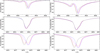 |
Fig. 2. Left-hand panels: folded (R = 50 000) model spectra showing He I 4922 Å, He I 5875 Å, and He I 6678 Å for fixed effective temperature Teff = 28000 K, fixed surface gravity log(g) = 5.60, fixed total helium abundance log n(4He+3He) ∼ −2.00, but for four different combinations of 3He and 4He abundances. The corresponding isotopic helium abundances are log n(3He) = −4.00 and log n(4He) = −2.00 (black curve), log n(3He) = −2.30 and log n(4He) = −2.30 (red curve), and log n(3He) = −2.00 and log n(4He) = −4.00 (blue curve), respectively. In addition, a model spectrum for log n(3He) = −2.05 and log n(4He) = −3.05 is shown in magenta. Right-hand panels: same as the left-hand panels, but for a fixed total helium abundance of log n(4He+3He) ∼ −1.00. |
3.2. Model grid
We determined the particular atmospheric parameters through a grid of model spectra in a four-dimensional parameter space. A multi-dimensional mesh spanned by effective temperature, surface gravity, and isotopic helium abundances was calculated for the analysis of the sdBs (see Table 3). Arbitrary parameter combinations within this mesh were approximated by linear interpolation between the calculated synthetic spectra. A detailed description on how the individual model spectra were calculated can be found in Irrgang et al. (2014). Since the parameter regime for BHB stars (PHL 25, and PHL 382) is not covered by the calculated grid for sdBs, we used small tailored meshes with the same step sizes as given in Table 3 in order to investigate them.
3.3. Spectroscopic analysis technique
The spectral analysis made use of the objective, χ2-based spectroscopic approach as described by Irrgang et al. (2014). This approach uses the whole spectrum at once. The entire wavelength range of the model spectrum, including all synthesized metal lines, can be adjusted to the real spectrum according to the Doppler effect in order to precisely determine both the radial, vrad, and the projected rotation velocity, v sin i. We set both macroturbulence zeta; and microturbulence ξ to zero, since there is no indication for additional line-broadening due to these effects in sdB stars (Geier & Heber 2012). In total, six free parameters were fitted simultaneously: Teff, log(g), log n(3He), log n(4He), vrad, and v sin i.
We used gradient methods such as mpfit in combination with non-gradient minimization algorithms such as powell and simplex in order to find the global minimum of the individual χ2 landscape, which was generally well-behaved such that the best fit was found after a relatively small number of steps. We also determined 1σ (≈68%) single parameter confidence intervals for all derived quantities.
Features that were not properly included in the models used were excluded from fitting. Such features could be cosmics, normalization problems, interstellar or telluric lines, dead or hot pixels, reduction artifacts, noise or non-overlapping diffraction orders at the end of the individual spectra, or photospheric lines with inappropriate or inaccurate atomic data.
3.4. Influence of the isotopic abundance ratio and total helium abundance on the shape of helium lines
The different isotopic line shifts strongly influence the helium line shapes and depend on both the 4He/3He isotopic abundance ratio and on the total helium abundance. The dependence on the 4He/3He ratio is demonstrated in the left-hand panels of Fig. 2, where we display different synthetic profiles for He I 4922 Å (top panel), He I 5875 Å (middle panel), and He I 6678 Å (bottom panel) calculated for Teff = 28000 K and log(g) = 5.60, that is, typical for an sdB star, but for a fixed total helium abundance of log n(4He+3He) ∼ −2.00. Because of the small isotopic shift, the shape of He I 5875 Å varies very little when the abundance ratio is varied between 4He/3He = 1/100 and 100. However, the shapes of the profiles of He I 4922 Å and He I 6678 Å change significantly. The effect of the isotopic anomaly is most pronounced for a ratio of unity, for which the He I 6678 Å line develops a hump absorption profile. For 4He/3He as high as 100, or as low as 1/100, the distortion of the line profiles by the minority isotope is invisible to the eye. Hence, we may be able to determine the isotopic ratio from He I 4922 Å and He I 6678 Å if it lies within this range. At 4He/3He = 1/10 (see the magenta line in Fig. 2), the line asymmetry remains detectable for He I 6678 Å but not for He I 4922 Å because of the smaller isotopic line shift, which means that He I 6678 Å is the more sensitive diagnostic tool. Increasing the total helium abundance generally results in stronger absorption lines with much broader line wings. This is shown in the right-hand panels of Fig. 2, where the same profiles are displayed as in the left-hand panels, but for a total helium abundance of log n(4He+3He) ∼ −1.00. Interestingly, the hump absorption profile for an abundance ratio of unity can now be identified for He I 4922 Å as well.
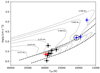 |
Fig. 3. Teff−log(g) diagram of the program stars. While known 3He sdBs from our sample are marked in black, the two 3He-enriched ESO SPY sdBs (HE 0929–0424, HE 1047–0436; see Sect. 5.3) are marked in red. The three blue dots at the cool end of the sequence represent PHL 25, PHL 382, and BD+48° 2721, highlighted with a solid circle (see Sect. 4.2 for details). The zero-age (ZAHB) and terminal-age horizontal branch (TAHB) as well as evolutionary tracks for different stellar masses but solar metallicity according to Dorman et al. (1993) are also shown with dashed and dotted lines, respectively. |
4. Atmospheric parameters and projected rotation velocities
Effective temperatures and surface gravities of the program stars were determined by fitting the calculated model spectra to the hydrogen and helium lines of the observed spectra listed in Table B.1. In addition, sharp metal lines were used for a precise determination of vrad and v sin i. Preliminary results have been reported by Schneider et al. (2017), which were based on standard ATLAS12 model atmospheres and a DETAIL/SURFACE spectrum synthesis, that is, without the modifications described in Sect. 3.1.
Effective temperatures, surface gravities, and helium abundances of the analyzed subluminous B-type stars compared to literature values.
4.1. Effective temperatures, surface gravities, and helium content
Table 4 lists the resulting effective temperatures, surface gravities, and helium abundances. Because statistical uncertainties are small, the error budget is dominated by systematic uncertainties. As suggested in the study of Lisker et al. (2005), we added systematic uncertainties of ± 2% for the effective temperatures and ± 0.1 for log(g). Given uncertainties on log n(4He+3He) in Table 4 result from Gaussian error propagation, for which we used ± 0.1 as systematic errors for log n(3He) and log n(4He), respectively. All stars are helium-deficient compared to the solar helium abundance, and except for EC 12234–2607 show typical abundances of −2.00 ≤ log n(4He+3He) ≤ −3.00. Figure 3 shows the Teff−log(g) diagram, where we compare our results to predictions of evolutionary models for the horizontal branch and beyond assuming solar metallicity and canonical masses between 0.471 M⊙ and 0.490 M⊙ (Dorman et al. 1993). Most of the analyzed 3He stars lie within the EHB band, as expected. EC 03263–6403 has already evolved beyond the helium-core burning phase as the star lies above the canonical HB. The same is true for the post-BHB star PHL 382. Consequently, EC 03263–6403 and PHL 382 should have evolved off the HB and therefore should not be burning helium at their cores. Moreover, it is worthwhile to note that Feige 36 lies below the ZAEHB, which may be explained by a lower-than-canonical mass of the star (see Kupfer et al. 2015). Most importantly, however, all 3He stars cluster in a narrow temperature strip between ∼26000 K and ∼30000 K, very similar to the results of Geier et al. (2013a).
4.2. Results from NLTE versus LTE analyses
Nine of the 3He sdB stars have been analyzed from the same high-resolution spectra used here (see Edelmann et al. 1999; Lisker et al. 2005; Geier et al. 2013a for details). All published analyses made use of the grid of metal line-blanketed LTE model atmospheres and spectral synthesis described by Heber et al. (2000). Atmospheric parameters were determined by fitting the observed hydrogen Balmer and helium lines to grids of synthetic spectra in a similar way to the analysis presented here. Previous analyses also relied on χ2 minimization, but used the codes of Napiwotzki (1999) or its variant SPAS (Hirsch 2009; see, e.g., Copperwheat et al. 2011 for a detailed description) and a solar or supersolar metallicity.
Hence, a comparison of our results to the published ones allows us to test systematic effects, that is, the cumulative impact of departures from LTE, different metal contents, and the different analysis strategies used (objective χ2 -based spectroscopic approach vs. SPAS). In Table 4 we compare our results to the published ones for the relevant stars.
No systematic differences can be identified between the two approaches for effective temperatures and surface gravities. We therefore conclude that the cumulative effect of departures from LTE, different metal contents, and the different analysis strategies is minor. All values agree to within the given uncertainties, except for BD+48° 2721 and EC 03263–6403. In the case of EC 03263–6403, we derived a lower surface gravity of log(g) = 5.21 ± 0.11 compared to literature values (5.48 ± 0.14). However, we derived a drastically lower Teff by ∼4000 K and log(g) by ∼0.57 for BD+48° 2721, although we used the same FOCES spectrum as Geier et al. (2013a). At Teff = 20 700 ± 600 K and log(g) = 4.81 ± 0.11, the atmospheric parameters of BD+48° 2721 are quite similar to those of the BHB star PHL 25. Because of this similarity, BD+48° 2721 should no longer be considered an sdB, but should be reclassified as a BHB star.
4.3. Rotational broadening
Subluminous B stars are slow rotators, unless they are spun up by a compact companion (Geier et al. 2010; Geier & Heber 2012). Projected rotational velocities have been reported for all 3He sdB stars to be low, that is, close to the detection limit, which is on the order of the typical spectral resolution element of the instrumental profile (∼5–8 km s−1). Our analysis of the metal line profiles confirms the slow rotation, which implies that rotation is irrelevant for modeling the helium line profiles to determine the isotopic abundances and the abundance ratios. However, there are two exceptions. Although apparently single, SB 290 is known to be a rapid rotator. Geier et al. (2013b) derived the projected rotation velocity from metal lines to be v sin i = 48.0 ± 2.0 km s−1. They noted, however, that the observed helium lines require a higher rotational broadening of v sin i = 58.0 ± 1.0 km s−1 to be matched by synthetic spectra. We confirm this discrepancy and discuss it in Sect. 5.4. PHL 382 also shows significant rotation, but at a lower v sin i = 12.9 ± 0.1 km s−1 than SB 290.
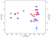 |
Fig. 4. 3He (red) and 4He (blue) abundances of the analyzed stars plotted against effective temperature. Stars showing anomalous helium line profiles (see Sect. 5.4) are marked with squares. Triangles represent 3He stars for which we were able to match the helium line profiles. In addition, both He-normal comparison stars (HD 4539 and CD-35° 15910) are marked with crosses. Their 3He upper limits (see Table 4) are not displayed. |
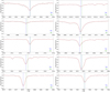 |
Fig. 5. Selected He I helium lines in the FEROS spectrum of the He-normal comparison star HD 4539. The observed spectrum (solid black line) and the best fit (solid red line) are shown. The dashed vertical lines display the 3He (green) and 4He (blue) component of the individual helium line according to the wavelengths listed in Table 1. |
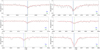 |
Fig. 7. Same as Fig. 5, but for the UVES spectrum of the formerly unclassified 3He star HE 1047–0436. The actual fit (solid red line) together with a model spectrum for the same atmospheric parameters but no 3He (dotted red line) is shown. No metals were synthesized for the latter. |
5. Isotopic helium abundances
Using the calculated model spectra presented in Sect. 3, we investigated selected He I lines in the optical spectral range for all program stars. The selection criterion for each line under investigation was its respective strength, which obviously depends on the helium abundance. In consequence, we did not use the same He I lines for the abundance analysis of each individual star. The analysis focused on a detailed synthesis of the composite helium line profiles in order to derive both isotopic abundances (4He and 3He) and the abundance ratios (4He/3He). Unfortunately, He I 7281 Å either was not covered in the spectral range of the Echelle spectrographs used (FOCES, UVES) or was truncated due to the different diffraction orders (HRS). If covered (FEROS), He I 7281 Å was too weak to be useful. In order to study the 3He anomaly in all program stars, we therefore had to rely on the strong He I 6678 Å and He I 4922 Å lines as the most important signatures for 4He/3He in the optical spectral range.
The derived 4He and 3He abundances and the isotopic abundance ratios are listed in Table 4. As expected, the changes due to the new broadening tables for He I are only minor (compare Table 4 with Table 3 in Schneider et al. 2017). There is also no systematic trend visible between the hybrid LTE/NLTE approach used here and LTE literature values regarding helium abundances.
Figure 4 summarizes the isotopic helium abundances in a Teff−log n(3He) and Teff−log n(4He) diagram for all program stars. While all 4He abundances are clearly subsolar (solar 4He abundance: log n(4He) = −1.11; Asplund et al. 2009), the 3He abundances are strongly overabundant compared to the solar 3He value of log n(3He) = −4.89 (Asplund et al. 2009).
In the following, the results on isotopic abundances and abundance ratios are presented for the He-normal comparison stars (Sect. 5.1), five known 3He sdBs (Sect. 5.2), and two from the ESO SPY survey (Sect. 5.3). We find anomalous helium line profiles for all 3He BHB and three 3He sdB stars, which are discussed in Sect. 5.4. Last, a sensitivity study in order to verify the results is provided in Sect. 5.5.
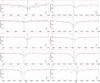 |
Fig. 8. Same as Fig. 5, but for the HRS spectrum of the 3He star PHL 25. The line cores of He I 4472 Å, He I 5875 Å, He I 6678 Å, and He I 7065 Å have been excluded from the fit because of strong stratification effects and fitting problems, as are obvious from the strong mismatch (see Sect. 5.4 for details). |
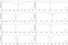 |
Fig. 9. Same as Fig. 5, but for the FOCES spectrum of the 3He star BD+48° 2721. The star shows strong helium stratification, as is obvious from the mismatch of the cores of many He I lines (see Sect. 5.4 for details). |
5.1. He-normal subdwarf B stars HD 4539 and CD-35° 15910
The fit of all suitable 4He absorption lines of HD 4539 and CD-35° 15910 is precise. As an example, Fig. 5 displays the line fits for the FEROS spectrum of HD 4539. Only small deviations between fit and observed spectrum are visible in the line wings of He I 4472 Å and He I 4922 Å, which are related to the respective forbidden component, and the predicted line cores of He I 5875 Å and He I 6678 Å, for instance, are slightly too strong. Neither comparison sdB shows any traces of 3He at all (see also Table 4). Synthetic spectra for HD 4539 and CD-35° 15910 were calculated using the solar value of log n(3He) = −4.89 (Asplund et al. 2009).
5.2. 3 He subdwarf B stars
Most of the known 3He sdB stars (EC 03263–6403, EC 14338–1445, Feige 38, PG 1710+490, and Feige 36) show fits of similar quality as the He-normal stars. Figure 6 shows the helium line fits for the FEROS spectrum of EC 03263–6403. Given the higher noise level of the spectra, these fits are satisfactory. Photospheric 3He is clearly detectable in these stars, as can be seen from the 3He and 4He abundances listed in Table 4. Feige 36 shows a balanced abundance ratio of 4He/3He ∼ 0.98, whereas for EC 03263–6403, EC 14338–1445, Feige 38, and PG 1710+490, 4He is almost absent (4He/3He < 0.25).
5.3. Two new 3He subdwarf B stars from the ESO SPY project
The most comprehensive and homogeneous sample of sdB stars for which high-resolution spectra are available emerged from the ESO SPY project (Napiwotzki et al. 2001). Overall, the sample included 76 sdBs for which UVES spectra at the ESO VLT were obtained. These spectra were analyzed by Lisker et al. (2005), but no search for the 3He anomaly has been carried out because the UVES spectra did not cover He I 7281 Å or He I 6678 Å. We revisited the list of classified sdBs in the framework of ESO SPY in order to spectroscopically study the 3He anomaly. Our focus had to be on He I 4922 Å, the strongest and most sensitive line to 3He in the spectral range of UVES (3290–6640 Å). In a first step, we preselected 26 candidates with effective temperatures between ∼27000 K and ∼31000 K typical for 3He-enriched sdBs (Geier et al. 2013a). Some of the candidates were too helium-deficient to show He I 4922 Å so that we could not investigate the 3He anomaly in those stars. We spectroscopically analyzed the remaining candidates and identified two of them as 3He-enriched sdBs by means of their isotopic abundance ratios. These stars (HE 0929–0424, HE 1047–0436; see Table 4) were classified as close binaries by Karl et al. (2006) and Napiwotzki et al. (2001), respectively. HE 0929–0424 has a semi-amplitude of K = 114.3 ± 1.4 km s−1 and a period of P = 0.4400 ± 0.0002 (d), whereas HE 1047–0436 has K = 94.0 ± 3.0 km s−1 and P = 1.21325 ± 0.00001 (d). With HE 0929–0424 and HE 1047–0436 being short-period sdB binaries, the total number of known close sdB binaries showing 3He increases to five (PG 1519+640, Feige 36, PG 0133+114, HE 0929–0424, and HE 1047–0436).
We also classified HE 2156–3927 and HE 2322–0617 as 3He-enriched sdBs in the framework of the preliminary results presented in Schneider et al. (2017). However, Lisker et al. (2005) found that both stars show features of cool companions, such as the Mg I triplet between 5167 Å and 5184 Å, which we can confirm here. In the case of HE 2156–3927, they determined the companion type to be K3, whereas the companion of HE 2322–0617 is of somewhat earlier spectral type (G9). Because the respective cool companion therefore already significantly contributes to the total flux at the spectral range of He I 4922 Å, we cannot be sure that our detection of 3He for HE 2156–3927 and HE 2322–0617 is real. Further investigations have to be conducted in order to consolidate the 3He hypothesis.
HE 0929–0424 and HE 1047–0436 have significantly higher isotopic abundance ratios than the stars discussed in Sect. 5.2 except for Feige 36 (see Table 4). This is likely a selection effect, however, because the detection limit for 4He particularly increases when He I 6678 Å is not observed, as we discuss in Sect. 5.5. In addition, the analyzed UVES spectra had lower S/N ratios than those of most other stars (see Table B.1). We managed to fit most of the helium lines for HE 0929–0424 and HE 1047–0436. As an example, the line fits for the UVES spectrum of HE 1047–0436 are displayed in Fig. 7. Based on the isotopic line shifts observable in the spectrum of the star, in particular for He I 4922 Å and He I 5015 Å, 3He enrichment is obvious.
5.4. Helium line profile anomalies and vertical stratification
We were able to fit the observed helium line profiles very precisely for the two He-normal comparison stars and five 3He sdBs. Most remarkably, however, we were unable to satisfactorily reproduce the helium line profiles in the case of all analyzed 3He-enriched BHB stars (PHL 25, BD+48° 2721, and PHL 382; see Figs. 8, 9, and A.1) and the 3He sdBs EC 03591–3232, EC 12234–2607, and SB 290 (see Figs. A.2 and A.3). A significant mismatch of the cores of many strong He I lines is obvious. Only some of the weakest He I lines could be matched satisfactorily. The most prominent cases are PHL 25 and BD+48° 2721 (see Figs. 8 and 9). To a lesser extent, discrepancies are also visible for PHL 382, EC 03591–3232, EC 12234–2607, and SB 290 (see Figs. A.1, A.2, and A.3). Because of the high rotation velocity of ∼50 km s−1 of SB 290 (see Sect. 4.3) and the line broadening it causes, a more obvious mismatch as seen for the other relevant stars might be hidden to some extent. To test this, we convolved both the observed and the synthetic spectrum of the non-rotating 3He sdB EC 03591–3232 with a rotational profile for v sin i ∼ 50 km s−1. In this way, we reproduced similarly strong mismatches in the broadened helium line profiles of the star as seen for SB 290. Therefore, we conclude that the strong line broadening in the case of SB 290 indeed hides greater shortcomings in fitting.
Because of the insufficient line matches, the resulting abundance ratios for the relevant stars in Table 4 are uncertain. Except for PHL 25 and EC 12234–2607, however, we conclude that 3He has to be the dominant isotope. Generally, we found no evidence that the stars with anomalous helium line profiles have more atmospheric helium than other program stars, although EC 03591–3232 and EC 12234–2607 belong to the most He-rich stars (see Table 4).
We calculated the entire helium line spectrum for a large variety of helium abundances, but none of them could simultaneously match both the wings and the cores of the analyzed helium absorption lines of the relevant stars. Specifically, He I 4026 Å and He I 4472 Å exhibit shallow cores in combination with unusually broad wings (see, e.g., Figs. 9 and A.1), indicating that helium is not homogeneously distributed throughout the stellar atmosphere, but instead shows a vertical abundance stratification. The shallow line cores indicate a lower-than-average helium abundance in outer atmospheric layers, where the cores are formed. The strong line wings require a higher-than-average helium abundance in deeper atmospheric layers, where the wings are formed. The farther out in the stellar atmosphere the particular helium absorption line core is formed, that is, the stronger the individual line, the poorer the reproduction of the line core (see Figs. 8, 9, A.1, A.2, and A.3). In addition to λ4026 Å and λ4472 Å, this particularly applies to λ4922 Å, λ5016 Å, λ5875 Å, λ6678 Å, and λ7065 Å and indicates that the helium abundance indeed has to be higher in deeper layers of the atmospheres than in the outer ones. The apparent discrepancy in projected rotational velocities determined from helium lines being larger than from metals in the case of SB 290 (see Sect. 4.3) can thus be explained as an effect of helium abundance stratification. Furthermore, Geier et al. (2013a) were not aware of the helium-stratified atmosphere of BD+48° 2721. Together with a different choice of helium lines for their spectral analysis, this might be the crucial factor for the discrepancy of the stellar atmospheric parameters (see Sect. 4.2).
Helium stratification has been reported for a few 3He B-type stars so far (see, e.g., Bohlender 2005). This includes B-type MS stars such as the helium-variable star aCen (Leone & Lanzafame 1997; Bohlender et al. 2010; Maza et al. 2014b), the prototype HgMn star κ Cancri (Maza et al. 2014a), and the chemically peculiar 3He star HD 185330 (Niemczura et al. 2018). Helium stratification has also been found in Feige 86, a well-studied BHB star (Bonifacio & Hack 1995; Cowley & Hubrig 2005; Cowley et al. 2009; Németh 2017), and in other chemically peculiar stars by Dworetsky (2004) and Castelli & Hubrig (2007), for example. However, this is the first time that it has been detected in subdwarf B stars.
 |
Fig. 10. Left-hand panel: best fit by eye for the line core (solid red line, log n(4He+3He) = −2.50) and the line wings (dotted red line, log n(4He+3He) = −1.79) of He I 4026 Å in the HRS spectrum of PHL 25 (solid black line). Right-hand panel: same as the left-hand panel, but for He I 4472 Å. The total helium abundances are log n(4He+3He) = −3.00 (solid red line) and log n(4He+3He) = −2.10 (dotted red line). |
In order to reproduce the observed helium line profiles and to estimate the total helium abundance, log n(4He+3He), in the outer and inner stellar atmospheres, we applied a two-component fit (see also Maza et al. 2014a). To this end, we chose the strong He I lines at λ4026 Å and λ4472 Å. Their line cores are formed farther out than their line wings. Trying to match the line cores and wings of both lines individually, we performed four fits by eye for the relevant stars, fixing the values for effective temperature, surface gravity, and projected rotation velocity determined in Sect. 4. We also estimated errors for log n(4He+3He) by varying the total helium abundance until clear mismatches in cores and wings, respectively, become obvious. Table 5 summarizes the results. As an example, Fig. 10 compares the best-fit model spectrum for the investigated helium lines to the HRS spectrum of PHL 25.
The helium abundance overall increases from outer to inner atmospheric layers of the analyzed stars (see Table 5). For He I 4026 Å, the total helium abundance increases by ∼0.15 dex for SB 290 up to ∼0.83 dex for PHL 382. Derived from He I 4472 Å, the helium abundance increases with depth even more significantly, by ∼0.46 dex for SB 290 up to ∼0.90 dex for PHL 25, EC 12234–2607, and BD+48° 2721, respectively. Depending on the individual stratified star, we hence estimate that the helium abundance increases by a factor of ∼1.4–8.0 from the outer to the inner atmosphere. This is a clear indication for an inhomogeneous distribution of helium in the atmosphere, or in other words, for vertical abundance stratification.
Last but not least, we highlight the position of the helium-stratified program stars in the Teff−log(g) plane (see Fig. 11). They populate the whole effective temperature sequence, and in contrast to the 3He sdBs, they do not cluster in a certain temperature regime.
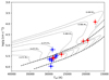 |
Fig. 11. Teff−log(g) diagram of the program stars as in Fig. 3. 3He stars from our sample showing no evidence for helium stratification are marked in blue, and the stratified 3He ones are marked in red. The zero-age (ZAHB) and terminal-age horizontal branch (TAHB) as well as evolutionary tracks for different stellar masses but solar metallicity according to Dorman et al. (1993) are also shown with dashed and dotted lines, respectively. |
5.5. Sensitivity study
Most of the known 3He sdB stars from Geier et al. (2013a) show 4He/3He < 0.25 (see Table 4). Given the range in S/N of the observations, what are the detection limits for 4He?
We added Gaussian noise to spectra computed with the parameters and S/N ratios given in Tables 4 and B.1 for three program stars: EC03263–6403 = Model I, BD+48° 2721 = Model II, and HE 1047–0436 = Model III. BD+48° 2721 was chosen for its high S/N ratio (∼84; see Table B.1), EC 03263–6403 for its low isotopic ratio (4He/3He ∼ 0.01, see Table 4), and HE 1047–0436 for having the lowest 4He abundance of the 3He ESO SPY sdBs (where the sensitive He I 6678 Å line has not been observed; see also Table 4).
The Gaussian noise was simulated using samples (p), drawn from a parameterized normal distribution centered around zero (mean value μ = 0) and with a standard deviation of one (σ = 1). The fluxes of the individual mock spectra, Fmock, then were calculated from model fluxes, Fmodel, according to the following formula:
 (1)
(1)
Here, S/N is the individual signal-to-noise ratio. We chose different values for S/N: 1) the original S/N of the individual observed spectra; 2) S/N = 100; 3) S/N = 200; and 4) S/N = 300. We simultaneously fitted effective temperature, surface gravity, and both isotopic helium abundances, making use of the same analysis technique as presented in Sect. 3.3.
5.5.1. Detectability and error estimation
The results of the sensitivity study for the three models together with those of the abundance analysis are shown in Table 6. In the following, we highlight three important results.
First, we are able to reproduce the results of the previous abundance analysis. This confirms that the abundances given in Table 4 are reliable detections of the small traces of 4He. Values and uncertainties for log n(4He) and log n(3He) derived from mock spectra are overall in good agreement with the observed ones if the same S/N and the same number of investigated helium lines are used. Increasing the S/N ratio, however, results in a significant improvement of accuracy.
Second, if the strong and sensitive He I 6678 Å line is ignored, we are not able to reproduce the observed 4He abundances for EC 03263–6403 and BD+48° 2721. In particular, this results in large statistical uncertainties on log n(4He), even for better S/N. Hence, it is not possible to determine log n(4He) of the 4He-deficient sdB star EC 03263–6403 without He I 6678 Å.
Last, we also derived similar isotopic helium abundances and statistical uncertainties from mock spectra as from the previous abundance analysis in the case of HE 1047–0436, that is, for the most 4He-deficient but 3He-enriched sdB star from the ESO SPY project (see Table 4). We simulated the case of the analyzed UVES spectra in which He I 6678 Å as the most important signature for 4He/3He was also not available for investigation. This result substantiates the discovery of HE 1047–0436 as a 3He-enriched sdB. Adding observations of He I 6678 Å (and He I 10830 Å, see Sect. 5.5.2) would still significantly improve the accuracy of the analysis and might reveal other unclassified 3He sdBs in the ESO SPY sample at lower 4He/3He ratios.
In addition, it is worthwhile to deduce a detection limit for 3He. Although He I 6678 Å is not observed for HE 1047–0436 and the S/N is mediocre, Fig. 7 demonstrates that the 3He anomaly is detectable at an 4He/3He abundance ratio as high as ∼0.91 even for such poor data. In consequence, we conclude that all other cases where the abundance ratio is lower than ∼0.91 are indeed reliable detections of 3He, even if the 3He abundance is as low as log n(3He) ∼ −3.10, as in the case of EC 14338–1445. Hence, the latter is a reliable upper limit for the detection limit for 3He. HE 0929–0424 has an even higher abundance ratio (4He/3He ∼ 2.51) than HE 1047–0436, but at the same time shows significantly more helium (see Table 4). Thus, the discovery of HE 0929–0424 as a 3He-enriched sdB is reliable as well.
Results of the sensitivity study.
Influence of He I 10830 Å on the sensitivity study for BD+48° 2721.
5.5.2. Infrared He I 10830 Å line
He I 10830 Å in the near-infrared is known to show the largest isotopic line shift of ∼1.32 Å, that is, more than twice as large as for He I 6678 Å ( ∼0.50 Å). Thus, the He I 10830 Å line should improve the detectability of 3He and in turn the sensitivity to 4He/3He significantly. As He I 5875 Å and He I 6678 Å, this line is strongly affected by departures from LTE. However, the helium model atom used here in combination with the hybrid LTE/NLTE approach have been shown to be appropriate to match the observed line profiles in early B-type MS stars well (Przybilla 2005). Hence, we included He I 10830 Å into the sensitivity study for BD+48° 2721 (see Table 7) in order to test its influence on the derived 4He/3He abundance ratio.
He I 10830 Å indeed particularly leads to a better accuracy in determining both isotopic abundances for a given S/N (compare the results in Table 7 to those in Table 6). Both isotopic abundances are already well determined if He I 6678 Å as well as He I 10830 Å are available and the S/N ratio is on the order of ∼85. An even higher S/N decreases the derived statistical uncertainties on both isotopic abundances if He I 10830 Å is included.
6. Conclusion and outlook
We carried out a quantitative spectral analysis of 13 subluminous B stars that show the 3He anomaly (three BHBs, eight known sdBs, and two newly discovered sdBs from the ESO Supernova Ia Progenitor Survey), as well as of two prototypical He-normal sdBs for reference, making use of high-quality optical spectra and a grid of synthetic spectra calculated in a hybrid LTE/NLTE approach based on modified versions of the model atmosphere code ATLAS12 and the NLTE line formation and synthesis codes DETAIL and SURFACE. Well-tested model atoms were supplemented by a 3He model atom from Maza et al. (2014a).
We redetermined effective temperatures, surface gravities, and helium abundances of nine stars previously analyzed from the same spectra but using LTE model atmospheres, different metal contents, and a different minimization procedure to determine the best fit. In general, the results were found to be consistent for all but one program star (BD+48° 2721), indicating that systematic effects by the cumulative impact of departures from LTE, different metal contents, and the different analysis strategies are small. However, BD+48° 2721 is much cooler than previously deduced, and was therefore reclassified as a BHB star.
Isotopic abundance ratios, 4He/3He, were determined from the helium line spectra. Both He I 6678 Å and He I 5875 Å play a crucial role because they show the largest and smallest isotopic line shift, respectively. However, these lines are known to be strengthened by departures from LTE, in particular He I 6678 Å, which requires an appropriately detailed atomic model and sophisticated line broadening tables. We verified our synthetic spectra against the benchmark sdB stars HD 4539 and CD-35° 15910.
As expected, 4He is almost absent (4He/3He < 0.25) in most of the known 3He sdB stars from Geier et al. (2013a). We identified the 3He anomaly in the stellar atmospheres of HE 0929–0424 and HE 1047–0436, resulting in 4He/3He ∼ 2.51 and 4He/3He ∼ 0.91, respectively. This substantiates the helium abundance results for the known 3He stars. The interesting question arises whether there is a continuum of 3He-enriched sdBs/BHBs at higher abundance ratios (4He/3He ∼ 1.0–3.0), which could be answered from a homogenous sample with excellent data. Such a sample may be the one of Geier et al. (2013a), who examined 44 bright sdB stars that have been observed at high spectral resolution and good S/N, covering He I 6678 Å (e.g., with FEROS) with a sharp eye on the isotopic anomaly. The sample is somewhat biased, however, because the previously known 3He sdBs were included a priori. All new 3He sdBs found by Geier et al. (2013a) have very low 4He abundances (log n(4He) ≲ −3.30), except for EC 12234–2607. A larger unbiased sample is needed in order to draw sound conclusions on a potential continuum.
Anomalous helium line profiles (broad wings, shallow cores) were found in all three BHB (PHL 25, PHL 382, and BD+48° 2721) and in three of the 3He sdB stars (EC 03591–3232, EC 12234–2607, and SB 290). This phenomenon can be explained by vertical stratification of the atmospheres. We estimate that the helium abundance increases from the outer atmospheric layers, where the cores of strong helium lines form, to the deeper ones, where the line wings form, by factors ranging from about 1.4 in the case of the sdB SB 290 to a factor of 8.0 in the case of the BHB star BD+48° 2721. Such a layered distribution of helium has been found previously in late B-type stars of peculiar chemical composition as well as in other BHB stars, but this is the first time that helium stratification is reported for sdB stars. A particularly interesting case is SB 290, because it is the only rapidly rotating sdB in the sample. Geier et al. (2013b) derived v sin i = 48.0 ± 2.0 km s−1 from metal, but v sin i = 58.0 ± 1.0 km s−1 from helium lines. We confirmed this discrepancy and traced it back to the anomalous helium line profiles. The projected rotational velocity of v sin i = 58.0 ± 1.0 km s−1 derived from helium lines by Geier et al. (2013b) is therefore overestimated because of vertical helium abundance stratification.
The simplest way to carry out a quantitative spectral analysis of the stratification profile is to make use of a smoothed step function (see, Farthmann et al. 1994), which sets the helium abundance in the outer atmospheric layers to a lower level than farther in. In this way, the optical depth at which the change in helium abundance occurs can also be identified. As an example, stratification analyses have been carried out successfully for carbon and nitrogen in the post-HB star HD 76431 by Khalack et al. (2014) and for nitrogen, sulfur, titanium, and in particular for iron, in BHB stars by Khalack et al. (2007, 2008, 2010) and LeBlanc et al. (2010). The strategy to derive the stratified helium abundance profile throughout the photosphere with the hybrid LTE/NLTE approach was reported in Maza et al. (2014a), who tested it successfully on κ Cancri.
The 3He anomaly for MS stars is restricted to a narrow temperature strip of 14000 K ≲ Teff ≲ 21000 K (Sargent & Jugaku 1961; Hartoog & Cowley 1979). The same is true for sdB stars, but at hotter temperatures (26000 K ≲ Teff ≲ 30000 K). Otherwise, no correlation can be found. The anomaly occurs for single as well as for close binary sdBs (PG 1519+640, Feige 36, PG 0133+114, HE 0929–0424, and HE 1047–0436). We also found evidence that it occurs for objects that have evolved off the canonical horizontal branch, as in the case of EC 03263–6403 and PHL 382.
The 3He isotopic anomaly was previously considered to be a rare phenomenon. Although many sdB stars have been analyzed by means of high-resolution spectra, observations of the crucial He I 6678 Å line are lacking in many cases, in particular for the largest homogeneous sdB sample from the ESO SPY project (Lisker et al. 2005). The fraction of 3He stars among sdBs could be best constrained from high-resolution spectroscopy of the He I 6678 Å line. However, even more promising for investigating the isotopic anomaly would be observations of the near-infrared helium line, He I 10830 Å, which now becomes possible with modern spectrographs.
Acknowledgments
D. S. was supported by the Deutsche Forschungsgemeinschaft (DFG) under grant HE 1356/70-1. M. F. N. acknowledges support by the Austrian Science Fund (FWF) in the form of a Lise-Meitner Fellowship under project number N-1868-NBL. We thank S. Geier and H. Edelmann for sharing their data with us. We wish to thank the anonymous referee for providing us with a number of detailed comments that greatly improved the clarity of this manuscript. We made use of ISIS functions provided by ECAP/Remeis observatory and MIT (http://www.sternwarte.uni-erlangen.de/isis/). We thank J. E. Davis for the development of the slxfig module, which has been used to prepare part of the figures in this work. For the other part matplotlib (Hunter 2007) and NumPy (van der Walt et al. 2011) were used. Based on observations at the La Silla Observatory of the European Southern Observatory (ESO) and on observations made at the Centro Astronómico Hispano Alemán (CAHA) at Calar Alto, operated jointly by the Max-Planck-Institut für Astronomie and the Instituto de Astrofísica de Andalucía (CSIC). Based on observations made at the McDonald Observatory in Austin operated by the University of Texas and on observations conducted at the W. M. Keck Observatory on Hawaii.
There is no uniform classification of PHL 382. First, the star was classified as a BHB star by Heber (1987). However, it might also be an evolved low-mass star that has left the He-core burning phase (post-BHB star). Finally, it could also be an MS star, as suggested by Kilkenny & van Wyk (1990) and Dufton et al. (1993) because of its low surface gravity. For the work at hand, we initially make use of the classification of Heber (1987) and call PHL 382 a BHB star. This classification is further discussed in Sect. 4.1.
Przybilla et al. (2010) provided a hybrid LTE/NLTE study of the fast halo BHB star SDSSJ153935.67+023909.8 in order to constrain the mass of the Galactic dark matter halo. By making use of the same hybrid approach, Marino et al. (2014) analyzed HB/BHB stars in the globular cluster NGC 2808. However, all previously investigated BHBs are cooler than those in our sample, which are PHL 25 and PHL 382.
References
- Asplund, M., Grevesse, N., Sauval, A. J., et al. 2009, ARA&A, 47, 481 [NASA ADS] [CrossRef] [Google Scholar]
- Atutov, S. N. 1986, Phys. Lett. A, 119, 121 [NASA ADS] [CrossRef] [Google Scholar]
- Auer, L. H., & Mihalas, D. 1973, ApJS, 25, 433 [NASA ADS] [CrossRef] [Google Scholar]
- Babel, J. 1996, A&A, 309, 867 [NASA ADS] [Google Scholar]
- Beauchamp, A., Wesemael, F., & Bergeron, P. 1997, ApJ, 108, 559 [NASA ADS] [Google Scholar]
- Becker, S. R. 1998, ASP Conf. Ser., 131, 137 [NASA ADS] [Google Scholar]
- Becker, S. R., & Butler, K. 1988, A&A, 201, 232 [NASA ADS] [Google Scholar]
- Bohlender, D. 2005, EAS Pub. Ser., 17, 83 [CrossRef] [Google Scholar]
- Bohlender, D. A., Rice, J. B., & Hechler, P. 2010, A&A, 520, A44 [NASA ADS] [CrossRef] [EDP Sciences] [Google Scholar]
- Bonifacio, P. C. F., & Hack, M. 1995, A&AS, 110, 441 [NASA ADS] [Google Scholar]
- Butler, K., & Giddings, J. R. 1985, in Newsletter of Analysis of Astronomical Spectra, No. 9 (Univ. London) [Google Scholar]
- Castelli, F., & Hubrig, S. 2007, A&A, 475, 1041 [NASA ADS] [CrossRef] [EDP Sciences] [Google Scholar]
- Copperwheat, C. M., Morales-Rueda, L., Marsh, T. R., et al. 2011, MNRAS, 415, 1381 [NASA ADS] [CrossRef] [Google Scholar]
- Cowley, C. R., & Hubrig, S. 2005, A&A, 432, L21 [NASA ADS] [CrossRef] [EDP Sciences] [Google Scholar]
- Cowley, C. R., Hubrig, S., & González, J. F. 2009, MNRAS, 396, 485 [NASA ADS] [CrossRef] [Google Scholar]
- Dekker, H., D’Odorico, S., Kaufer, A., et al. 2000, in Optical and IR Telescope Instrumentation and Detectors, eds. M. Iye, & A. F. Moorwood, Proc. SPIE, 4008, 534 [Google Scholar]
- Dimitrijevic, M. S., & Sahal-Brechot, S. 1990, A&AS, 82, 519 [NASA ADS] [Google Scholar]
- Dorman, B., Rood, R. T., & O’Connell, R. W. 1993, ApJ, 419, 596 [CrossRef] [Google Scholar]
- Dufton, P. L., Conlon, E. S., Keenan, F. P., et al. 1993, A&A, 269, 201 [NASA ADS] [Google Scholar]
- Dworetsky, M. M. 2004, in The A-Star Puzzle, eds. Zverko, J. Ziznovsky, J. Adelman, S. J., & Weiss, W. W., IAU Symp., 224, 727 [NASA ADS] [CrossRef] [Google Scholar]
- Edelmann, H., Heber, U., Napiwotzki, R., et al. 1997, Astron. Ges. Abstract Ser., 13, 206 [NASA ADS] [Google Scholar]
- Edelmann, H., Heber, U., Napiwotzki, R., et al. 1999, in 11th European Workshop on White Dwarfs, eds. S.-E. Solheim, & E. G. Meistas (San Francisco: Astronomical Society of the Pacific), ASP Conf. Ser., 169, 546 [NASA ADS] [Google Scholar]
- Edelmann, H., Heber, U., & Napiwotzki, R. 2001, Astron. Nachr., 322, 401 [NASA ADS] [CrossRef] [Google Scholar]
- Edelmann, H., Heber, U., Lisker, T., et al. 2004, Ap&SS, 291, 315 [NASA ADS] [CrossRef] [Google Scholar]
- Edelmann, H., Heber, U., Altmann, M., et al. 2005, A&A, 442, 1023 [NASA ADS] [CrossRef] [EDP Sciences] [Google Scholar]
- Farthmann, M., Dreizler, S., Heber, U., et al. 1994, A&A, 291, 919 [NASA ADS] [Google Scholar]
- Fontaine, G., & Chayer, P. 1997, in The Third Conference on Faint Blue Stars, eds. A. G. D. Philip, J. Liebert, R. A. Saffer, & D. S. Hayes, 169 [Google Scholar]
- Fred, M., Tomkins, F. S., Brody, J. K., et al. 1951, Phys. Rev., 82, 406 [NASA ADS] [CrossRef] [Google Scholar]
- Geier, S., & Heber, U. 2012, A&A, 543, A149 [NASA ADS] [CrossRef] [EDP Sciences] [Google Scholar]
- Geier, S., Nesslinger, S., Heber, U., et al. 2007, A&A, 464, 299 [NASA ADS] [CrossRef] [EDP Sciences] [Google Scholar]
- Geier, S., Heber, U., Podsiadlowski, P., et al. 2010, A&A, 519, A25 [NASA ADS] [CrossRef] [EDP Sciences] [Google Scholar]
- Geier, S., Heber, U., Edelmann, H., et al. 2013a, A&A, 557, A122 [NASA ADS] [CrossRef] [EDP Sciences] [Google Scholar]
- Geier, S., Heber, U., Heuser, C., et al. 2013b, A&A, 551, L4 [NASA ADS] [CrossRef] [EDP Sciences] [Google Scholar]
- Giddings, J. R. 1981, PhD Thesis, University of London, UK [Google Scholar]
- Green, P. J. 2000, IAU Symp., 177, 27 [NASA ADS] [Google Scholar]
- Greenstein, G. S. 1967, Nature, 213, 871 [NASA ADS] [CrossRef] [Google Scholar]
- Hartoog, M. R. 1979, ApJ, 231, 161 [NASA ADS] [CrossRef] [Google Scholar]
- Hartoog, M. R., & Cowley, A. P. 1979, ApJ, 228, 229 [NASA ADS] [CrossRef] [Google Scholar]
- Heber, U. 1987, MitAG, 70, 79 [NASA ADS] [Google Scholar]
- Heber, U. 2009, ARA&A, 47, 211 [NASA ADS] [CrossRef] [Google Scholar]
- Heber, U. 2016, PASP, 128 [Google Scholar]
- Heber, U., & Edelmann, H. 2004, Ap&SS, 291, 341 [NASA ADS] [CrossRef] [Google Scholar]
- Heber, U., Bade, N., Jordan, S., et al. 1993, A&A, 267, L31 [NASA ADS] [Google Scholar]
- Heber, U., Reid, I. N., & Werner, K. 2000, A&A, 363, 198 [NASA ADS] [Google Scholar]
- Hirsch, H. A. 2009, PhD Thesis, Friedrich-Alexander University Erlangen-Nürnberg, Germany [Google Scholar]
- Hubeny, I., Hummer, D. G., & Lanz, T. 1994, A&A, 282, 151 [NASA ADS] [Google Scholar]
- Hughes, D. S., & Eckart, C. 1930, Phys. Rev., 36, 694 [NASA ADS] [CrossRef] [Google Scholar]
- Hunter, J. D. 2007, Comput. Sci. Eng., 9, 90 [Google Scholar]
- Irrgang, A., Przybilla, N., Heber, U., et al. 2014, A&A, 565, A63 [NASA ADS] [CrossRef] [EDP Sciences] [Google Scholar]
- Karl, C., Heber, U., Jeffery, S., et al. 2006, Baltic Astron., 15, 151 [NASA ADS] [Google Scholar]
- Kaufer, A., Stahl, O., Tubbesing, S., et al. 1999, The Messenger, 95, 8 [Google Scholar]
- Khalack, V. R., Leblanc, F., Bohlender, D., Wade, G. A., & Behr, B. B. 2007, A&A, 466, 667 [NASA ADS] [CrossRef] [EDP Sciences] [Google Scholar]
- Khalack, V. R., Leblanc, F., Behr, B. B., Wade, G. A., & Bohlender, D. 2008, A&A, 477, 641 [NASA ADS] [CrossRef] [EDP Sciences] [Google Scholar]
- Khalack, V., LeBlanc, F., & Behr, B. B. 2010, MNRAS, 407, 1767 [NASA ADS] [CrossRef] [Google Scholar]
- Khalack, V., Yameogo, B., LeBlanc, F., et al. 2014, MNRAS, 445, 4086 [NASA ADS] [CrossRef] [Google Scholar]
- Kilkenny, D., & van Wyk, F. 1990, MNRAS, 244, 727 [NASA ADS] [Google Scholar]
- Kupfer, T., Geier, S., Heber, U., et al. 2015, A&A, 576, A44 [NASA ADS] [CrossRef] [EDP Sciences] [Google Scholar]
- Kurucz, R. L. 1996, in Model Atmospheres and Spectrum Synthesis, eds. S. J. Adelman, F. Kupka, & W. W. Weiss, 108, 160 [Google Scholar]
- Langer, N. 2012, ARA&A, 50, 107 [NASA ADS] [CrossRef] [Google Scholar]
- Latour, M., Heber, U., Irrgang, A., et al. 2016, A&A, 585, A115 [NASA ADS] [CrossRef] [EDP Sciences] [Google Scholar]
- LeBlanc, F., & Michaud, G. 1993, ApJ, 408, 251 [NASA ADS] [CrossRef] [Google Scholar]
- LeBlanc, F., Hui-Bon-Hoa, A., & Khalack, V. R. 2010, MNRAS, 409, 1606 [NASA ADS] [CrossRef] [Google Scholar]
- Leone, F., & Lanzafame, A. C. 1997, A&A, 320, 893 [NASA ADS] [Google Scholar]
- Lisker, T., Heber, U., Napiwotzki, R., et al. 2005, A&A, 430, 223 [NASA ADS] [CrossRef] [EDP Sciences] [Google Scholar]
- Marino, A. F., Milone, A. P., Przybilla, N., et al. 2014, MNRAS, 437, 1609 [NASA ADS] [CrossRef] [Google Scholar]
- Maza, N. L., Nieva, M. F., & Przybilla, N. 2014a, A&A, 572, A112 [NASA ADS] [CrossRef] [EDP Sciences] [Google Scholar]
- Maza, N. L., Nieva, M. F., Przybilla, N., et al. 2014b, Rev. Mex. Astron. Astrofis. Conf. Ser., 44, 159 [Google Scholar]
- Michaud, G., & Tutukov, A. V. 1991, IAU Symp., 145 [Google Scholar]
- Michaud, G., Martel, A., Montmerle, T., et al. 1979, ApJ, 234, 206 [NASA ADS] [CrossRef] [Google Scholar]
- Michaud, G., Richer, J., & Richard, O. 2008, ApJ, 675, 1223 [NASA ADS] [CrossRef] [Google Scholar]
- Michaud, G., Richer, J., & Richard, O. 2011, A&A, 529, A60 [NASA ADS] [CrossRef] [EDP Sciences] [Google Scholar]
- Michaud, G., Alecian, G., & Richer, J. 2015, Atomic Diffusion in Stars (Switzerland: Springer International Publishing), 1 [Google Scholar]
- Morales-Rueda, L., Marsh, T. R., North, R. C., et al. 2003a, in White Dwarfs (Dordrecht: Kluwer Academic Publishers), NATO Science Series II, 105, 57 [Google Scholar]
- Morales-Rueda, L., Maxted, P. F. L., Marsh, T. R., et al. 2003b, MNRAS, 338, 752 [NASA ADS] [CrossRef] [Google Scholar]
- Moran, C., Maxted, P., Marsh, T. R., et al. 1999, MNRAS, 304, 535 [NASA ADS] [CrossRef] [Google Scholar]
- Morel, T., & Butler, K. 2008, A&A, 487, 307 [NASA ADS] [CrossRef] [EDP Sciences] [Google Scholar]
- Morel, T., Butler, K., Aerts, C., et al. 2006, A&A, 457, 651 [NASA ADS] [CrossRef] [EDP Sciences] [Google Scholar]
- Napiwotzki, R. 1999, A&A, 350, 101 [Google Scholar]
- Napiwotzki, R., Christlieb, N., Drechsel, H., et al. 2001, Astron. Nachr., 322, 411 [NASA ADS] [CrossRef] [Google Scholar]
- Naslim, N., Jeffery, C. S., Hibbert, A., et al. 2013, MNRAS, 434, 1920 [NASA ADS] [CrossRef] [Google Scholar]
- Németh, P. 2017, Open Astron., 26, 280 [NASA ADS] [Google Scholar]
- Niemczura, E., Vennes, S., Ró˙za´nski, T., et al. 2018, Contrib. Astron. Obs. Skalnaté Pleso, 48, 287 [NASA ADS] [Google Scholar]
- Nieva, M. F., & Przybilla, N. 2006, ApJ, 639, L39 [NASA ADS] [CrossRef] [Google Scholar]
- Nieva, M. F., & Przybilla, N. 2007, A&A, 467, 295 [NASA ADS] [CrossRef] [EDP Sciences] [Google Scholar]
- Nieva, M. F., & Przybilla, N. 2008, A&A, 481, 199 [NASA ADS] [CrossRef] [EDP Sciences] [Google Scholar]
- Nieva, M. F., & Przybilla, N. 2012, A&A, 539, A143 [NASA ADS] [CrossRef] [EDP Sciences] [Google Scholar]
- Pfeiffer, M. J., Frank, C., Baumüller, D., et al. 1998, A&AS, 130, 381 [NASA ADS] [CrossRef] [EDP Sciences] [Google Scholar]
- Przybilla, N. 2005, A&A, 443, 293 [NASA ADS] [CrossRef] [EDP Sciences] [Google Scholar]
- Przybilla, N., & Butler, K. 2001, A&A, 379, 955 [NASA ADS] [CrossRef] [EDP Sciences] [Google Scholar]
- Przybilla, N., & Butler, K. 2004, ApJ, 609, 1181 [NASA ADS] [CrossRef] [Google Scholar]
- Przybilla, N., Butler, K., Becker, S. R., et al. 2001, A&A, 369, 1009 [NASA ADS] [CrossRef] [EDP Sciences] [Google Scholar]
- Przybilla, N., Butler, K., Heber, U., et al. 2005, A&A, 443, L25 [NASA ADS] [CrossRef] [EDP Sciences] [Google Scholar]
- Przybilla, N., Butler, K., Becker, S. R., et al. 2006a, A&A, 445, 1099 [NASA ADS] [CrossRef] [EDP Sciences] [Google Scholar]
- Przybilla, N., Nieva, M. F., & Edelmann, H. 2006b, Baltic Astron., 15, 107 [NASA ADS] [Google Scholar]
- Przybilla, N., Tillich, A., Heber, U., et al. 2010, ApJ, 718, 37 [NASA ADS] [CrossRef] [Google Scholar]
- Przybilla, N., Nieva, M. F., & Butler, K. 2011, J. Phys. Conf. Ser., 328, 012015 [NASA ADS] [CrossRef] [Google Scholar]
- Quievy, D., Charbonneau, P., Michaud, G., et al. 2009, A&A, 500, 1163 [NASA ADS] [CrossRef] [EDP Sciences] [Google Scholar]
- Saffer, R. A., Livio, M., & Yungelson, L. R. 1998, ApJ, 502, 394 [NASA ADS] [CrossRef] [Google Scholar]
- Sargent, A. W. L. W., & Jugaku, J. 1961, ApJ, 134, 777 [NASA ADS] [CrossRef] [Google Scholar]
- Schneider, D., Irrgang, A., Heber, U., et al. 2017, Open Astron., 26, 139 [NASA ADS] [CrossRef] [Google Scholar]
- Smith, K. C. 1996, Ap&SS, 237, 77 [NASA ADS] [CrossRef] [Google Scholar]
- Tremblay, P.-E., & Bergeron, P. 2009, ApJ, 696, 1755 [NASA ADS] [CrossRef] [Google Scholar]
- Tull, R. G. 1998, Proc. SPIE, 3355, 387 [NASA ADS] [CrossRef] [Google Scholar]
- van der Walt, S., Colbert, S. C., & Varoquaux, G. 2011, Comput. Sci. Eng., 13, 22 [CrossRef] [Google Scholar]
- Vauclair, S. 1975, A&A, 45, 233 [NASA ADS] [Google Scholar]
- Vauclair, S., Michaud, G., & Charland, Y. 1974, A&A, 31, 381 [NASA ADS] [Google Scholar]
- Vogt, S. S., Allen, S. L., Bigelow, B. C., et al. 1994, in Instrumentation in Astronomy VIII, eds. D. L. Crawford, & E. R. Craine, Proc. SPIE, 2198, 362 [Google Scholar]
- Vrancken, M., Butler, K., & Becker, S. R. 1996, A&A, 311, 661 [NASA ADS] [Google Scholar]
- Werner, K., & Herwig, F. 2006, PASP, 118, 183 [NASA ADS] [CrossRef] [Google Scholar]
Appendix A: Helium line fits
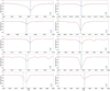 |
Fig. A.1. Same as Fig. 5, but for the FEROS spectrum of the 3He star PHL 382. The star shows strong helium stratification, as is obvious from the mismatch of the cores of many He I lines (see Sect. 5.4 for details). |
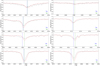 |
Fig. A.2. Same as Fig. 5, but for the FEROS spectrum of the 3He star EC 03591–3232. The star shows helium stratification, as is obvious from the mismatch of the cores of several strong He I lines (see Sect. 5.4 for details). |
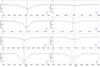 |
Fig. A.3. Same as Fig. 5, but for the FEROS spectrum of the 3He star SB 290. The star rotates, but also shows significant mismatches in the strongest He I lines, which points toward vertical helium stratification (see Sect. 5.4 for details). |
Appendix B: Target sample and data
Target sample and data of the subluminous B-type program stars.
All Tables
Transitions and isotopic shifts Δλ := λ(3He) − λ(4He) of selected He I lines in the near-ultraviolet, optical, and near-infrared spectral range up to principal quantum number n = 8.
Model grid used for the quantitative spectral analysis of sdBs.\label{model grid used for the quantitative spectral analysis of sdBs.
Effective temperatures, surface gravities, and helium abundances of the analyzed subluminous B-type stars compared to literature values.
All Figures
|
Fig. 1. Left-hand panel: model spectra for He I 6678 Å calculated in LTE (black curve) and NLTE (red and blue curve) for Teff = 28000 K, log(g) = 5.60, and log(y) = −2.00. He I 6678 Å is clearly strongly affected by NLTE effects. While the red model is based on “old” Stark broadening tables for hydrogen and He I (Dimitrijevic & Sahal-Brechot 1990), the blue model uses “new” broadening tables from Beauchamp et al. (1997). Right-hand panel: same as the left-hand panel, but zoomed-in. The difference between the “old” (red curve) and “new” (blue curve) model is marginal, but sufficient in order to explain small deviations in atmospheric parameter determination (see Sect. 3.1 for details). |
| In the text | |
|
Fig. 2. Left-hand panels: folded (R = 50 000) model spectra showing He I 4922 Å, He I 5875 Å, and He I 6678 Å for fixed effective temperature Teff = 28000 K, fixed surface gravity log(g) = 5.60, fixed total helium abundance log n(4He+3He) ∼ −2.00, but for four different combinations of 3He and 4He abundances. The corresponding isotopic helium abundances are log n(3He) = −4.00 and log n(4He) = −2.00 (black curve), log n(3He) = −2.30 and log n(4He) = −2.30 (red curve), and log n(3He) = −2.00 and log n(4He) = −4.00 (blue curve), respectively. In addition, a model spectrum for log n(3He) = −2.05 and log n(4He) = −3.05 is shown in magenta. Right-hand panels: same as the left-hand panels, but for a fixed total helium abundance of log n(4He+3He) ∼ −1.00. |
| In the text | |
|
Fig. 3. Teff−log(g) diagram of the program stars. While known 3He sdBs from our sample are marked in black, the two 3He-enriched ESO SPY sdBs (HE 0929–0424, HE 1047–0436; see Sect. 5.3) are marked in red. The three blue dots at the cool end of the sequence represent PHL 25, PHL 382, and BD+48° 2721, highlighted with a solid circle (see Sect. 4.2 for details). The zero-age (ZAHB) and terminal-age horizontal branch (TAHB) as well as evolutionary tracks for different stellar masses but solar metallicity according to Dorman et al. (1993) are also shown with dashed and dotted lines, respectively. |
| In the text | |
|
Fig. 4. 3He (red) and 4He (blue) abundances of the analyzed stars plotted against effective temperature. Stars showing anomalous helium line profiles (see Sect. 5.4) are marked with squares. Triangles represent 3He stars for which we were able to match the helium line profiles. In addition, both He-normal comparison stars (HD 4539 and CD-35° 15910) are marked with crosses. Their 3He upper limits (see Table 4) are not displayed. |
| In the text | |
|
Fig. 5. Selected He I helium lines in the FEROS spectrum of the He-normal comparison star HD 4539. The observed spectrum (solid black line) and the best fit (solid red line) are shown. The dashed vertical lines display the 3He (green) and 4He (blue) component of the individual helium line according to the wavelengths listed in Table 1. |
| In the text | |
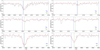 |
Fig. 6. Same as Fig. 5, but for the FEROS spectrum of the 3He star EC 03263–6403. |
| In the text | |
|
Fig. 7. Same as Fig. 5, but for the UVES spectrum of the formerly unclassified 3He star HE 1047–0436. The actual fit (solid red line) together with a model spectrum for the same atmospheric parameters but no 3He (dotted red line) is shown. No metals were synthesized for the latter. |
| In the text | |
|
Fig. 8. Same as Fig. 5, but for the HRS spectrum of the 3He star PHL 25. The line cores of He I 4472 Å, He I 5875 Å, He I 6678 Å, and He I 7065 Å have been excluded from the fit because of strong stratification effects and fitting problems, as are obvious from the strong mismatch (see Sect. 5.4 for details). |
| In the text | |
|
Fig. 9. Same as Fig. 5, but for the FOCES spectrum of the 3He star BD+48° 2721. The star shows strong helium stratification, as is obvious from the mismatch of the cores of many He I lines (see Sect. 5.4 for details). |
| In the text | |
|
Fig. 10. Left-hand panel: best fit by eye for the line core (solid red line, log n(4He+3He) = −2.50) and the line wings (dotted red line, log n(4He+3He) = −1.79) of He I 4026 Å in the HRS spectrum of PHL 25 (solid black line). Right-hand panel: same as the left-hand panel, but for He I 4472 Å. The total helium abundances are log n(4He+3He) = −3.00 (solid red line) and log n(4He+3He) = −2.10 (dotted red line). |
| In the text | |
|
Fig. 11. Teff−log(g) diagram of the program stars as in Fig. 3. 3He stars from our sample showing no evidence for helium stratification are marked in blue, and the stratified 3He ones are marked in red. The zero-age (ZAHB) and terminal-age horizontal branch (TAHB) as well as evolutionary tracks for different stellar masses but solar metallicity according to Dorman et al. (1993) are also shown with dashed and dotted lines, respectively. |
| In the text | |
|
Fig. A.1. Same as Fig. 5, but for the FEROS spectrum of the 3He star PHL 382. The star shows strong helium stratification, as is obvious from the mismatch of the cores of many He I lines (see Sect. 5.4 for details). |
| In the text | |
|
Fig. A.2. Same as Fig. 5, but for the FEROS spectrum of the 3He star EC 03591–3232. The star shows helium stratification, as is obvious from the mismatch of the cores of several strong He I lines (see Sect. 5.4 for details). |
| In the text | |
|
Fig. A.3. Same as Fig. 5, but for the FEROS spectrum of the 3He star SB 290. The star rotates, but also shows significant mismatches in the strongest He I lines, which points toward vertical helium stratification (see Sect. 5.4 for details). |
| In the text | |
Current usage metrics show cumulative count of Article Views (full-text article views including HTML views, PDF and ePub downloads, according to the available data) and Abstracts Views on Vision4Press platform.
Data correspond to usage on the plateform after 2015. The current usage metrics is available 48-96 hours after online publication and is updated daily on week days.
Initial download of the metrics may take a while.