| Issue |
A&A
Volume 618, October 2018
|
|
|---|---|---|
| Article Number | A55 | |
| Number of page(s) | 16 | |
| Section | Stellar structure and evolution | |
| DOI | https://doi.org/10.1051/0004-6361/201731613 | |
| Published online | 15 October 2018 | |
Multiepoch, multiwavelength study of accretion onto T Tauri⋆
X-ray versus optical and UV accretion tracers
1
Hamburger Sternwarte, Gojenbergsweg 112, 21029 Hamburg, Germany
e-mail: This email address is being protected from spambots. You need JavaScript enabled to view it.
2
Massachusetts Institute of Technology, Kavli Institute for Astrophysics & Space Research, 77 Massachusetts Avenue, MA 02139 Cambridge, USA
3
University of Vienna, Department of Astrophysics, Türkenschanzstrasse 17, 1180 Vienna, Austria
Received:
21
July
2017
Accepted:
25
May
2018
Abstract
Classical T Tauri stars (CTTSs) accrete matter from the inner edge of their surrounding circumstellar disks. The impact of the accretion material on the stellar atmosphere results in a strong shock, which causes emission from the X-ray to the near-infrared (NIR) domain. Shock velocities of several 100 km s−1 imply that the immediate post shock plasma emits mainly in X-rays. Indeed, two X-ray diagnostics, the so-called soft excess and the high densities observed in He-like triplets, differentiate CTTSs from their non-accreting siblings. However, accretion shock properties derived from X-ray diagnostics often contradict established ultraviolet (UV)–NIR accretion tracers and a physical model simultaneously explaining both, X-ray and UV–NIR accretion tracers, is not yet available. We present new XMM-Newton and Chandra grating observations of the CTTS T Tauri combined with UV and optical data. During all epochs, the soft excess is large and the densities derived from the O VII and Ne IX He-like triplets are compatible with coronal densities. This confirms that the soft X-ray emission cannot originate in accretion funnels that carry the bulk of the accretion rate despite T Tauri’s large soft excess. Instead, we propose a model of radially density stratified accretion columns to explain the density diagnostics and the soft excess. In addition, accretion rate and X-ray luminosity are inversely correlated in T Tauri over several epochs. Such an anti-correlation has been observed in samples of stars. Hence the process causing it must be intrinsic to the accretion process, and we speculate that the stellar magnetic field configuration on the visible hemisphere affects both the accretion rate and the coronal emission, eventually causing the observed anti-correlation.
Key words: stars: individual: T Tauri / stars: variables: T Tauri, Herbig Ae/Be / ultraviolet: stars / stars: pre-main sequence / X-rays: stars / accretion, accretion disks
Based on observations obtained with XMM-Newton, an ESA science mission with instruments and contributions directly funded by ESA Member States and NASA, and based on observations obtained by the Chandra X-ray observatory.
© ESO 2018
1. Introduction
Classical T Tauri stars (CTTSs) accrete material from their surrounding protoplanetary disk through a mechanism referred to as magnetospheric accretion (Koenigl 1991). Strong (∼kG) stellar magnetic fields interact with the inner disk regions and channel disk material along the magnetic field lines onto the stellar surface, where a strong shock forms heating the material to temperatures of several 106 K. With this temperature, post-shock emission should be seen in the X-ray regime (Calvet & Gullbring 1998; Günther et al. 2007; Schneider et al. 2017). Indeed, density diagnostics from He-like triplets revealed plasma densities in CTTSs that are significantly enhanced compared to purely coronal sources (Kastner et al. 2002; Stelzer & Schmitt 2004). Also, accreting stars show an excess of cool plasma compared to non-accreting stars, the so-called soft excess (Robrade & Schmitt 2007; Güdel & Telleschi 2007). Taken together, this suggests that accretion does cause observable features in the X-ray regime.
However, the mass accretion rates derived from X-ray lines supposedly originating in the accretion shock, for example, O VII, often fall short of the rates derived from well-established accretion diagnostics (Curran et al. 2011). Local absorption of the X-rays has been hypothesized to explain this discrepancy (Argiroffi et al. 2007). In particular, a deep grating observation of TW Hya suggests that O VII does not trace the accretion spot directly, but rather material splattered out of the accretion shock, while Ne IX emission is a more direct probe of the accretion spot properties in TW Hya (Brickhouse et al. 2010; Dupree et al. 2012). X-ray emission from accretion shocks has been the subject of many theoretical works (e.g., Günther et al. 2007; Sacco et al. 2008; Orlando et al. 2010; Matsakos et al. 2013; Bonito et al. 2014), which indicate that local absorption can indeed alter the observed accretion shock emission.
In addition to accretion shocks, jets driven by CTTSs can generate X-ray emission mainly at soft photon energies (e.g., Raga et al. 2002; Güdel et al. 2008; Schneider & Schmitt 2008; Schneider et al. 2011). The emission from the jet often suffers less absorption than that of the central source, which enhances its contribution in systems with (strongly) absorbed driving sources. The plasma densities expected in jets are low compared to those expected in accretion shocks, which should be detectable in the He-like triplets.
In this paper, we present new observations of the prototypical T Tauri, which is one of the most massive CTTSs. By studying its accretion shock properties from X-ray to optical wavelengths, we wish to advance our understanding of stellar accretion. This paper is organized as follows. We start with an introduction to the T Tau system in Sect. 2 and describe our data and reduction methods in Sect. 3. Estimates of the mass accretion rate are provided in Sect. 4. The results of the X-ray imaging and grating spectroscopy are provided in Sects. 5 and 6, respectively. Section 7 presents the correlation between X-ray and ultraviolet (UV) count rates and the results are discussed in Sect. 8. We close with a short summary and outlook in Sect. 9.
2. The target: T Tau
T Tau is likely to be a hierarchical triple system consisting of the three components N, Sa, and Sb. There has been some speculation of a fourth component in the T Tau system (Nisenson et al. 1985; Ray et al. 1997; Csépány et al. 2015), however, none of these features were conclusively shown to be stellar (Kasper et al. 2016). Hence, we assume that T Tau is a triple system consisting of N and Sab in the following.
The angular separation of the northern component and the center of mass of the southern system is about 0.7 arcsec, while the semi-major axis of the Sa/Sb system is only 0.085 arcsec (see Köhler et al. 2016, who also determine the masses of the two southern components as MSa = 2.12 ± 0.10 M⊙ and MSb = 0.53 ± 0.06 M⊙). The northern component, T Tau N, is viewed nearly pole-on (i = 13°, Herbst et al. 1986) and dominates the optical emission as well as the soft X-ray emission of the system, because it is less absorbed than the two southern components (AV ≈ 1.5 mag for N and AV ≳ 15 for the southern components. See White & Ghez 2001; Calvet et al. 2004; Duchêne et al. 2005; van Boekel et al. 2010; Herczeg & Hillenbrand 2014). This differential absorption allows us to probe accretion onto an intermediate mass star without spatially separating T Tau N from the two southern components Sa and Sb. In the following, we will therefore use T Tau synonymously with T Tau N unless noted otherwise. We use a distance of 139 ± 6 pc to T Tau based on the Gaia parallax (Gaia Collaboration 2016a, b) to facilitate comparability with previous results, but we also note that the distance based on Very Long Baseline Array (VLBA) radio data has a lower error and formally disagrees from the Gaia value (147.6 ± 0.6 pc, see Loinard et al. 2007), and adopting the VLBA distance would increase the derived fluxes by 13%.
T Tau N (spT: K0, age: ∼1 Myr) is one of the most massive CTTSs with a mass typically quoted as about 2 M⊙, for example, as 2.4 M⊙ in Güdel et al. (2007b) or as 2.1 M⊙ in White & Ghez (2001); Podio et al. (2014). Also, T Tau is known to possess a strong, large-scale magnetic field. Johns-Krull (2007) reports an average magnetic field strength of 2.4 kG and an equatorial field strength of 0.8 kG derived from studying the Zeeman splitting of magnetic field sensitive Ti I lines in the near-infrared (IR). The average magnetic field strength is similar to the values reported for lower mass CTTSs. Therefore, accretion onto T Tau N should proceed analogously to other magnetic CTTSs despite its high stellar mass.
Calvet et al. (2004) study accretion in intermediate mass CTTSs and find an accretion rate of Ṁacc = 4.4 × 10⁻⁸ M⊙ yr−1 and an accretion spot surface covering fraction of 3.3% for T Tau by using reddening-corrected UV fluxes and shock models, that is, the accretion properties of T Tau match expectations based on lower mass CTTSs. T Tau N and Sa/Sb also drive outflows similar to other accreting CTTSs (see review by Frank et al. 2014). The northern component is thought to be responsible for the approximately east-west oriented outflow (e.g., Eislöffel & Mundt 1998), while the two southern components probably drive mainly north-south oriented outflows (see Loinard et al. 2007, for an overview of the system).
The presence of additional stellar components in a system can disturb protoplanetary disks or even truncate the disk as in RW Aur A (Cabrit et al. 2006; Dai et al. 2015). Despite the proximity of the southern component (100 au), the disk around T Tau N is similar to other disks around single CTTSs (Akeson et al. 1998). Therefore, accretion is likely unaffected by the presence of the southern binary and all accretion features are intrinsic to T Tau N. The inner dust disk radius has been modeled to be at 0.1 au for T Tau N (Ratzka et al. 2009) from interferometry using the MID-infrared Interferometric instrument (MIDI) at the Very Large Telescope (VLT), while the co-rotation radius is at 0.05 au or 11 R⊙ = 3 R⋆ using the estimated rotation period of 2.8 days (Bouvier et al. 1995).
From an X-ray point of view, T Tau is quite special (Güdel et al. 2007b). On one hand, an XMM-Newton observation shows a strong soft excess indicative of a surplus of cool plasma compared to similar non-accreting stars. On the other hand, T Tau is the only CTTS with a strong magnetic field and X-ray density diagnostics indicating low densities in the cool plasma, while lower mass CTTSs consistently show high densities in X-ray density diagnostics. Only for single HAe stars have X-ray grating diagnostics shown such low densities in the O VII triplet. Therefore, T Tau shares its low density X-ray diagnostics with accreting stars of similar mass, but its stellar magnetic field with lower mass stars.
We obtained new X-ray data to check if the low density in O VII is a stable property, if Ne IX as a tracer of plasma with higher temperatures than O VII also indicates low densities, and to compare X-ray emission with accretion rates. Addressing these items in comparison to T Tau’s siblings will help us to better understand the stellar accretion process.
3. Observations and data processing
We present new X-ray observations of T Tau obtained with XMM-Newton and Chandra (details in Table 1) as well as Hα profiles and photometry obtained near-simultaneously with the X-ray data.
Analyzed X-ray observations.
3.1. X-ray data
We obtained three new XMM-Newton observations of T Tau and one new long exposure with Chandra using the High-Energy Transmission Grating Spectrometer (HETG). In total, four XMM-Newton and two Chandra observations of T Tau now exist (we omit the HRC-I image for the analysis since it lacks spectral information). This X-ray coverage (see Table 1) allows us to check for short- and long-term changes in the X-ray properties of T Tau.
We are mainly interested in the X-ray properties of T Tau N, but the standard spectrum extraction regions also include emission from T Tau S. Chandra can marginally resolve the system, but not XMM-Newton. To ensure comparability between XMM-Newton and Chandra, we decided to keep the standard sizes of the extraction regions, which include both components. This procedure ensures that T Tau S contributes similarly to the observed flux at all epochs although its contribution is expected to be small at the relevant (i.e., soft) photon energies. Hence, we can directly compare the XMM-Newton with the Chandra data. We also adapt this procedure for the grating data, but modify the source position to the 0.2–1.0 keV centroid to avoid wavelength shifts due to the southern component (see Fig. 1).
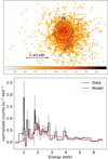 |
Fig. 1. Top: Chandra zeroth order image of the T Tau system (Ephot = 0.3–5.0 keV). North is up, east is left. Bottom: X-ray spectrum of T Tau S (zeroth order HETG, i.e., ACIS-S CCD spectrum). The red line is the 1T model. |
3.2. XMM-Newton
We use Science Analsysis System (SAS) version 13.5 with the calibration files available in Nov. 2014 and largely follow the published SAS procedures.
The Charge-Coupled Devide (CCD) spectra were extracted using standard procedures, which include the screening for periods of enhanced particle background for the spectral analysis. Light curves were corrected for detector artifacts using epiclccorr.
3.2.1. RGS spectrum
To extract spectra from the Reflection Grating Spectrometer (RGS) data, we use zeroth order positions matched to the 0.2–1.0 keV centroid. The cross-dispersion size includes 70% of the Point Spread Function (PSF). The zeroth order image of RX J0422.1+1934 is located in the RGS background region of T Tau and is therefore excluded from the background region1.
Line fluxes were measured by integration within 0.085 Å around the nominal wavelengths. This width balances between extraction efficiency and background pickup. It includes about 75–80% of the line spread function according to the instrumental response and avoids the wide instrumental line wings. For measuring line fluxes in the grating spectra, we do not subtract the background to preserve the Poisson nature of the data. Our local “background” thus includes instrumental background, weak unresolved lines, and continuum emission. We estimate this background from nearby wavelength regions without strong emission lines. As a cross-check, we compared this background estimate with the sum of the instrumental background and the flux predicted from the Astrophysical Plasma Emission Code (APEC) models fitted to the CCD spectra. We find excellent agreement between both estimates. In wavelength regions where both RGS 1 and RGS 2 have significant effective area, we average the fluxes obtained by both instruments.
The effective area varies smoothly over the wavelength regions of interest. In particular, we checked the wavelength region around the O VII triplet. There, the effective area differs only by 1% between the O VII f and i lines and by 5% between O VII r and i lines.
3.2.2. Optical monitor: UV data
During the XMM-Newton observations, the optical monitor (OM) was used with the UVW1 filter, which has a central wavelength of 2910 Å and a width of 830 Å. This filter choice allows us to compare the near ultraviolet (NUV) properties of T Tau with archival data. The OM was operated in the “Image Fast” mode so that we could generate UV light curves simultaneously to the X-ray data.
The OM detector suffers coincidence losses, which depend on the total detector count rate. T Tau provides just below 100 cts s−1, which is below the limit of several hundred cts s−1, where the SAS automatically corrects for this effect. However, count rate jumps remain between the five sub-exposures that make one full OM image. To correct this effect, we smoothly join subsequent sub-exposures while maintaining the mean count rate averaged over the observation. We convert the observed OM count rates into fluxes using the published conversion factors.
3.3. Chandra
We used the HETG for our observation, which consists of two different gratings, the high and the medium energy gratings (HEG and MEG, respectively). Each grating produces two spectral traces on the S-chips of the Advanced CCD Imaging Spectrometer (ACIS) as well as a zeroth order image with the superb angular resolution of Chandra as the HETG does not degrade the point spread function (PSF). We used the Chandra Interactive Analysis of Observations (CIAO) tools in version 4.6 (Fruscione et al. 2006) with CALDB version 4.6.3 to reduce the Chandra data.
3.3.1. Zeroth order image properties and CCD spectrum of T Tau Sab
For our analysis of T Tau N, T Tau S is a source of contaminating photons. Therefore, we estimate its properties and its contribution to the combined X-ray spectrum here. We extract individual spectra and light curves for T Tau N and S using small extraction regions centered on their nominal positions (r = 0.8 pix (≈0ʺ̣4) and r = 0.4 pix (≈0ʺ̣2) for T Tau N and S, respectively, which translates to PSF fractions of 57% (N) and 26% (S)). We experimented with different “background” regions, but found only insignificant differences. Using the contamination by T Tau N estimated from a wedge-style region (see Fig. 1 top), we found that the southern component provides 178 net counts while the northern component accumulates 1690 net counts (Ephot = 0.3–10.0 keV), which translates into a contribution fraction of 20% after correction for the different extraction efficiencies.
Using spectra binned to five counts per bin for T Tau Sab (Fig. 1, bottom) and cstatistic in xspec (Arnaud 1996), we found that an absorbed APEC2 model (Foster et al. 2012) with 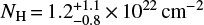 and
and  provides a reasonable fit to the data with a C-statistic of 53.0 for 38 degrees of freedom (corresponding to χred ≈ 1.2 with the caveat of non-Gaussian errors). The luminosity of T Tau Sab is log LX = 30.2 ± 0.24 (0.3–10.0 keV), which is essentially the value estimated by Güdel et al. (2007b), log LX = 30.1. Such an X-ray luminosity is somewhat higher than the typical LX of young CTTSs in the Taurus star forming region (median log LX = 29.78, see Güdel et al. 2007a), which is likely related to the high stellar mass T Tau Sa (M⋆ ≳ 2 M⊙).
Lastly, we performed a detailed spatial analysis of the zeroth order image around the northern component in a fashion similar to Schneider & Schmitt (2008) and Schneider et al. (2011) and conclude that there is no intrinsic source extension beyond a tenth of an arcsecond apart from the contamination by T Tau Sab discussed above.
3.3.2. HETG zeroth order CCD spectrum of T Tau N+Sab
We use a circular extraction region with a radius of 3″ to obtain a combined (T Tau N + Sab) spectrum for comparison with the XMM-Newton European Photon Imaging Camera (EPIC) spectra. We further bin the spectrum to a minimum of 15 counts per bin for the subsequent spectral analysis.
3.3.3. HETG grating spectra
We reduced the Chandra data with a source position derived from the photon centroid using the photons below 1 keV only to remove a possible positional shift caused by the southern component. Line counts were extracted using a 30 mÅ-wide region around the nominal wavelength of the line. This region includes about 98% of the line spread function; instrumental background is negligible. Nearby, largely line-free regions were used to estimate the continuum and unresolved line emission, and to derive line counts and fluxes.
3.4. CCD fitting procedure (EPIC and HETG zeroth order)
The combined CCD spectra (T Tau N plus T Tau Sa/Sb) are fitted with three APEC plasma emission components with variable abundances (vapec) and photo-electric absorption (phabs). In addition, we included a second component describing the emission from the southern component with the parameters (kT, NH, and EMS) fixed to the values found in Sect. 3.3.3. We also experimented with allowing a variable emission measure EMS, but found the fit to be largely insensitive to this parameter. Rather, this introduced spurious effects so that we decided to fix all parameters of the southern component during the fitting procedure.
Our detailed fitting procedure is as follows: first, we assume a single value for the absorption during all epochs and one set of temperatures for the three emission components during all epochs, while allowing the EM for each epoch and temperature component to vary freely. Since we do not have sufficiently well-exposed grating spectra for all epochs, we use three groups of abundances (elements with a low First Ionization Potential (FIP): Fe, Mg, Si, Al, Ca, Ni; mid-FIP: C, N, O, S; high-FIP: Ne, Ar). Assuming that the temperatures of the three emission components are equal in all five epochs is an unrealistic simplification, but allows us to easily investigate the evolution of the cool, intermediate, and hot components. In a second step, we release this assumption and allow the three temperatures to vary between the five epochs while still requiring the abundances and absorbing column density to be equal in all epochs (releasing the constraint on NH does not provide additional conclusive results, especially in regards to changes in absorbing column density between epochs). This approach for fitting the CCD spectra is slightly different from the method employed by Güdel et al. (2007b); in their fit to the RGS data, individual elements were allowed to vary freely. Nevertheless, the results are largely compatible.
3.5. Line fitting procedure
We obtained line fluxes by direct integration within wavelength ranges adjusted to the respective spectral resolution of the instrument (see above). To measure line ratios in the He-like triplets, we used a model with the physical quantities as fit parameters, that is, total flux and line ratios (e. g., G- and R-ratios) instead of individual line counts. Thereby, we avoid the pitfalls of propagating non-Gaussian errors and can directly obtain meaningful errors for the line ratios. This model also restricts the line ratios explored during the fitting procedure to physical ranges. We use the C-statistic (Cash 1979) for the fitting. In consequence, the line ratios (see Table 4) do not necessarily reproduce exactly the ratios resulting from dividing the counts obtained by integration of the spectra (Table 3); minor changes can be caused by the broad line wings included in the fitting procedure but neglected when integrating counts.
3.6. Ground-based data
To support the X-ray observations, we also obtained optical photometry and Hα spectroscopy.
To investigate the optical behavior of T Tau around the X-ray observations, we retrieved V band magnitudes from the American Association of Variable Star Observers (AAVSO, Henden, A.A., 2013, Observations from the AAVSO International Database3) and provide them in Fig. 2 (top). The optical brightness of T Tau is relatively constant and we estimate V = 10.3 ± 0.1 during the X-ray observations. This is about 30% dimmer than the mean observed by the Research Of Tracers Of Rotation (ROTOR) project (V ≈ 9.9 with a standard deviation of 0.1 mag, see Grankin et al. 2007).
Spectroscopic data were obtained by the Telescopio Internacional de Guanajuato Robótico Espectroscṕico (TIGRE4, Schmitt et al. 2014) and through the Astronomical Ring for Access to Spectroscopy (ARAS)5. TIGRE is a fiber-fed spectrograph in La Luz, Mexico. The fiber entrance diameter is 3″ and the spectral resolution is R ≈ 20.000; data reduction procedures are described in Mittag et al. (2010). Due to instrumental issues of the TIGRE instrument around the Chandra observation, we can only use the Hα 10% width but not the Equivilent Width (EW) for this epoch.
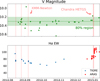 |
Fig. 2. Top: V magnitude of the T Tau system (unresolved) from AAVSO. The magnitude range containing 80% of the data is marked. The vertical lines indicate the dates of the X-ray observations. Bottom: Hα EW. |
4. Mass accretion rates
We now obtain estimates for the mass accretion rate based on established diagnostics so that we can later compare the X-ray diagnostics with these accretion tracers.
4.1. Hα line
We start our analysis with the Hα emission, one of the most widely used accretion tracers. The observed profiles are shown in Fig. 3. The overall shape of the Hα profiles remained relatively unchanged between August 2014 and January 2015. Differences in equivalent width (EW) are ≲10%, including the EW calculated from the ARAS data for the time of the Chandra observation. We provide the average values calculated for the times around the X-ray observations in Table 5, which compare well with the values observed by Costigan et al. (2014) during their 2001 observations (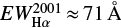 ).
).
The Hα profile appears asymmetric with more emission at negative velocities. However, decomposition into two Gaussians shows that only 15% of the Hα flux originates in a rather narrow, blue-shifted component (vpeak ≈ −70 . . . –90 km s−1, σ ≈ 40 km s−1), while the majority of the emission can be explained by a broad (100 km s−1), slightly red-shifted (v ≈ 10 km s−1) Gaussian component. The narrow, blue-shifted component is likely associated with the known jet (HH 155, e.g., Eislöffel & Mundt 1998), while the majority of the Hα emission is related to the accretion process. Therefore, it is reasonable to use the Hα luminosity to estimate the accretion luminosity despite the predominately blue-shifted velocities.
The Hα line properties have been shown to correlate with excess emission caused by accretion (UV excess or veiling; see references in Mendigutía et al. 2015). These relations typically originate from CTTS observations and have been extended to higher mass stars by simultaneously measuring accretion and line luminosities (e.g., Mendigutía et al. 2011). We provide estimates for the mass accretion below using three different diagnostics (Hα EW, Hα 10% width, NUV flux).
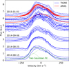 |
Fig. 3. Hα profiles (near-) simultaneous to the X-ray observations. Data from ARAS has a light copper tint and is distinguishable from the TIGRE data by its lower spectral resolution. |
4.1.1. Accretion rates from Hα equivalent width
The conversion from Hα luminosity to accretion rate is considered one of the more reliable accretion diagnostics (at least for CTTSs; see discussion in Alcalá et al. 2014). We convert the measured EW to Hα luminosity using the measured V magnitude (V ≈ 10.3; see Fig. 2 top), the average V–R from the ROTOR program (Grankin et al. 2007, V–R ≈ 1.1) and AV ≈ 1.8 (Calvet et al. 2004; Herczeg & Hillenbrand 2014). This results in a continuum surface flux near Hα of 6 × 10⁶ erg cm−2 s−1 Å−1, which corresponds well with the continuum flux published by Calvet et al. (2004), we read ≈1.5 × 10⁻¹² erg s−1 cm−2 Å−1 from their Fig. 9, while our assumed value corresponds to 2 × 10⁻¹² erg s−1 cm−2 Å−1. We are therefore confident that the error on our estimated surface flux is less than 10%. We then convert the derived Hα luminosity (log LHα/L⊙ ≈ −1) to accretion luminosity using the Calvet et al. (2004) relation and find an accretion rate of 7.8 × 10⁻⁷ M⊙ yr−1. Correcting for the outflow emission (≈15%) to the measured Hα EW and for chromospheric Hα (on the order of EW = 1 Å) lowers the accretion rate to about 6.6 × 10⁻⁷ M⊙ yr−1.
4.1.2. Accretion rates from Hα 10% width
Another measure for the accretion rate is the Hα 10% width and we find an average 10% width of 543 km s−1. Variability in the 10% width is only on the few percent level for observations falling within the XMM-Newton observing window. TIGRE data obtained with the replacement camera during the Chandra observation show, on average, a similar 10% width to the other data, but with a slightly larger scatter of 20%.
To convert the 10% width to accretion rate we use the relation presented by Calvet et al. (2004), which is based on comparing the accretion generated continuum with simultaneous Hα data for a set of intermediate-mass stars. We find that the accretion rates are mostly in the range 4–8 × 10⁻⁸ M⊙ yr−1 (only the small width observed on 2014 Sep. 6th corresponds to accretion rates <10−8 M⊙ yr−1). The average width (543 km s−1) corresponds to 2.4 × 10⁻⁸ M⊙ yr−1.
4.2. Accretion rates from NUV fluxes
We list in Table 5 the mean fluxes observed by the OM during the individual epochs. For AV = 1.8, we find emitted (dereddened) fluxes between 1.0 and 1.7 × 10⁻¹² erg s−1, which are close to the value reported by Calvet et al. (2004), FNUV ≈ 10−12 erg s−1. These authors show that most of the flux at NUV wavelengths is due to accretion. Assuming constant extinction, this indicates that changes in accretion luminosity are less than a factor of two during single exposures as well as between the four epochs. Assuming a linear relation between NUV luminosity and mass accretion rate, the UV fluxes observed by the OM indicate Ṁacc ≈ 4.4 . . . 7.5 × 10⁻⁸ M⊙ yr−1 (Calvet et al. 2004, derive Ṁacc ≈ 4.4 × 10⁻⁸ M⊙ yr−1 for FNUV ≈ 10−12 erg s−1).
4.3. Discussion of the different accretion rates
The Hα EW gives about an order of magnitude higher accretion rates than the estimates from Hα 10% width and NUV fluxes. Since our value from the EW is similar to previous estimates also based on EW (Costigan et al. 2014, Ṁacc = 1.4 × 10⁻⁶ M⊙ yr−1), we consider the discrepancy as inherent to the employed method. The Hα EW, while qualitatively correlating well with accretion, also shows a large scatter with respect to other tracers. Since 10% width as well as NUV excess, which directly traces the accretion shock emission, suggest similar rates, we assume in the following Ṁacc = 5 × 10⁻⁸ M⊙ yr−1 as representative. This value is rather typical for (high-mass) CTTSs (Calvet et al. 2004). In addition, the observed trend between stellar mass and accretion rate with Ṁacc ∝ M2.1 implies Ṁacc = 7 × 10⁻⁸ M⊙ yr−1 for T Tau (see Hartmann et al. 2016), which is very close to the derived values given the observed scatter. In summary, T Tau’s mass accretion rate and its minor variability are rather typical for stars of its mass and age (Venuti et al. 2014).
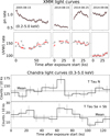 |
Fig. 4. Top: XMM-Newton X-ray and UV light curves. For the OM, the gray data points indicate the pipeline values before correcting for variable coincidence losses (for details, see Sect. 3.2.2). Bottom: Chandra X-ray light curves. |
Using Eq. (1) from Güdel et al. (2007b), we use our estimate for the mass accretion rate to estimate the post-shock density of an homogeneous accretion spot covering 10% of the stellar surface (i.e., surface covering fraction 0.1) and find ne = 2 × 1012 cm−3, which is in the sensitivity range of the X-ray density diagnostics with the O VII and Ne IX He-like triplets.
5. General plasma properties from X-ray CCD spectra
We start our investigation of the X-ray properties of T Tau with the light curves before moving to the plasma properties derived from CCD spectroscopy.
Light curves and spectra
The X-ray light curves (Fig. 4) reveal almost a factor of two difference between the epochs, but no obvious flares, and we use a single spectral model for each epoch; only the 2005 epoch shows some variability, but we decided to fit a single model to preserve comparability with the results presented by Güdel et al. (2007b).
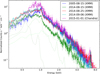 |
Fig. 5. CCD X-ray spectra of T Tau. The extraction region encompasses T Tau N and S to enable a direct comparison of the spectra. XMM-Newton EPIC spectra have been merged for this plot. For illustration purposes, the dotted green lines indicate the contributions of the individual plasma components for the 2014 Aug. 15th epoch. |
CCD spectral fits with 90% confidence ranges.
Figure 5 shows the CCD spectra. Differences are more pronounced in the soft band (Ephot ≤ 1.0 keV) than in the hard spectral range (Ephot > 1 keV), where four out of five epochs show similar fluxes. The lowest fluxes are observed for the 2014 Aug. 15th epoch by a factor of two. Ten days later, the fluxes are back to the “normal” level.
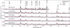 |
Fig. 6. Atlas of X-ray grating spectra. “Mean” indicates the mean observed spectrum. |
We experimented with several fit approaches, for example, a single temperature grid for all epochs or variable temperatures. We found that the fit results obtained with a single temperature grid for all epochs already provides a decent description of the data (χred ≈ 1.11) while more complex models only mildly improve the fit (χred ≈ 1.08). Therefore, we provide these values in Table 2 to ease inter-comparison between the epochs. Differences between the various fit approaches are mainly in the EM of the individual components, while temperatures and abundances remain relatively stable, for example, temperature changes are mainly in the 10–30% range. Specifically, the coolest component’s temperature is stable (we find Tcool = 1.7 × 10⁶ K with typical errors of 0.1–0.2 × 10⁶ K, i.e., slightly lower than the 1.9 × 10⁶ K obtained from the joint fit). Notable is the low EM1 for 2005 Aug. 15th in the fit using a single temperature grid that is not mirrored by a particularly weak O VII emission in the corresponding RGS spectrum. Closer inspection shows that the particularly low EM1 in Table 2 for 2005 Aug. 15th is partly based on a true lack of soft emission (about a factor of two lower than in the brighter epochs, cf. Fig. 5), but mainly due to the cross-talk between the lowest and the intermediate temperature components: the intermediate temperature component is responsible for most of the flux at low energies and there is little space for emission from the low temperature component except for isolated lines like O VII. Allowing the fit to vary the temperatures freely between the epochs changes EM1/EM2 from 1:13 to 1:2, which is more in line with the RGS spectrum where strong O VII emission is seen. The low EM3 for 2014 Aug. 15th, however, is clearly visible in the CCD spectra where the lowest fluxes are observed above Ephot ≈ 0.6 keV and remains essentially unchanged in the free temperature fit. Inspection of the Fe complex around Ephot ∼ 6.7 keV further suggests a higher Fe abundance of the hottest plasma component during all epochs, and weak Fe Kα emission in one epoch.
The expected post-shock plasma temperature is below 5 MK for the free fall velocities >600 km s−1, the maximum amenable for T Tau N (see Table 6). Therefore, the two hotter temperature components must be associated with coronal emission and are responsible for 70–80% of the total X-ray flux (0.3–10.0 keV, depending on epoch). They indicate magnetic activity as expected given the measured ∼kG magnetic field (Johns-Krull 2007). Thus, the X-ray spectrum of T Tau above 0.5 keV appears similar to low-mass CTTSs and differs from young but magnetically inactive A type stars of similar stellar mass like β Pic, which generate orders of magnitude weaker X-ray emission (Günther et al. 2012).
The cool plasma component T1 has a typical luminosity of about 2.6 × 1030 erg s−1 and dominates the observed emission only at photon energies around O VII (Ephot ≈ 0.6 keV) and below during some epochs (see Fig. 5). It dominates the O VII emission by at least one order of magnitude while the Ne IX emission (Ephot ≈ 0.9 keV) originates in both the cool and the intermediate temperature components (ratio about 1:2).
In summary, the CCD spectra indicate plasma properties similar to those found in active, accreting stars (cf. the XEST results, Güdel et al. 2007a). The observed X-ray fluxes (6–10 × 1030 erg s−1 for the 0.3–10.0 keV band) correspond to log LX/L⋆ = −3.5 (for L⋆ = 7.5 L⊙, see White & Ghez 2001), typical for very active stars (Brickhouse et al. 2010; Robrade & Schmitt 2007; Günther et al. 2007; Telleschi et al. 2007a) and published relations between stellar mass and X-ray luminosity (Telleschi et al. 2007a) suggest log LX ≈ 30.88, which is within a factor of two of the measured values.
Also, the abundance pattern known as the inverse first ionization potential effect (iFIP) and the variability (factor two, no flares) are similar to previous X-ray observations of accreting intermediate-mass stars. In summary, the X-ray properties from CCD spectroscopy of T Tau are similar to those observed for other (massive) CTTSs.
Observed line fluxes in units of 10−6 counts s−1 cm−2.
6. Line ratios from grating spectra
Figure 6 shows the RGS and HETG grating spectra. We concentrate on a number of interesting diagnostic lines, but do not perform a detailed spectral modeling. Our observing strategy with multiple shorter exposures results in a comparably low number of reliably measurable lines so that we prefer to obtain plasma properties and absorbing column density from the CCD spectra. Important line fluxes are provided in Table 3. Because these lines are at quite low energies (Ephot < 0.9 keV), contamination by T Tau S is negligible.
In the following, we focus on He-like triplets. The terms r, i, and f indicate the resonance, intercombination, and forbidden lines. Their line ratios depend on temperature (G-ratio: (f + i)/r) and on a combination of density and local UV field (R-ratio: f/i). Higher densities as well as high UV fluxes decrease the R-ratio, that is, larger ratios correspond to lower densities and low UV fluxes. In CTTSs, the photospheric UV field is considered too weak to significantly affect the R-ratio, and high density measurements have been regularly interpreted as high plasma densities (e.g., Telleschi et al. 2007a).
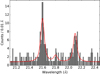 |
Fig. 7. Merged RGS spectra around the O VII triplet. |
6.1. Oxygen
The oxygen lines provide us with important information on the lowest temperature plasma possibly emitted by the immediate post-shock plasma. They are measured from the XMM-Newton RGS spectra since too few photons were recorded in this region in the Chandra HETG observation.
In principle, the G-ratio provides us with information on the temperature of the O VII emitting plasma. The measured values (between 0.6 and 1.2) indicate temperatures in the range between log T = 6.0 . . . 6.7, however, the 90% credibility ranges extend from log T < 6.0 to log T > 7.0. Therefore, we use T1 from the CCD spectroscopy, which is close to the peak formation temperature (log T = 6.3). The predicted line fluxes are in good agreement with the measured values (using the CHIANTI database, see Young & Landi 2009). Hence, we consider T1 as a good estimate of the O VII emitting plasma fully consistent with the measured G-ratios.
Line ratios. Values in brackets are 1 σ confidence ranges.
6.1.1. R-ratio: Density of the O VII-emitting plasma
Figure 7 shows that the forbidden line is stronger than the intercombination line during all epochs. The detailed results from line fitting listed in Table 4 reveal that the lower limit on the f/i-ratio is about two while the formal upper limit corresponds to the theoretical limit. The 90% confidence limits are log ne < 10.5 . . . 10.9 for the individual epochs, which is similar to the upper limit found by Güdel et al. (2007b) for the 2005 observation. This demonstrates that the densities during the 2005 XMM-Newton observation are rather typical for T Tau.
Coadding the four epochs of RGS data results in log ne < 10.0 and <10.4 for the 1 σ and 90% confidence ranges, respectively. The corresponding densities depend slightly on the plasma temperature and we have assumed a temperature of log T = 6.3 for the above estimates (about T1 from our CCD fits and compatible with the G-ratio). Varying the plasma temperature by ± 0.2 dex changes these limits by less than 0.1 dex while simultaneously reducing the O VII emissivity by a factor of two. The upper limit is lower than the density estimated in Sect. 4.3, and it is even lower than the post-shock density of an accretion funnel carrying the derived accretion rate and covering the entire stellar surface (such an artificial shock would have ne = 2 × 1011 cm−3). Therefore, other processes must be invoked to explain the O VII emission.
6.1.2. Soft excess
The soft excess is defined as the dereddened ratio between the O VII r and O VIII Ly α line fluxes (Güdel & Telleschi 2007; Robrade & Schmitt 2007). It depends on the assumed absorbing column density. In Appendix A, we show that, in contrast to TW Hya, we do not find a different absorption towards the O VII emitting region and towards the corona. Therefore, we use NH = 3 × 1021 cm−2 as derived from the CCD spectroscopy.
Figure 8 shows the soft excess for each epoch in comparison with other stars. T Tau’s soft excess is statistically equal in all epochs, and greatly surpasses the excess seen in other young stars.
6.2. Neon
The Ne IX triplet (with wavelengths of 13.45, 13.55, and 13.70 Å for the recombination, intercombination, and forbbiden lines, respectively) can trace the density of plasma emitted at higher temperatures than O VII (approximately 4 versus 2 MK), though with the caveat of a higher coronal contribution than in O VII. The spectral resolution of the RGS is insufficient to reliably resolve the triplet components from the “contamination” by nearby Fe lines so that we concentrate on the HETG.
Close inspection of the two MEG gratings orders reveals that only two photons are detected in the f + i lines of the negative grating order, which is statistically quite unlikely given the number of r-line photons (11) and the photon number detected in the positive grating order at similar effective area (11 in the f + i lines). This discrepancy might be related to an unknown (perhaps localized) detector artifact not fully accounted for by the reduction software, possibly caused by the proximity of the f-line (and to a lesser degree of the i-line) to the chip gap in the negative grating order although our data are insufficient to demonstrate this conclusively. We focus on the positive grating order in the following, but also provide the results for the combined data for comparison in square brackets. Due to the low number of counts, the confidence ranges usually overlap making this decision less critical for the physical interpretation.
 |
Fig. 8. Soft excess of T Tau compared with other T Tauri stars as well as main sequence stars. Main sequence stars are mainly from Ness et al. (2002, 2004). The decrease of the O VII to O VIII ratio with increasing oxygen luminosity is a result of the increasing average coronal temperature for increasingly active MS stars (e.g., Johnstone & Güdel 2015). Plot symbol sizes scale with mass accretion rate. |
The G-ratio above 0.8 [0.6] indicates a plasma temperature below 4.4 × 10⁶ K [6.3 × 10⁶ K]. This points to an origin in the low-temperature plasma component – similar to the oxygen VII triplet. The R-ratio above 2.5 [1.2] indicates densities below log ne = 11.4 [12.1]. Factoring in the coronal contribution, the limits are 11.9 [13.3]. In summary, the data indicate that the Ne IX emission originates in a rather cool (a few MK), low density plasma, although the formal 90% confidence limit using both grating orders is not very restrictive.
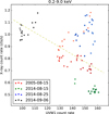 |
Fig. 9. X-ray count rates (pn) compared to OM UVW1 count rates with colors indicating the individual epochs. OM data are averages within the respective 2 ks pn light curve bins. |
Exposure averaged UV count rates and fluxes, and mean contemporaneous Hα properties.
7. X-ray versus NUV emission
Previous studies provided evidence for a negative correlation between X-ray luminosity and accretion rate in different samples of stars and non-simultaneous data (e.g., Telleschi et al. 2007a). We use the T Tau data to check this correlation on a single star using pn and UVW1 count rates as tracers of X-ray luminosity and accretion rate (the UVW1 band is dominated by accretion shock emission; see Calvet et al. 2004). Stellar activity contributes to both wavelength regimes, which likely weakens any signal from correlated accretion-X-ray variability. However, only two short events show correlated X-ray-UV variability that might be related to flares so that most of the variability must have a different origin.
Figure 9 shows the correlation between X-ray emission and NUV count rate. There is a tendency for the X-ray count rate to decrease with increasing NUV flux. Taking the XMM-Newton energy band (0.2–9.0 keV), we find a significant negative correlation (–0.39 with a p value of 10−4 for Spearman’s R; similar results are obtained for Kendall’s τ and Pearson R). We examined individual energy bands and find that the correlation is driven by the energy band providing the largest count numbers while there is no significant change of the spectral hardness as a function of UV count rate. It is noticeable, however, that the soft band (Ephot < 0.6 keV) shows no significant correlation with UV count rate.
At first sight, the correlation appears to be driven by the 2014 Sep. 6th observation. Omitting this particular epoch still results in negative albeit less significant correlations. On the other hand, only some epochs show negative correlations while others show positive correlations. Therefore, the overall anti-correlation only applies on average, but not on short timescales.
To compare our results with published relations, which are typically expressed as power laws (log LX = a + b log Ṁ), we approximate the conversion from count rates to X-ray/accretion luminosities by first order polynomials (e.g., accurate to within 6% for X-ray luminosities) and ignore any photospheric contribution to the UVW1 flux (accurate to about 10%).
With these transformations, we find that the X-ray luminosity scales as log LX ∼ – (0.74 ± 0.13) log Ṁacc, where we considered the error in accretion and X-ray luminosity using total least squares. Specifically, to compare our results with Telleschi et al. (2007a), we consider the so-called residual X-ray luminosity, that is, we divide the X-ray luminosity by the expected X-ray luminosity based on stellar mass6 (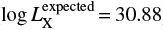 ) and find
  with an unconstrained lower bound for the constant term due to the interplay with the linear term. This relation is compatible with the Telleschi et al. (2007a) power law found for a sample of stars with non-simultaneous accretion rate measurements (log LX/L(Ṁ) = −(4.05 ± 1.19) ȡ (0.45 ± 0.15) log Ṁacc). Therefore, the residual X-ray luminosity of T Tau varies with accretion rate in the same sense as observed for samples of T Tauri stars.
Comparison of T Tau with some other CTTSs and HAe stars that have high-resolution X-ray grating spectroscopy.
8. Discussion
8.1. Comparison of T Tau’s X-ray grating spectroscopy to other CTTSs and HAe stars
We first concentrate on the line diagnostics from our X-ray grating spectroscopy. The O VII (and to a lesser degree the Ne IX) line ratios differentiate T Tau from other, lower mass CTTSs, which generally show high densities in the O VII and Ne IX triplets. In particular, we measure an O VII R-ratio of ≳2 for T Tau, while other single CTTSs have R-ratios between 0.2 and 0.4; for example 0.21 ± 0.07 (TW Hya, Brickhouse et al. 2010), 0.3 ± 0.2 (RU Lup, Robrade & Schmitt 2007), 0.37 ± 0.16 (BP Tau, Schmitt et al. 2005), or 0.28 ± 0.13 (MP Mus, Argiroffi et al. 2007). A similar pattern is found in Ne IX, where our lower limit is below the value derived for TW Hya (>2.5 in T Tau versus 0.51 ± 0.03 in TW Hya, Brickhouse et al. 2010).
T Tau’s oxygen and neon R-ratios are more comparable to those found in HAe stars, where X-ray grating spectra mostly indicate low densities (e.g., AB Aur, HD 163296, see Telleschi et al. 2007b; Günther & Schmitt 2009, resp.). We will therefore use these as representative for HAe X-ray data in the following. The HETG spectrum of the Herbig Ae star HD 104237 shows densities around 1012 cm−3 (Testa et al. 2008) and does not fit this pattern. However, HD 104237 is a spectroscopic binary, which makes conclusions based on this measurement less robust than for the two bona fide single HAe stars.
The similarity of T Tau with HAe stars in terms of X-ray density diagnostics suggests that the mass accretion rate, which T Tau shares with HAe stars (e.g., 10−7 M⊙ yr−1 for HD 163296 while TW Hya has only a few 10−9 M⊙ yr−1), is more important than the magnetic field strength, which T Tau shares with CTTSs but not with HAe stars (e.g., the upper limit for HD 163296 is about 50 G; see Hubrig et al. 2007). Therefore, we concentrate on the properties of the accretion shock to explain the differences between T Tau, CTTSs, and HAeBe stars, and ignore, for the moment, the effect of the magnetic field, which is clearly a strong simplification. In fact, there is evidence from Zeeman-Doppler Imaging that magnetic fields on higher-mass CTTSs are likely more complex than on their lower-mass siblings, which have predominately dipolar magnetic fields (Gregory et al. 2012). This probably also influences the accretion process and causes higher accretion shock densities for magnetic fields dominated by higher multipole moments (Adams & Gregory 2012). Nevertheless, we argue that the shock itself remains largely unaffected as long as the magnetic field strength is sufficient to channel the material onto the stellar surface. Furthermore, the similarity in the X-ray-derived densities between T Tau and, for example, the HAe star HD 163296, despite their strongly contrasting magnetic field configuration, argues against a decisive impact of the magnetic field on the observed X-ray emission from the accretion shock.
8.2. The origin of the O VII emission and the soft excess
We now argue that the O VII emitting plasma cannot be associated with direct post-shock emission. We specifically consider three example cases: one representative of the well-studied low-mass, magnetic CTTS (TW Hya); one representative of the non-magnetic HAe stars (HD 163296); and, T Tau as being squarely intermediate between these two examples. Their general properties as well as those for other young, accreting stars with X-ray grating spectroscopy are summarized in Table 6.
The accretion rates derived based on X-ray fluxes generally tend to fall short of those from more traditional accretion tracers (e.g., from optical emission lines fluxes, see Curran et al. 2011). In particular, the O VII density diagnostics show that the plasma cannot carry the bulk of the accretion rate, simply because the total accretion rate would be too low for T Tau (see Sect. 6.1.1) and HD 163296 (see Günther & Schmitt 2009). A comparable argument applies to TW Hya: Brickhouse et al. (2010) locate the O VII emitting plasma in the low-density “splatter”, because it is, first, subject to a lower absorbing column density than the Ne IX emitting plasma (which is likely associated with the accretion shock) and, second, has a lower density than the Ne IX emitting plasma, which is opposite to expectations from shock models. In other words, the mass-accretion rates associated with the O VII emitting plasma fall short of the rates derived from other accretion tracers by almost one (TW Hya) to several orders of magnitude (T Tau and HD 163296), when using literature values for the accretion spot sizes, the constraints on the plasma density, and reasonable values for the infall velocity (see references provided in Table 7).
Physical parameters used.
In addition, requiring that the O VII emitting plasma has a similar spatial footpoint to the accretion spot(s) provides an insufficient amount of post-shock emission measure (EM) for T Tau and HD 163296 (see Table 7). Specifically, we approximate the radiative cooling length as
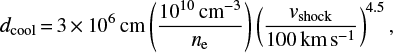 (1)
(1)
derived from Fig. 5 in Günther et al. (2007), with the infall (or shock) velocity vshock and the pre-shock electron density ne, which is related to the measured (= post-shock) density via ne = nmeasured/4. The upper limit7 for the emission measure of the post-shock plasma is then
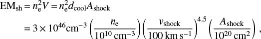
where Ashock is the surface area of the shock and we use the O VII measured densities for the post-shock density. We further use the EM of the coolest plasma component, in which the vast majority of the O VII emission originates, factoring out differences in oxygen abundance8 to avoid biasing this comparison. With this approach, we ignore any contribution from the corona to the soft plasma component. In fact, the soft excess tells us that the corona most likely contributes only a little (20–30%) to the soft plasma component assuming that coronae on CTTSs are scaled-up versions of main-sequence star coronae. Clearly, the O VII emission in T Tau and HD 163296 originates in a structure, which has a larger vertical height than the cooling distance while this is not necessary for TW Hya although a more detailed treatment will likely reveal that the emissivity of the post-shock plasma is insufficient for the observed emission measure even in TW Hya. This is in line with Brickhouse et al. (2010) who “arbitrarily” increase the vertical scale height of the cool plasma to 0.1 R⋆ in order to produce the required emission measure.
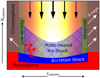 |
Fig. 10. Not-to-scale sketch of the envisaged accretion shock geometry. The observed X-rays originate in the outer shell of the accretion stream, which carries only a small fraction of the total accretion rate. |
In summary, we find that (a) only a small fraction of the O VII emission can be potentially associated with post-shock cooling plasma and (b) the O VII emission can only represent a small fraction of the accretion luminosity. Therefore, we need a mechanism that increases the scale height of the cool plasma while simultaneously blocking most of the direct post-shock emission.
8.3. Photo-heated, density stratified accretion columns
We propose radially density stratified accretion columns (see sketch in Fig. 10). This model is based on the global Magneto-Hydrodynamic (MHD) models of Romanova et al. (2004) and includes the radiation transport studied by Costa et al. (2017). First, the MHD models show that accretion columns have a dense inner core surrounded by lower density material, while, second, the radiation from the hot post-shock plasma heats the pre-shock material and increases the scale height of the hot plasma. We envision the density profile of the stream to increase radially from the outside to inside, which determines the optical depth to each point of the X-ray emitting post-shock plasma and, thus, also the mean density of the plasma observed at X-ray wavelengths and the fraction of the energy released in the shock that escapes at X-ray wavelengths.
The radial density stratification results, first, in a dense inner core of the accretion stream that provides the bulk of the accretion material, but is largely invisible in X-rays due to absorption by the incoming (pre-shock) gas and, second, increases the vertical height of the hot plasma since the post-shock emission is not only absorbed by the pre-shock material at the same streamline (as in the model by Costa et al. 2017) but also cannot escape unhindered radially as the aspect-ratio (height/radius) is around unity for T Tau and HD 163296 (2.4 and 0.2, respectively). For TW Hya, the aspect ratio is 0.01 implying that the post-shock radiation can escape more easily in the vertical direction assuming some moderate tilt in the accretion column. The observed O VII emission does not come entirely from the post-shock plasma. In our scenario, the pre-shock plasma contributes, too. The high-energy photons from the inner, high-density regions of the accretion shock are mostly re-processed in the pre-shock material, both on the same and on other streamlines. These photons heat and ionize part of the infalling material before it goes through the terminal shock at the stellar surface. Photons from the low-density, outer parts of the accretion stream dominate the emission from the pre-heated material, because these regions suffer less extinction toward the observer and have longer equilibrium timescales than the dense, inner accretion stream regions. Re-processing only a small fraction of the energy released in the accretion-shock into O VII emission is sufficient to cause the soft excess. In addition to the high-energy post-shock photons, a reverse shock may also contribute to the pre-heating of the accretion funnels (see laboratory experiments by Revet et al. 2017). In reality, some combination of these two processes is likely responsible for the O VII emitting plasma in the low-density regions of (or around, Orlando et al. 2013) the accretion funnel above the stellar surface since other mechanisms are thought to be insufficient (such as thermal conduction, see Orlando et al. 2010; Revet et al. 2017). In order to thoroughly test this scenario, one needs detailed MHD-radiation transfer calculations, which are beyond the scope of this paper. Also, the above scenario of radially stratified accretion columns does not exclude other contributions to the soft excess such as a splatter or a reverse shock in the case of high-β conditions9 in the post-shock region (Brickhouse et al. 2010; Revet et al. 2017).
Stars like TW Hya with a low accretion rate also have a low pre-shock column density that absorbs a comparably small fraction of the immediate X-ray emission from the accretion shock and the observed emission is dominated by the dense inner part of the accretion stream. With increasing mass accretion rate (T Tau and HD 163296), a larger fraction of the post-shock emission must pass through large columns. Thus, this emission does not escape, but heats the pre-shock plasma above the accretion shock. This increases the aspect ratio and decreases the observed density as only the emission originating in the outer, low density shells can escape relatively unhindered.
For a fiducial area of the dense, inner stream of one tenth of the outer, low density part, that is, covering fractions of 0.3%, 0.3%, and 0.8% for T Tau, TW Hya, and HD 163296, respectively, we find that densities of log n = 13.5, 13.1, 13.8 for T Tau, TW Hya, and HD 163296, respectively are required in the inner stream to carry the accretion rates derived from established accretion diagnostics (e.g., UV excess). These high densities result, first, in rather short cooling distances so that the radius of the stream largely exceeds the shock cooling distance (cf. Fig. 10). Second, this inner, high density shock results in large emission measures associated with the core of the accretion stream. The emission measures associated with the post-shock cooling zone of the inner funnel would outshine the outer, low density part of the accretion stream (and the corona) without absorption for T Tau and HD 163296 (EM > 1054 cm−3). The emission from this dense plasma is, however, absorbed in the pre-shock plasma. For example, 10% of the inner, dense column in the radial direction already corresponds to a column density of >2 × 1022 cm−2, which extinguishes the O VII and Ne IX triplets in T Tau and HD 163296. Since the fraction of the soft X-ray to accretion emission is largest in TW Hya, the emission measure associated with the inner part of the accretion spot is comparable to the one observed (EM = 7 × 1052 cm−3) as expected. While the innermost part of the stream remains obscured, the emission from the slightly less dense surrounding shells can escape, thus explaining the high densities.
The densities of the inner stream that we derive here exceed the typically quoted values (∼1013 cm−3, see review by Hartmann et al. 2016). These densities are derived from traditional accretion tracers such as UV excess assuming a homogeneous density in the accretion stream. However, the average density of the radially density stratified accretion stream is lower than the values for the inner stream so that the densities in our scenario compare quite well with the literature values.
The deep X-ray grating spectrum of TW Hya allows us to perform an additional test of our scenario. The excess absorption provided by the O VII emitting region, that is, the “splatter” in the Brickhouse et al. (2010) model, is the low density outer stream in our model. The absorbing column density towards the O VII emitting region is 2 × 1020 cm−2 while the column density towards the Ne IX emitting region is 2 × 1021 cm−2. Assuming a linear increase in density from the O VII emitting region (ne = 6 × 1011 cm−3) to the Ne IX emitting region (ne = 3 × 1012 cm−3), the required distance to accumulate an absorbing column density of 1.8 × 1021 cm−2 is 109 cm, which is about the value estimated by Brickhouse et al. (2012) for a constant density. Given the simplicity of this model, this value is surprisingly close to the sizes estimated above for the inner, high density part of the accretion stream in TW Hya (2 × 109 cm).
This scenario also mimics individual aspects of models already proposed in the literature. From an X-ray point of view, it includes the absorption effects proposed by Brickhouse et al. (2010) as the outer layer of the accretion stream has a similar role as the “splatter” in the Brickhouse et al. (2010) model, that is, it is responsible for the softest X-ray photons while also absorbing the central region of the accretion shock. It includes the optical depth effects discussed by Sacco et al. (2010) and Curran et al. (2011) as the cause of the low-mass accretion rates derived from X-ray (O VII) line fluxes. In our model, however, the observed X-ray emission is not caused by “appropriate” streams, but rather by the “appropriate” outer shells of the stream. Also, our model includes optical depths effects already discussed by Argiroffi et al. (2009), mainly for resonance line scattering, which would massively affect the G-ratio for which we do not find any hint in our data; the observed G-ratio is fully compatible with those expected for a thermal plasma emitting O VII photons and in more detail by Bonito et al. (2014).
8.4. Accretion versus X-ray emission
Analysing the EPIC pn and OM data, we find that higher UV fluxes correspond, on average, to lower X-ray luminosities. We interpret this as an anti-correlation between accretion and (magnetic) X-ray activity, because the majority of the observed X-ray and UV variability is rather smooth and happens on timescales comparable to the duration of the observations (half a day and longer). Flaring activity could affect this relation, but only two short-duration, weak events are present so that we regard stellar activity as unlikely to dominate over accretion effects in our data. Similarly, time lags between accretion-driven UV excess and X-ray response (e.g., Dupree et al. 2012) or vice versa might weaken the correlation but are not expected to spoil the correlation given the smooth variations (we also checked that reasonable time lags do not improve the correlation).
Our analysis of the accretion-X-ray luminosity correlation is complementary to published studies, which rely on (mostly) non-simultaneous data for different samples of stars (e.g., Neuhäuser et al. 1995; Preibisch et al. 2005; Telleschi et al. 2007a; Güdel et al. 2007b; Bustamante et al. 2016) while we investigate the correlation between accretion and X-ray luminosity for a single star. Interestingly, our correlation is compatible with published studies, for example, Telleschi et al. (2007a) for the XMM-Newton Extended Survey of Taurus (XEST) sample (Güdel et al. 2007a) and Bustamante et al. (2016) who estimate accretion rates based on U-band excess for Orion Nebular Cloud (ONC) stars, a method that is similar to our UV excess approach.
Given that the correlation between accretion rate and X-ray luminosity observed for samples of stars extends to different accretion rates for an individual star, we shall interpret these correlations either in terms of accretion suppressing (detectable) X-ray emission (a causal effect) or in terms of a third property that influences both X-ray emission and accretion. Other phenomena, for example, stellar evolution, can be excluded.
On an individual star, accretion variability on day to week timescales is thought to be mainly due to rotational modulation; only rare accretion bursts occasionally enhance the accretion rate (e.g., Costigan et al. 2012, 2014; Venuti et al. 2014; Rigon et al. 2017). Following this reasoning, the variability in the accretion rate as traced by the NUV flux is driven by T Tau’s rotation. The anti-correlation between accretion rate and X-ray flux then implies that rotation also is responsible for part of the X-ray variability (Güdel et al. 2007b, already suggest that some of the X-ray variability is due to rotation). This might be explained by the ratio between closed and open field lines. The open field lines connect the star with the disk and carry the accretion material. For the Sun, we know that the X-ray emission originates in closed loops while open field lines contain thin plasma producing little X-ray emission. Therefore, the hemisphere covered with a larger fraction of open field lines shows stronger accretion signatures and emits less X-ray emission.
This would fit into our scenario of density stratified accretion columns. The thin, outermost regions of the stream are unlikely to be visible in the X-ray regime or in other tracers, because of their low density, but might still interfere with coronal structures thus reducing the harder X-ray emission. This requires a very low density layer around the funnels, which covers a relatively large fraction of the star (a few 10%). This layer would not cause other observable features due to its low density; especially the photosphere would remain largely unaffected by the impact of very low density material. Also, virtually no extinction would be associated with the low density outermost shells of the accretion stream (for a fiducial value of n = 109 cm−3, the absorbing column density for a length corresponding to the stellar radius would be in the 1020 cm−2 range, which is low compared to the measured NH values).
9. Summary and conclusions
We have analyzed four new X-ray observations of T Tau and accompanying NUV data, Hα profiles, and optical photometry. Our main observational results can be summarized as follows:
The strong X-ray soft excess is present in all four XMM-Newton observations spanning timescales from weeks to years.
The O VII triplet is compatible with the low density limit in all four epochs. This demonstrates that this feature is stable and that variability in T Tau’s accretion properties cannot explain the difference to its lower mass siblings.
Similar to the O VII triplet, the Ne IX triplet shows low densities. This suggests that the emission from plasma with temperatures of a few MK is dominated by low density material.
Accretion rates between 4 and 8 × 10⁻⁸ M⊙ yr−1 apply for the times of the X-ray observations.
There is about a factor of two variability during and between the exposures in all fluxes (soft, X-rays, hard X-rays, and NUV photometry). Most of the variability happens smoothly on timescales comparable to the on target times. A few short, isolated events exist but do not dominate the variability.
X-ray and NUV variability is anti-correlated. This anti-correlation mirrors the anti-correlation between X-ray luminosity and accretion found in samples of CTTSs.
We further discussed the low density finding and the soft excess in terms of radially stratified accretion columns and the X-ray-NUV flux anti-correlation in terms of magnetic field effects.
First, density stratified accretion funnels provide a natural explanation of the X-ray diagnostics of CTTSs by merging features of existing models: accretion generated X-ray emission is only seen from the outer, low density radii of the accretion funnel while the inner, high density part of the stream is obscured from view but carries the majority of the accretion. In this scenario, the origin of the soft excess is similar in all accreting stars while the difference in density diagnostics between low- and intermediate-mass stars is ascribed to different escape probabilities between the dense inner and thin outer parts of the accretion streams. Higher accretion rates with more important higher magnetic multipole moments in intermediate-mass stars result in lower observed densities than the lower accretion rates and more important dipole components in lower-mass stars.
Second, the anti-correlation between X-ray flux and accretion rate found for T Tau extends similar relations for samples of stars, which strongly suggests that this anti-correlation is driven by a phenomenon intrinsic to processes on accreting stars. We suggest that the stellar magnetic field plays a key role through enhancing X-ray emission in surface patches with closed magnetic field lines while simultaneously enhancing accretion signatures in patches with large fractions of open field lines.
In the future, a more systematic study of the transition region between high and low density X-ray diagnostics in CTTSs and HAe stars can help to confirm the proposed model of density stratified accretion funnels, which would be ideally supplemented by magnetic field studies on the very same stars. In addition, the XMM-Newton archive contains numerous observations of CTTSs during which the OM was operated with UV filters that include accretion driven emission. Hence, extending our correlation analysis between UV and X-ray count rates can extend the short term correlation between accretion rate and X-ray luminosity on individual stars. A broader data coverage would solidify the accretion-X-ray anti-correlation.
Acknowledgments
PCS gratefully acknowledges support by DLR 50 OR 1307 and an ESA Research Fellowship during which part of the analysis was conducted. HMG acknowledges support by NASA-HST-GO-12315.01. The results reported in this article are based on observations made by the Chandra X-ray and the XMM-Newton Observatories. This work also made use of data from the European Space Agency (ESA) mission Gaia (https://www.cosmos.esa.int/gaia), processed by the Gaia Data Processing and Analysis Consortium (DPAC, https://www.cosmos.esa.int/web/gaia/dpac/consortium). Funding for the DPAC has been provided by national institutions, in particular the institutions participating in the Gaia Multilateral Agreement. Support for this work was provided by the National Aeronautics and Space Administration through Chandra Award Number GO5-16014X issued by the Chandra X-ray Observatory Center, which is operated by the Smithsonian Astrophysical Observatory for and on behalf of the National Aeronautics Space Administration under contract NAS8-03060.
This expected X-ray luminosity can be based on stellar mass or on the relation between stellar mass and mass accretion rate, log Ṁ = 2 log M – 7.5.
This simplified treatment assumes constant, high temperature within dcool while the temperature gradually decreases with increasing distance from the shock location in reality.
We multiply EM with the oxygen abundance relative to T Tau since the absolute metallicity is not well defined. Therefore, we consider these values more suitable for this comparison, but note that our conclusions are qualitatively insensitive to these details.
The value β describes the ratio between plasma and magnetic pressure.
References
- Adams, F. C., & Gregory, S. G. 2012, ApJ, 744, 55 [NASA ADS] [CrossRef] [Google Scholar]
- Akeson, R. L., Koerner, D. W., & Jensen, E. L. N. 1998, ApJ, 505, 358 [NASA ADS] [CrossRef] [Google Scholar]
- Alcalá, J. M., Natta, A., Manara, C. F., et al. 2014, A&A, 561, A2 [NASA ADS] [CrossRef] [EDP Sciences] [Google Scholar]
- Alecian, E., Wade, G. A., Catala, C., et al. 2013, MNRAS, 429, 1001 [NASA ADS] [CrossRef] [Google Scholar]
- Anders, E., & Grevesse, N. 1989, Geochim. Cosmochim. Acta, 53, 197 [Google Scholar]
- Argiroffi, C., Maggio, A., & Peres, G. 2007, A&A, 465, L5 [NASA ADS] [CrossRef] [EDP Sciences] [Google Scholar]
- Argiroffi, C., Maggio, A., Peres, G., et al. 2009, A&A, 507, 939 [NASA ADS] [CrossRef] [EDP Sciences] [Google Scholar]
- Arnaud, K. A. 1996, ASP Conf. Ser., 101, 17 [Google Scholar]
- Batalha, C. C., Quast, G. R., Torres, C. A. O., et al. 1998, A&AS, 128, 561 [NASA ADS] [CrossRef] [EDP Sciences] [Google Scholar]
- Batalha, C., Batalha, N. M., Alencar, S. H. P., Lopes, D. F., & Duarte, E. S. 2002, ApJ, 580, 343 [NASA ADS] [CrossRef] [Google Scholar]
- Bonito, R., Orlando, S., Argiroffi, C., et al. 2014, ApJ, 795, L34 [Google Scholar]
- Bouvier, J., Covino, E., Kovo, O., et al. 1995, A&A, 299, 89 [NASA ADS] [Google Scholar]
- Brickhouse, N. S., Cranmer, S. R., Dupree, A. K., Luna, G. J. M., & Wolk, S. 2010, ApJ, 710, 1835 [NASA ADS] [CrossRef] [Google Scholar]
- Brickhouse, N. S., Cranmer, S. R., Dupree, A. K., et al. 2012, ApJ, 760, L21 [NASA ADS] [CrossRef] [Google Scholar]
- Bustamante, I., Merín, B., Bouy, H., et al. 2016, A&A, 587, A81 [Google Scholar]
- Cabrit, S., Pety, J., Pesenti, N., & Dougados, C. 2006, A&A, 452, 897 [NASA ADS] [CrossRef] [EDP Sciences] [Google Scholar]
- Calvet, N., & Gullbring, E. 1998, ApJ, 509, 802 [NASA ADS] [CrossRef] [Google Scholar]
- Calvet, N., Muzerolle, J., Briceño, C., et al. 2004, AJ, 128, 1294 [NASA ADS] [CrossRef] [Google Scholar]
- Cash, W. 1979, ApJ, 228, 939 [NASA ADS] [CrossRef] [Google Scholar]
- Cauley, P. W., & Johns-Krull, C. M. 2015, ApJ, 810, 5 [NASA ADS] [CrossRef] [Google Scholar]
- Costa, G., Orlando, S., Peres, G., Argiroffi, C., & Bonito, R. 2017, A&A, 597, A1 [NASA ADS] [CrossRef] [EDP Sciences] [Google Scholar]
- Costigan, G., Scholz, A., Stelzer, B., et al. 2012, MNRAS, 427, 1344 [NASA ADS] [CrossRef] [Google Scholar]
- Costigan, G., Vink, J. S., Scholz, A., Ray, T., & Testi, L. 2014, MNRAS, 440, 3444 [NASA ADS] [CrossRef] [Google Scholar]
- Csépány, G., van den Ancker, M., Ábrahám, P., Brandner, W., & Hormuth, F. 2015, A&A, 578, L9 [NASA ADS] [CrossRef] [EDP Sciences] [Google Scholar]
- Curran, R. L., Argiroffi, C., Sacco, G. G., et al. 2011, A&A, 526, A104 [NASA ADS] [CrossRef] [EDP Sciences] [Google Scholar]
- Dai, F., Facchini, S., Clarke, C. J., & Haworth, T. J. 2015, MNRAS, 449, 1996 [NASA ADS] [CrossRef] [Google Scholar]
- de Gregorio-Monsalvo, I., Ménard, F., Dent, W., et al. 2013, A&A, 557, A133 [NASA ADS] [CrossRef] [EDP Sciences] [Google Scholar]
- Deleuil, M., Bouret, J.-C., Catala, C., et al. 2005, A&A, 429, 247 [NASA ADS] [CrossRef] [EDP Sciences] [Google Scholar]
- Duchêne, G., Ghez, A. M., McCabe, C., & Ceccarelli, C. 2005, ApJ, 628, 832 [NASA ADS] [CrossRef] [Google Scholar]
- Dupree, A. K., Brickhouse, N. S., Cranmer, S. R., et al. 2012, ApJ, 750, 73 [NASA ADS] [CrossRef] [Google Scholar]
- Eislöffel, J., & Mundt, R. 1998, AJ, 115, 1554 [NASA ADS] [CrossRef] [Google Scholar]
- Fairlamb, J. R., Oudmaijer, R. D., Mendigutía, I., Ilee, J. D., & van den Ancker, M. E. 2015, MNRAS, 453, 976 [NASA ADS] [CrossRef] [Google Scholar]
- Foster, A. R., Ji, L., Smith, R. K., & Brickhouse, N. S. 2012, ApJ, 756, 128 [NASA ADS] [CrossRef] [Google Scholar]
- Frank, A., Ray, T. P., Cabrit, S., et al. 2014, Protostars Planets VI, 451 [Google Scholar]
- Fruscione, A., McDowell, J. C., Allen, G. E., et al. 2006, Proc. SPIE, 6270, 62701V [CrossRef] [Google Scholar]
- Furlan, E., Luhman, K. L., Espaillat, C., et al. 2011, ApJS, 195, 3 [NASA ADS] [CrossRef] [EDP Sciences] [Google Scholar]
- Gaia Collaboration (Brown, A. G. A., et al.) 2016a, A&A, 595, A2 [NASA ADS] [CrossRef] [EDP Sciences] [Google Scholar]
- Gaia Collaboration (Prusti, T., et al.) 2016b, A&A, 595, A1 [NASA ADS] [CrossRef] [EDP Sciences] [Google Scholar]
- Garcia Lopez, R., Natta, A., Testi, L., & Habart, E. 2006, A&A, 459, 837 [NASA ADS] [CrossRef] [EDP Sciences] [Google Scholar]
- Grankin, K. N., Melnikov, S. Y., Bouvier, J., Herbst, W., & Shevchenko, V. S. 2007, A&A, 461, 183 [NASA ADS] [CrossRef] [EDP Sciences] [Google Scholar]
- Gregory, S. G., Donati, J.-F., Morin, J., et al. 2012, ApJ, 755, 97 [NASA ADS] [CrossRef] [Google Scholar]
- Güdel, M., & Telleschi, A. 2007, A&A, 474, L25 [NASA ADS] [CrossRef] [EDP Sciences] [Google Scholar]
- Güdel, M., Briggs, K. R., Arzner, K., et al. 2007a, A&A, 468, 353 [NASA ADS] [CrossRef] [EDP Sciences] [Google Scholar]
- Güdel, M., Skinner, S. L., Mel’Nikov, S. Y., et al. 2007b, A&A, 468, 529 [NASA ADS] [CrossRef] [EDP Sciences] [Google Scholar]
- Güdel, M., Skinner, S. L., Audard, M., Briggs, K. R., & Cabrit, S. 2008, A&A, 478, 797 [NASA ADS] [CrossRef] [EDP Sciences] [Google Scholar]
- Günther, H. M., & Schmitt, J. H. M. M. 2009, A&A, 494, 1041 [NASA ADS] [CrossRef] [EDP Sciences] [Google Scholar]
- Günther, H. M., Schmitt, J. H. M. M., Robrade, J., & Liefke, C. 2007, A&A, 466, 1111 [NASA ADS] [CrossRef] [EDP Sciences] [Google Scholar]
- Günther, H. M., Wolk, S. J., Drake, J. J., et al. 2012, ApJ, 750, 78 [NASA ADS] [CrossRef] [Google Scholar]
- Hartmann, L., Herczeg, G., & Calvet, N. 2016, ARA&A, 54, 135 [NASA ADS] [CrossRef] [Google Scholar]
- Herbst, W., Booth, J. F., Chugainov, P. F., et al. 1986, ApJ, 310, L71 [NASA ADS] [CrossRef] [Google Scholar]
- Herczeg, G. J., & Hillenbrand, L. A. 2014, ApJ, 786, 97 [NASA ADS] [CrossRef] [Google Scholar]
- Herczeg, G. J., Walter, F. M., Linsky, J. L., et al. 2005, AJ, 129, 2777 [NASA ADS] [CrossRef] [Google Scholar]
- Hubrig, S., Pogodin, M. A., Yudin, R. V., Schöller, M., & Schnerr, R. S. 2007, A&A, 463, 1039 [NASA ADS] [CrossRef] [EDP Sciences] [Google Scholar]
- Ingleby, L., Calvet, N., Herczeg, G., et al. 2013, ApJ, 767, 112 [NASA ADS] [CrossRef] [Google Scholar]
- Johns-Krull, C. M. 2007, ApJ, 664, 975 [NASA ADS] [CrossRef] [Google Scholar]
- Johns-Krull, C. M., Valenti, J. A., Hatzes, A. P., & Kanaan, A. 1999, ApJ, 510, L41 [NASA ADS] [CrossRef] [Google Scholar]
- Johnstone, C. P., & Güdel, M. 2015, A&A, 578, A129 [NASA ADS] [CrossRef] [EDP Sciences] [Google Scholar]
- Kasper, M., Santhakumari, K. K. R., Herbst, T. M., & Köhler, R. 2016, A&A, 593, A50 [NASA ADS] [CrossRef] [EDP Sciences] [Google Scholar]
- Kastner, J. H., Huenemoerder, D. P., Schulz, N. S., Canizares, C. R., & Weintraub, D. A. 2002, ApJ, 567, 434 [NASA ADS] [CrossRef] [Google Scholar]
- Koenigl, A. 1991, ApJ, 370, L39 [NASA ADS] [CrossRef] [Google Scholar]
- Köhler, R., Kasper, M., Herbst, T. M., Ratzka, T., & Bertrang, G. H.-M. 2016, A&A, 587, A35 [NASA ADS] [CrossRef] [EDP Sciences] [Google Scholar]
- Lamzin, S. A., Bisnovatyi-Kogan, G. S., Errico, L., et al. 1996, A&A, 306, 877 [NASA ADS] [Google Scholar]
- Loinard, L., Rodríguez, L. F., D’Alessio, P., Rodríguez, M. I., & González, R. F. 2007, ApJ, 657, 916 [NASA ADS] [CrossRef] [Google Scholar]
- Matsakos, T., Chièze, J.-P., Stehlé, C., et al. 2013, A&A, 557, A69 [NASA ADS] [CrossRef] [EDP Sciences] [Google Scholar]
- Mendigutía, I., Calvet, N., Montesinos, B., et al. 2011, A&A, 535, A99 [NASA ADS] [CrossRef] [EDP Sciences] [Google Scholar]
- Mendigutía, I., Mora, A., Montesinos, B., et al. 2012, A&A, 543, A59 [NASA ADS] [CrossRef] [EDP Sciences] [Google Scholar]
- Mendigutía, I., Brittain, S., Eiroa, C., et al. 2013, ApJ, 776, 44 [NASA ADS] [CrossRef] [Google Scholar]
- Mendigutía, I., Oudmaijer, R. D., Rigliaco, E., et al. 2015, MNRAS, 452, 2837 [NASA ADS] [CrossRef] [Google Scholar]
- Mittag, M., Hempelmann, A., González-Pérez, J. N., & Schmitt, J. H. M. M. 2010, Adv. Astron., 2010, 101502 [NASA ADS] [CrossRef] [Google Scholar]
- Ness, J.-U., Schmitt, J. H. M. M., Burwitz, V., et al. 2002, A&A, 394, 911 [NASA ADS] [CrossRef] [EDP Sciences] [Google Scholar]
- Ness, J.-U., Güdel, M., Schmitt, J. H. M. M., Audard, M., & Telleschi, A. 2004, A&A, 427, 667 [NASA ADS] [CrossRef] [EDP Sciences] [Google Scholar]
- Neuhäuser, R., Sterzik, M. F., Schmitt, J. H. M. M., Wichmann, R., & Krautter, J. 1995, A&A, 297, 391 [NASA ADS] [Google Scholar]
- Nisenson, P., Stachnik, R. V., Karovska, M., & Noyes, R. 1985, ApJ, 297, L17 [NASA ADS] [CrossRef] [Google Scholar]
- Orlando, S., Sacco, G. G., Argiroffi, C., et al. 2010, A&A, 510, A71 [NASA ADS] [CrossRef] [EDP Sciences] [Google Scholar]
- Orlando, S., Bonito, R., Argiroffi, C., et al. 2013, A&A, 559, A127 [NASA ADS] [CrossRef] [EDP Sciences] [Google Scholar]
- Pascucci, I., Hollenbach, D., Najita, J., et al. 2007, ApJ, 663, 383 [NASA ADS] [CrossRef] [Google Scholar]
- Podio, L., Kamp, I., Codella, C., et al. 2014, ApJ, 783, L26 [NASA ADS] [CrossRef] [Google Scholar]
- Preibisch, T., Kim, Y.-C., Favata, F., et al. 2005, ApJS, 160, 401 [NASA ADS] [CrossRef] [Google Scholar]
- Raga, A. C., Noriega-Crespo, A., & Velázquez, P. F. 2002, ApJ, 576, L149 [NASA ADS] [CrossRef] [Google Scholar]
- Ratzka, T., Schegerer, A. A., Leinert, C., et al. 2009, A&A, 502, 623 [NASA ADS] [CrossRef] [EDP Sciences] [Google Scholar]
- Ray, T. P., Muxlow, T. W. B., Axon, D. J., et al. 1997, Nature, 385, 415 [NASA ADS] [CrossRef] [Google Scholar]
- Revet, G., Chen, S. N., Bonito, R., et al. 2017, Sci. Adv., 3, e1700982 [Google Scholar]
- Rigon, L., Scholz, A., Anderson, D., & West, R. 2017, MNRAS, 465, 3889 [NASA ADS] [CrossRef] [Google Scholar]
- Robrade, J., & Schmitt, J. H. M. M. 2007, A&A, 473, 229 [NASA ADS] [CrossRef] [EDP Sciences] [Google Scholar]
- Romanova, M. M., Ustyugova, G. V., Koldoba, A. V., & Lovelace, R. V. E. 2004, ApJ, 610, 920 [NASA ADS] [CrossRef] [Google Scholar]
- Sacco, G. G., Argiroffi, C., Orlando, S., et al. 2008, A&A, 491, L17 [NASA ADS] [CrossRef] [EDP Sciences] [Google Scholar]
- Sacco, G. G., Orlando, S., Argiroffi, C., et al. 2010, A&A, 522, A55 [NASA ADS] [CrossRef] [EDP Sciences] [Google Scholar]
- Schmitt, J. H. M. M., Robrade, J., Ness, J.-U., Favata, F., & Stelzer, B. 2005, A&A, 432, L35 [NASA ADS] [CrossRef] [EDP Sciences] [Google Scholar]
- Schmitt, J. H. M. M., Schröder, K.-P., Rauw, G., et al. 2014, Astron. Nachr., 335, 787 [NASA ADS] [CrossRef] [Google Scholar]
- Schneider, P. C., & Schmitt, J. H. M. M. 2008, A&A, 488, L13 [NASA ADS] [CrossRef] [EDP Sciences] [Google Scholar]
- Schneider, P. C., Günther, H. M., & Schmitt, J. H. M. M. 2011, A&A, 530, A123 [NASA ADS] [CrossRef] [EDP Sciences] [Google Scholar]
- Schneider, P. C., Günther, H. M., & Robrade, J. 2017, Astron. Nachr., 338, 201 [NASA ADS] [CrossRef] [Google Scholar]
- Siwak, M., Ogloza, W., Rucinski, S. M., et al. 2016, MNRAS, 456, 3972 [NASA ADS] [CrossRef] [Google Scholar]
- Stelzer, B., & Schmitt, J. H. M. M. 2004, A&A, 418, 687 [NASA ADS] [CrossRef] [EDP Sciences] [Google Scholar]
- Stempels, H. C., & Piskunov, N. 2002, A&A, 391, 595 [NASA ADS] [CrossRef] [EDP Sciences] [Google Scholar]
- Telleschi, A., Güdel, M., Briggs, K. R., Audard, M., & Scelsi, L. 2007a, A&A, 468, 443 [NASA ADS] [CrossRef] [EDP Sciences] [Google Scholar]
- Telleschi, A., Güdel, M., Briggs, K. R., et al. 2007b, A&A, 468, 541 [NASA ADS] [CrossRef] [EDP Sciences] [Google Scholar]
- Testa, P., Huenemoerder, D. P., Schulz, N. S., & Ishibashi, K. 2008, ApJ, 687, 579 [NASA ADS] [CrossRef] [Google Scholar]
- van Boekel, R., Juhász, A., Henning, T., et al. 2010, A&A, 517, A16 [NASA ADS] [CrossRef] [EDP Sciences] [Google Scholar]
- Venuti, L., Bouvier, J., Flaccomio, E., et al. 2014, A&A, 570, A82 [NASA ADS] [CrossRef] [EDP Sciences] [Google Scholar]
- White, R. J., & Ghez, A. M. 2001, ApJ, 556, 265 [Google Scholar]
- Xiao, H. Y., Covey, K. R., Rebull, L., et al. 2012, ApJS, 202, 7 [NASA ADS] [CrossRef] [Google Scholar]
- Young, P. R., & Landi, E. 2009, ApJ, 707, 173 [NASA ADS] [CrossRef] [Google Scholar]
Appendix A: Absorption from O VII He-like lines
Dereddening the O VII r to O VIII Ly α ratio implicitly assumes that the extinction towards the O VII and O VIII emitting regions is equal. However, the deep Chandra grating spectrum of TW Hya suggests that this is not necessarily the case (Brickhouse et al. 2010). The emitted flux ratio between the He α and He β-like lines of O VII (at 18.6 Å and 21.6 Å, respectively) depends only on the plasma temperature so that the observed ratio informs us about the absorption towards the O VII emitting region provided we know the plasma temperature. As the temperature estimate, we use the temperature of the coolest component derived from the CCD spectra (we give the motivation for this choice in Sect. 6.1). Table 4 lists these line ratios and Fig. A.1 compares them with the ratios expected for various absorbing column densities and temperatures. Since these line ratios are compatible with the absorption obtained from the CCD spectra, we decided to use NH = 3 × 1021 cm−2 when measuring the soft excess from the oxygen lines. Figure A.1 shows the absorption diagnostic for the oxygen VII lines.
 |
Fig. A.1. Observed ratios for the He-like O VII lines. The four XMM-Newton epochs are plotted at the temperature of the cool temperature component from the CCD fits. Errors indicate 1 σ errors. |
All Tables
Exposure averaged UV count rates and fluxes, and mean contemporaneous Hα properties.
Comparison of T Tau with some other CTTSs and HAe stars that have high-resolution X-ray grating spectroscopy.
All Figures
|
Fig. 1. Top: Chandra zeroth order image of the T Tau system (Ephot = 0.3–5.0 keV). North is up, east is left. Bottom: X-ray spectrum of T Tau S (zeroth order HETG, i.e., ACIS-S CCD spectrum). The red line is the 1T model. |
| In the text | |
|
Fig. 2. Top: V magnitude of the T Tau system (unresolved) from AAVSO. The magnitude range containing 80% of the data is marked. The vertical lines indicate the dates of the X-ray observations. Bottom: Hα EW. |
| In the text | |
|
Fig. 3. Hα profiles (near-) simultaneous to the X-ray observations. Data from ARAS has a light copper tint and is distinguishable from the TIGRE data by its lower spectral resolution. |
| In the text | |
|
Fig. 4. Top: XMM-Newton X-ray and UV light curves. For the OM, the gray data points indicate the pipeline values before correcting for variable coincidence losses (for details, see Sect. 3.2.2). Bottom: Chandra X-ray light curves. |
| In the text | |
|
Fig. 5. CCD X-ray spectra of T Tau. The extraction region encompasses T Tau N and S to enable a direct comparison of the spectra. XMM-Newton EPIC spectra have been merged for this plot. For illustration purposes, the dotted green lines indicate the contributions of the individual plasma components for the 2014 Aug. 15th epoch. |
| In the text | |
|
Fig. 6. Atlas of X-ray grating spectra. “Mean” indicates the mean observed spectrum. |
| In the text | |
|
Fig. 7. Merged RGS spectra around the O VII triplet. |
| In the text | |
|
Fig. 8. Soft excess of T Tau compared with other T Tauri stars as well as main sequence stars. Main sequence stars are mainly from Ness et al. (2002, 2004). The decrease of the O VII to O VIII ratio with increasing oxygen luminosity is a result of the increasing average coronal temperature for increasingly active MS stars (e.g., Johnstone & Güdel 2015). Plot symbol sizes scale with mass accretion rate. |
| In the text | |
|
Fig. 9. X-ray count rates (pn) compared to OM UVW1 count rates with colors indicating the individual epochs. OM data are averages within the respective 2 ks pn light curve bins. |
| In the text | |
|
Fig. 10. Not-to-scale sketch of the envisaged accretion shock geometry. The observed X-rays originate in the outer shell of the accretion stream, which carries only a small fraction of the total accretion rate. |
| In the text | |
|
Fig. A.1. Observed ratios for the He-like O VII lines. The four XMM-Newton epochs are plotted at the temperature of the cool temperature component from the CCD fits. Errors indicate 1 σ errors. |
| In the text | |
Current usage metrics show cumulative count of Article Views (full-text article views including HTML views, PDF and ePub downloads, according to the available data) and Abstracts Views on Vision4Press platform.
Data correspond to usage on the plateform after 2015. The current usage metrics is available 48-96 hours after online publication and is updated daily on week days.
Initial download of the metrics may take a while.