| Issue |
A&A
Volume 618, October 2018
|
|
|---|---|---|
| Article Number | A12 | |
| Number of page(s) | 9 | |
| Section | Galactic structure, stellar clusters and populations | |
| DOI | https://doi.org/10.1051/0004-6361/201731138 | |
| Published online | 04 October 2018 | |
New member candidates of Upper Scorpius from Gaia DR1⋆
1 European Space Astronomy Centre (ESA), PO Box 78, 28691 Villanueva de la Cañada, Spain
e-mail: This email address is being protected from spambots. You need JavaScript enabled to view it.
; This email address is being protected from spambots. You need JavaScript enabled to view it.
; This email address is being protected from spambots. You need JavaScript enabled to view it.
2 Instituto de Física Fundamental (CSIC), Calle Serrano 113b & 123, 28006 Madrid, Spain
Received:
9
May
2017
Accepted:
20
April
2018
Abstract
Context. Selecting a cluster in proper motion space is an established method for identifying members of a star-forming region. The first data release from Gaia (DR1) provides an extremely large and precise stellar catalogue, which when combined with the Tycho-2 catalogue gives the 2.5 million parallaxes and proper motions contained within the Tycho-Gaia Astrometric Solution (TGAS).
Aims. We aim to identify new member candidates of the nearby Upper Scorpius subgroup of the Scorpius-Centaurus Complex within the TGAS catalogue. In doing so, we also aim to validate the use of a density-based clustering algorithm (DBSCAN) on spatial and kinematic data as a robust member selection method.
Methods. We constructed a method for member selection using a density-based clustering algorithm (DBSCAN) applied over proper motion and distance. We then applied this method to Upper Scorpius and evaluated the results and performance of the method.
Results. We identified 167 member candidates of Upper Scorpius, of which 78 are new, distributed within a 10° radius from its core. These member candidates have a mean distance of 145.6 ± 7.5 pc and a mean proper motion of (−11.4, −23.5) ± (0.7, 0.4) mas yr−1. These values are consistent with measured distances and proper motions of previously identified bona fide members of the Upper Scorpius association.
Key words: stars: formation / protoplanetary disks / methods: data analysis
The full Table 1 is only available at the CDS via anonymous ftp to cdsarc.u-strasbg.fr (130.79.128.5) or via http://cdsweb.u-strasbg.fr/cgi-bin/qcat?J/A+A/618/A12
© ESO 2018
1. Introduction
Analysis of stellar kinematics has provided the basis for the development of multiple robust member selection methods for stellar clusters. Such methods can be used for the investigation of stellar membership across time for nearby galactic stellar clusters. This in turn allows for the measurement of cluster disc fractions as a function of cluster age, which can be used to determine the timescale for exoplanet formation within the solar neighbourhood. These methods, therefore, can have an important impact on the development of planet formation theories. Methods such as those developed by de Bruijne (1999; an updated Convergent Point method) and Hoogerwerf & Aguilar (1999; the Spaghetti method) assume isotropic velocity dispersion about some central point, and so attempt to identify member candidates by looking for intersecting proper motion vectors. de Zeeuw et al. (1999) used both of these methods with great success on the nearby OB associations, including Upper Scorpius. Platais et al. (1998) looked for clumps in proper motion space, selecting neighbours within 2.5 mas yr−1, as a starting point for a member selection method. Similarly, Lépine & Simon (2009) used a proper motion selection method based on the mean proper motion of a cluster within a more sophisticated member selection method involving multiple photometric tests. Recently, Malo et al. (2013; BANYAN) and Gagné et al. (2013; BANYAN II) have constructed member selection techniques using Bayesian analysis on kinematic and photometric data. For many of these studies, kinematic data was obtained from the HIPPARCOS catalogue. The Tycho-Gaia Astrometric Solution (TGAS; Michalik et al. 2015) catalogue provides significant accuracy improvements in proper motion and parallax compared with HIPPARCOS, providing an opportunity to revisit stellar kinematics-based member selection methods.
In Gaia Collaboration (2016), the authors used a simple proper motion clustering method to obtain an estimate of the mean parallax of the Pleiades cluster. They first selected all stars within a 5° radius of the centre of the Pleiades cluster. They then required the proper motion of Pleiades members to be within 6 mas yr−1 of the mean proper motion determined by previous proper motion studies of the Pleiades cluster. From these member candidates they calculated the mean parallax. While this method provides a reasonable estimate of the mean parallax of the Pleiades, it has its limitations. This method assumes perfect spherical symmetry in proper motion space, so there is a strong likelihood that the member candidates include many false positives. The core concept of selecting a cluster in proper motion space with constrained position has merit; one expects members of an association to be co-moving and close together. We believe the potential of clustering algorithms in member selection is strong, especially given the accuracy improvements provided by TGAS. However, a more sophisticated algorithm is required for a more robust member selection method.
We present such a method, using the Density-Based Spatial Clustering of Applications with Noise (DBSCAN) algorithm (Ester et al. 1996) to select a cluster in proper motion and distance. The advantage of DBSCAN for this application over other clustering algorithms, such as k-means via principal component analysis (PCA), is that it is a purely density-based clustering algorithm. Accordingly, it can identify clusters of arbitrary shape. Since we are simply looking for an over-density in a large field of background objects, DBSCAN is well suited. We applied our method to the Upper Scorpius subgroup of the Scorpius-Centaurus Complex. From this we identified several member candidates of Upper Scorpius and obtained an estimate for the mean distance and proper motion of those member candidates. These estimates were then compared with estimates from previous studies of Upper Scorpius. The spatial distribution of the member candidates was also qualitatively analysed.
2. Data analysis
We began our analysis with the 11 232 objects, shown in Fig. 1, present in the TGAS catalogue (Michalik et al. 2015) within a cone of radius 10° centred at a right ascension of 16h 11m 60.00s (J2000) and a declination of −23°23′60.00″ (J2000). This region and the TGAS objects within it are shown in Fig. 1. As described in Sect. 3, a 10° radius is consistent with the age and dispersion in proper motion of Upper Scorpius. These objects were accessed using the Gaia Archive, hosted at ESAC (http://archives.esac.esa.int/gaia). Those objects with relative parallax error greater than 0.1 (σπ/π > 0.1) were removed from the data set. Such a filter was used by Dehnen & Binney (1998) to ensure the accuracy of astrometric measurements. The filtered data set, upon which the clustering analysis was performed, had 2827 objects. Given that nearly 8400 objects were removed by the filter, without it a significant portion (75%) of the data used in the analysis would have had poor parallax accuracy. The distance histograms of the sample with and without the relative parallax error filter were compared. The filter introduced a bias towards more nearby objects, shifting the peak of the distance distribution from ∼250 pc to ∼180 pc. While the distribution for the unfiltered sample had a long tail up into the ∼1000 pc range, the maximum distance in the filtered data was ∼450 pc.
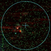 |
Fig. 1. WISE colour image centred on Upper Scorpius with TGAS objects overlaid, as seen in ESASky (Baines et al. 2017). The circle denotes the 10° surrounding the centre of Upper Scorpius. North is up, and east is left. |
The clustering analysis was performed using the DBSCAN algorithm as implemented in scikit-learn (Pedregosa et al. 2011). The source code used in our analysis can be found in Wilkinson (2017). At a high level, DBSCAN first identifies so-called core points at the centre of probable clusters, then expands outwards from these points until it reaches low-density noise. The algorithm uses two main parameters ε (eps) and minPts. Core points are defined as those with at least minPts neighbours within a radius of ε. Additional density-reachable points are added to a cluster if they are within a radius of ε (eps) from a core point of that cluster.
The dimensions used in DBSCAN were proper motion in right ascension and declination, and distance, since we are looking for clusters of co-moving stars at similar distances. The data in each dimension of the data set was standardised such that it had a mean of 0 and a variance of 1 for the clustering analysis. This allows the data in different dimensions to be compared. The DBSCAN algorithm requires a distance metric be set, in addition to ε (eps) and minPts. A Euclidian metric was used, which is the scikit-learn default.
Ester et al. (1996) describe a simple method to determine suitable values of minPts and eps, using a sorted k-distance graph. A sorted k-distance graph shows the distance to the kth nearest neighbour for each point in descending order. In this method, minPts is decided (from understanding of the data or otherwise), and the k-distance graph is generated with k set as minPts. This graph should have a valley at the threshold point between noise and clusters. The value of the sorted k-distance graph at the first point at the bottom of this valley is then taken as the eps.
We set minPts to 15 to minimise false positive clusters. In Appendix B we explore the behaviour of DBSCAN for other values of minPts. A suitable value of the eps for this value of minPts was then determined using the method described above. Figure 2 shows the sorted 15-distance graph obtained for the 2839 objects in the filtered data set and has a zoomed-in view of the valley inset. We compute the 15-distance in the dimensions we are clustering over: proper motion in right ascension and declination, and distance. A valley is clearly visible at around the 2700th point. We took the threshold point to be at the bottom of this valley. This gave us an eps of 1.103. We note that this threshold point is very far to the right of this graph since there is a large quantity of noise (i.e. objects not in the Upper Scorpius cluster) present.
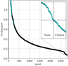 |
Fig. 2. Sorted 15-distance graph with a zoomed-in view of the threshold point between noise (left) and the cluster (right) inset. |
We validated this observed threshold point using a similar method to Gaia Collaboration (2016) to select a cluster in proper motion space manually, thereby estimating the size of the cluster associated with Upper Scorpius. This allowed us to estimate what percentage of the data is noise, and therefore where the valley in the 15-distance graph associated with the threshold point should be observed.
We plotted the data in proper motion space using the Tool for OPerations on Catalogues And Tables (TOPCAT) software package (Taylor 2005), and observed a rough cluster at a proper motion of around −10 mas yr−1 in right ascension and a −24 mas yr−1 in declination. The cluster was selected by manually drawing a boundary in TOPCAT. The selected cluster was observed to have 270 members, which gives us an estimate for the percentage of noise (i.e. objects not in Upper Scorpius) of 90%. We therefore expect to see the threshold point at around the 2600th point, which is as observed. We note that the observed threshold point is further to the right, since we expect to select fewer points when clustering with distance in addition to proper motion. Given that clustering is being performed over distance and proper motion, we are likely to be removing false positives compared to proper motion analysis alone.
Using an eps of 0.103 and a minPts of 15, we ran DBSCAN over the 2827 objects in the filtered data set. From this data set, DBSCAN selected one cluster with 167 members. These 167 member candidates are given in Table 1. Figures 3 and 4 show this cluster in proper motion space and in the sky plane. Figure 5 shows the distribution of the parallaxes for the filtered sample of 2827 objects, and for the cluster. We used Scott’s rule (Robitaille et al. 2013) to calculate suitable bin widths for the histogram. The cluster is very well defined in proper motion space and in terms of parallax. The median parallax of the cluster is 6.84 mas and has a mean relative parallax error (σπ/π) of 0.0947.
Member candidates of Upper Scorpius, including their SIMBAD ID.
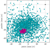 |
Fig. 3. Proper motion plot with members of the cluster selected by DBSCAN shown as pink squares. |
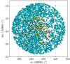 |
Fig. 4. Plot of the sky plane, with newly identified member candidates shown as pink triangles, and previously identified members of Scorpius-Centaurus shown as yellow squares. The boxes in the centre of the plot show the extent of several previous membership studies of ρ-Ophiuchi. Orange: Natta et al. (2002), green: Wilking et al. (2005), red: de Oliveira et al. (2010), blue: Erickson et al. (2011), black: Ducourant et al. (2017). North is up, and east is left. |
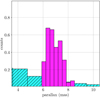 |
Fig. 5. Parallax histogram for all objects (blue, hatched), and the members of the cluster selected by DBSCAN (pink) |
The mean distance of the member candidates 145.9 ± 7.5 pc. We note that 7.5 pc is the standard error of the mean. The distance distribution of the member candidates extends from ∼120– 165 pc, suggesting a spread of ∼45 pc in distance. We also obtain a mean proper motion of (−11.4, −23.5) ± (0.7, 0.4) mas yr−1. de Zeeuw et al. (1999) estimates the distance to Upper Scorpius at 145 ± 2.5 pc and the mean proper motion to be (−8.1, −24.5) ± (0.1, 0.1) mas yr−1. Preibisch & Mamajek (2008) suggested a maximum spread in distance of ∼50 pc. Galli et al. (2018), using data from Gaia DR1, obtained a mean distance of 146 ± 3 ± 6 pc. The consistency of the member candidates with these estimates suggests a high probability of membership in Upper Scorpius.
In order to identify the effect of brightness binning on the mean distance of the cluster, the clustering was re-run on subsamples of the data with G-band mean magnitude above and below 10 mag. Since the vast majority of the candidate members had a magnitude greater than 10 mag (128 out of 167), no cluster was selected for the subsample with a magnitude less than 10 mag. For the subsample with magnitude greater than 10 mag, a cluster of 127 objects was selected with a mean distance of 146.1 pc. This is nearly identical to the mean distance for candidate members. This shows that any potential bias in the mean distance of the member candidates, and therefore in member selection, is not severe.
3. Discussion
We first cross-matched the member candidates with the Set of Identifications, Measurements, and Bibliography for Astronomical Data (SIMBAD) catalogue, using a radius of 2 arcsec. This found corresponding SIMBAD objects for each member candidate, and accordingly the object name is included as a field in Table 1. We then cross-matched the member candidates with members of Scorpius-Centaurus from Chen et al. (2012), Pecaut et al. (2012), Luhman & Mamajek (2012), Rizzuto (2015), and Pecaut & Mamajek (2016). Of the 167 member candidates, 89 are previously identified members of Upper Scorpius. Additionally, 2 are previously identified members of Upper Centaurus-Lupus. This gives us 78 newly identified member candidates of Upper Scorpius. Given that the mean distance and mean proper motion of the candidate members are consistent with existing estimates, we are confident that we have selected strong member candidates of Upper Scorpius.
We then compared the member candidates with previous stellar kinematics-based member selection methods applied to Upper Scorpius. Cross-matching the 167 member candidates with those from de Zeeuw et al. (1999) found 55 members in common. Of the members identified by de Zeeuw et al. (1999), 80 are present in TGAS. Similarly, cross-matching with Hoogerwerf & Aguilar (1999) found 107 members in common. Of the members identified by Hoogerwerf & Aguilar (1999), 244 are present in TGAS. Cross-matching with Rizzuto et al. (2011) found 49 members in common. Of the members identified by Rizzuto et al. (2011), 74 are present in TGAS. Figure 6 compares the proper motion distribution of the member candidates with members previously identified by de Zeeuw et al. (1999), Hoogerwerf & Aguilar (1999), and Rizzuto et al. (2011) that are present within TGAS and in the target region. This shows that DBSCAN can successfully recover the core of the proper motion distribution of a cluster, but struggles at the low-density extremes. This is understandable, since outside the core of the distribution the background stars provide a substantial amount of noise. Figure 6 suggests that those objects not re-selected by DBSCAN are outside this core, which explains the discrepancy in re-selection of previous kinematically selected members. As a result, detailed analysis of the kinematic structure of the selected member candidates is not appropriate since we are selecting members from the core of the velocity distribution. The newly selected member candidates were possibly missed by previous kinematic analyses because of the systematically worse parallax uncertainties of HIPPARCOS (median of 0.97 mas) compared to TGAS (median of 0.32 mas). The unique nature of the DBSCAN algorithm as compared with previous methods, as described in Sect. 1, may have also played a role. It is worth noting that while the proper motion uncertainties of HIPPARCOS (median of (0.88, 0.74) mas yr−1) are better than TGAS (median of (1.32, 1.32) mas yr−1), the uncertainties of the HIPPARCOS subset of TGAS (median of (0.07, 0.07) mas yr−1) and the member candidates (median of (0.51, 0.39) mas yr−1) are systematically better than both.
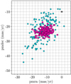 |
Fig. 6. Proper motion plot, with members of the cluster selected by DBSCAN shown as pink squares. Previously identified members of Upper Scorpius from de Zeeuw et al. (1999), Hoogerwerf & Aguilar (1999), and Rizzuto et al. (2011) that are also present in the TGAS catalogue, are show as blue circles. |
From Fig. 3, we can see that the cluster of candidate members has a width of approximately 5 mas yr−1 in proper motion space. Two objects with a relative proper motion of 5 mas yr−1 would end up 10° apart after 7.2 Myr. Therefore the radius of the cone used for the selection of data from the TGAS catalogue likely includes the entirety of Upper Scorpius, given the probable young age of the region (∼10 Myr, Pecaut et al. 2012; Feiden 2016).
Upper Scorpius is in very close proximity to the ρ-Ophiuchus molecular cloud (Preibisch & Mamajek 2008), so there is the potential for ρ-Ophiuchus members to contaminate the sample. However, Fig. 4 shows that none of the member candidates of Upper Scorpius selected by DBSCAN are present in the areas of ρ-Ophiuchi observed by Natta et al. (2002), Wilking et al. (2005), de Oliveira et al. (2010), or Erickson et al. (2011), so there are no common objects.
The distribution of the distances within the member candidates is possibly bimodal with apparent peaks at approximately 154 pc (6.5 mas) and 133 pc (7.5 mas). While we could not establish the significance of this, a more complete sample of members may show significant bimodality. It should also be noted that there are very few member candidates that lie in the upper-right (north–west) of the sky plane of the region studied. Previous work has suggested possible substructure within the subgroups of Scorpius-Centaurus. Rizzuto et al. (2011) could not determine non-arbitrary boundaries between the subgroups of Scorpius-Centaurus owing to blurring from velocity dispersion. Through producing an age map of Scorpius-Centaurus, Pecaut & Mamajek (2016) found potential evidence of substructure within the older subgroups of the complex (Upper Centaurus-Lupus and Lower Centaurus-Crux). Using kinematic data from Gaia DR1 and HIPPARCOS, Wright & Mamajek (2018) found evidence of kinematic substructure within the subgroups of Scorpius-Centaurus. Additionally, the 3D structure of Upper Scorpius obtained by Galli et al. (2018) from Gaia DR1 supports bimodality. Further investigation of this substructure could prove fruitful, especially with data from Gaia DR2.
In Appendix A, we discuss the performance of DBSCAN applied to two sets of 20 simulations: one set produced by binning the data and uniformly generating data within those bins, and the other produced by modelling the cluster and the background as Gaussian. We estimated the number of likely contaminants to be ∼6–17 (∼3.8–10.2%).
4. Conclusions
We applied DBSCAN to the set of TGAS objects within a 10° radius surrounding Upper Scorpius, selecting 167 candidate members. Of these member candidates, 89 are previously identified members of Upper Scorpius and 2 are previously identified members of Upper Centaurus-Lupus. The member candidates have a mean distance of 145.6 ± 7.5 pc, a spread of ∼45 pc in distance, and a proper motion of (−11.4, −23.5) ± (0.7, 0.4) mas yr−1 that is consistent with previous estimates for Upper-Scorpius. This suggests a strong likelihood of true membership of Upper Scorpius. In Appendix A we estimated the number of likely contaminants to be ∼6–17 (∼3.8–10.2%).
While the distance distribution of member candidates suggests possible kinematic substructure in Upper Scorpius, the significance of this finding has not yet been established. Unlike many established stellar kinematics-based member selection methods, DBSCAN does not attempt to model the internal motion of associations and relies on density alone. With the increase in precision of parallaxes and proper motions from Gaia, non-trivial substructure within associations can be investigated effectively. As a density-based clustering algorithm, DBSCAN is resilient to these substructures, so is well suited to identify them. However, while it can effectively recover the core of the proper motion distribution of an association, it struggles at the low-density fringes compared to established methods.
Analysing the colour, geometric, and spectral energy distributions of the new candidate members could prove to be fruitful, but these paths are beyond the scope of this work. The 78 new candidate members should be followed up spectroscopically for their true membership to be confirmed. Were some of the new candidate members to be confirmed as true members, they would be prime candidates for ALMA imaging searches for protoexoplanets embedded in their potential protoplanetary discs.
Acknowledgments
This work has made use of data from the European Space Agency (ESA) mission Gaia (http://www.cosmos.esa.int/gaia), processed by the Gaia Data Processing and Analysis Consortium (DPAC, http://www.cosmos.esa.int/web/gaia/dpac/consortium). Funding for the DPAC has been provided by national institutions, in particular the institutions participating in the Gaia Multilateral Agreement. This work has made use of ESASky, developed by the ESAC Science Data Centre (ESDC) team and maintained alongside other ESA science mission’s archives at ESA’s European Space Astronomy Centre (ESAC, Madrid, Spain). This research made use of matplotlib, a Python library for publication quality graphics (Hunter 2007). This research made use of NumPy (van der Walt et al. 2011). This research made use of SciPy (Jones et al. 2001). This research made use of Scikit-learn (Pedregosa et al. 2011). This research made use of Astropy, a communitydeveloped core Python package for Astronomy (Astropy Collaboration 2013). This research made use of TOPCAT, an interactive graphical viewer and editor for tabular data (Taylor 2005). This work has made use of the SIMBAD database, operated at CDS, Strasbourg, France. This research has made use of the VizieR catalogue access tool, CDS, Strasbourg, France (Ochsenbein et al. 2000).
Appendix A: Cluster simulation and recovery
In order to verify the suitability of the DBSCAN for the purpose of this analysis, we applied our method to two sets of simulations. One set was produced by binning the data and the other by modelling the cluster and background as Gaussian. We simulated the cluster selected by DBSCAN and the remaining background stars independently. In the binning method, for each group, the data was binned over distance and proper motion in right ascension and declination using the bin width obtained by the Rice rule (Jones et al. 2001) applied to the cluster. Simulated data for each bin was then generated using a random uniform distribution in each dimension.
For each sample, a sorted k-distance graph was created, and the eps was identified. We then applied the DBSCAN algorithm to the simulated data using the identified eps and a minPts of 15. The cluster selected by DBSCAN from the simulated data was then analysed to determine the number of false positives (objects not in the simulated cluster, selected by DBSCAN) and false negatives (objects in the simulated cluster, not selected by DBSCAN). The percentage of false positives was calculated from the number of false positives over the size of the cluster selected by DBSCAN, and the percentage of false negatives was calculated from the number of false negatives over the size of the simulated cluster. This process was repeated 20 times for each simulation method. For the binning method, we obtained a mean false positive percentage of 10.2% and false negative percentage of 5.1%. For the Gaussian method, we obtained a mean false positive percentage of 3.8% and false negative percentage of 6.0%. Figures A.1 and A.2 illustrate a sample of the results of DBSCAN performed on the data simulated using the binning method and Gaussian method, respectively.
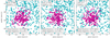 |
Fig. A.1. Proper motion plots showing the results of DBSCAN performed on three samples of data simulated with the binning method. True cluster members are represented by squares, and true background objects by circles. Objects selected by DBSCAN are shown in pink. |
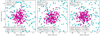 |
Fig. A.2. Proper motion plots showing the results of DBSCAN performed on three samples of data simulated with the Gaussian method. True cluster members are represented by squares, and true background objects by circles. Objects selected by DBSCAN are shown in pink. |
As discussed in Sect. 3 and illustrated by Fig. 6, DBSCAN can successfully recover the core of the proper motion distribution of a cluster, but struggles at the low-density extremes. Therefore for the Gaussian simulation, DBSCAN likely recovers the core of the simulated Gaussian distribution effectively, resulting in a lower false positive rate. With the binning method, since we simulate the distribution of the original member candidates, we are attempting re-select the core of the distribution directly without a surrounding distribution. Compared to the Gaussian method, the binning method likely has a higher false positive rate. These two methods provide a possible range for the number of likely contaminants in the member candidates, with the Gaussian simulation as a lower bound and the binning simulation as an upper bound. This gives a range of likely contaminants of ∼6–17 (∼3.8–10.2%).
Appendix B: DBSCAN parameter sensitivity
In order to demonstrate the behaviour of DBSCAN under the variation of the parameters, we reran DBSCAN on the data for different combinations of eps and minPts. Figure B.1 shows the results, in proper motion space, of 12 different parameter combinations. The top six plots vary the eps between 0.5 and 0.05 for a minPts of 15, which is the value of minPts used in our main analysis. We see that for an eps significantly larger than 0.103, the value determined from the k-distance graph, DBSCAN selects almost the entirety of the data as a single cluster. The cluster selected collapses inwards as the eps is lowered towards 0.103. For an eps of 0.05, DBSCAN selects a small portion of the core of the cluster associated with Upper Scorpius.
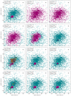 |
Fig. B.1. Proper motion plots showing the results of DBSCAN performed, with various combinations of parameters, on the TGAS sample. Background objects are shown in blue; each cluster is shown in a different colour. If more than 7 clusters are selected, the excess clusters are all shown in grey. |
The bottom six plots vary minPts to 5, 30, and 50, showing the results of DBSCAN for an eps of 0.103, as used for a minPts of 15, and for the value determined for each minPts from their respective k-distance graph. We see that for a minPts of 5, an extremely large number of clusters are selected, 33 for an eps of 0.103 and 12 for an eps of 0.064. This is because minPts is too small, so DBSCAN selects small-scale over-densities in the data that most likely do not correspond to any meaningful structure. For a minPts of 30 and 50, with an eps of 0.103, which in this case is too small a value, DBSCAN will select a subset of the cluster associated with Upper Scorpius. With the eps selected by the k-distance graph for each case, the clusters are much closer to that obtained in our main analysis.
References
- Astropy Collaboration (Robitaille, T. P., et al.) 2013, A&A, 558, A33 [NASA ADS] [CrossRef] [EDP Sciences] [Google Scholar]
- Baines, D., Giordano, F., Racero, E., et al. 2017, PASP, 129, 028001 [NASA ADS] [CrossRef] [Google Scholar]
- Chen, C. H., Pecaut, M., Mamajek, E. E., Su, K. Y. L., & Bitner, M. 2012, ApJ, 756, 133 [NASA ADS] [CrossRef] [Google Scholar]
- de Bruijne, J. H. J. 1999, MNRAS, 306, 381 [NASA ADS] [CrossRef] [Google Scholar]
- de Oliveira, C. A., Moraux, E., Bouvier, J., et al. 2010, A&A, 515, A75 [NASA ADS] [CrossRef] [EDP Sciences] [Google Scholar]
- de Zeeuw, P. T., Hoogerwerf, R., de Bruijne, J. H. J., Brown, A. G. A., & Blaauw, A. 1999, AJ, 117, 354 [NASA ADS] [CrossRef] [Google Scholar]
- Dehnen, W., & Binney, J. J. 1998, MNRAS, 298, 387 [NASA ADS] [CrossRef] [Google Scholar]
- Ducourant, C., Teixeira, R., Krone-Martins, A., et al. 2017, A&A, 597, A90 [NASA ADS] [CrossRef] [EDP Sciences] [Google Scholar]
- Erickson, K. L., Wilking, B. A., Meyer, M. R., Robinson, J. G., & Stephenson, L. N., 2011, AJ, 142, 140 [NASA ADS] [CrossRef] [Google Scholar]
- Ester, M., Kriegel, H. P., Sander, J., & Xu, X. 1996, in Proceedings of the Second International Conference on Knowledge Discovery and Data Mining (AAAI Press), 226 [Google Scholar]
- Feiden, G. A. 2016, A&A, 593, A99 [NASA ADS] [CrossRef] [EDP Sciences] [Google Scholar]
- Gagné, J., Lafreniére, D., Doyon, R., Malo, L., & Artigau, E. 2013, AJ, 783, 121 [Google Scholar]
- Gaia Collaboration (Prusti, T., et al.) 2016, A&A, 595, A1 [NASA ADS] [CrossRef] [EDP Sciences] [Google Scholar]
- Galli, P. A. B., Joncour, I., & Moraux, E. 2018, MNRAS, 477, L50 [NASA ADS] [CrossRef] [Google Scholar]
- Hoogerwerf, R., & Aguilar, L. A. 1999, MNRAS, 306, 394 [NASA ADS] [CrossRef] [Google Scholar]
- Hunter, J. D. 2007, Comput. Sci. Eng., 9, 90 [Google Scholar]
- Jones, E., Oliphant, T., & Peterson, P. 2001, SciPy: Open Source Scientific Tools for Python, http://www.scipy.org/ [Google Scholar]
- Lépine, S., & Simon, M. 2009, AJ, 137, 3632 [NASA ADS] [CrossRef] [Google Scholar]
- Luhman, K. L., & Mamajek, E. E. 2012, ApJ, 758, 31 [NASA ADS] [CrossRef] [Google Scholar]
- Malo, L., Doyon, R., Lafrenière, D., et al. 2013, ApJ, 762, 88 [NASA ADS] [CrossRef] [Google Scholar]
- Michalik, D., Lindegren, L., & Hobbs, D. 2015, A&A, 574, A115 [NASA ADS] [CrossRef] [EDP Sciences] [Google Scholar]
- Natta, A., Testi, L., Comerón, F., et al. 2002, A&A, 393, 597 [NASA ADS] [CrossRef] [EDP Sciences] [Google Scholar]
- Ochsenbein, F., Bauer, P., & Marcout, J. 2000, A&AS, 143, 23 [NASA ADS] [CrossRef] [EDP Sciences] [Google Scholar]
- Pecaut, M. J., & Mamajek, E. E. 2016, MNRAS, 461, 794 [NASA ADS] [CrossRef] [Google Scholar]
- Pecaut, M. J., Mamajek, E. E., & Bubar, E. J. 2012, ApJ, 746, 154 [NASA ADS] [CrossRef] [Google Scholar]
- Pedregosa, F., Varoquaux, G., Gramfort, A., et al. 2011, J. Mach. Learn. Res., 12, 2825 [Google Scholar]
- Platais, I., Kozhurina-Platais, V., & van Leeuwen, F. 1998, AJ, 116, 2423 [NASA ADS] [CrossRef] [Google Scholar]
- Preibisch, T., & Mamajek, E., 2008, The Nearest OB Association: Scorpius-Centaurus, ed. B. Reipurth (San Francisco, CA: ASP Mono. Pub.), 235 [Google Scholar]
- Rizzuto, A. 2015, AAS/Division for Extreme Solar Systems Abstracts, 3, 120.03 [Google Scholar]
- Rizzuto, A. C., Ireland, M. J., & Robertson, J. G. 2011, MNRAS, 416, 3108 [NASA ADS] [CrossRef] [Google Scholar]
- Robitaille, T. P., Tollerud, E. J., Greenfield, P., et al. 2013, A&A, 558, A33 [NASA ADS] [CrossRef] [EDP Sciences] [Google Scholar]
- Taylor, M. B. 2005, in ASP Conf. Ser., 347, 29 [Google Scholar]
- van der Walt, S., Colbert, S. C., & Varoquaux, G. 2011, Comp. Sci. - Math. Soft., DOI: 10.1109/MCSE.2011.37 [Google Scholar]
- Wilking, B. A., Meyer, M. R., Robinson, J. G., & Greene, T. P. 2005, AJ, 130, 1733 [NASA ADS] [CrossRef] [Google Scholar]
- Wilkinson, S. 2017, Clustering Analysis of Ophiuchus-Scorpius using DBSCAN, https://github.com/scwilkinson/DBSCAN-Upper-Scorpius [Google Scholar]
- Wright, N. J., & Mamajek, E. E. 2018, MNRAS, 476, 381 [NASA ADS] [CrossRef] [Google Scholar]
All Tables
All Figures
|
Fig. 1. WISE colour image centred on Upper Scorpius with TGAS objects overlaid, as seen in ESASky (Baines et al. 2017). The circle denotes the 10° surrounding the centre of Upper Scorpius. North is up, and east is left. |
| In the text | |
|
Fig. 2. Sorted 15-distance graph with a zoomed-in view of the threshold point between noise (left) and the cluster (right) inset. |
| In the text | |
|
Fig. 3. Proper motion plot with members of the cluster selected by DBSCAN shown as pink squares. |
| In the text | |
|
Fig. 4. Plot of the sky plane, with newly identified member candidates shown as pink triangles, and previously identified members of Scorpius-Centaurus shown as yellow squares. The boxes in the centre of the plot show the extent of several previous membership studies of ρ-Ophiuchi. Orange: Natta et al. (2002), green: Wilking et al. (2005), red: de Oliveira et al. (2010), blue: Erickson et al. (2011), black: Ducourant et al. (2017). North is up, and east is left. |
| In the text | |
|
Fig. 5. Parallax histogram for all objects (blue, hatched), and the members of the cluster selected by DBSCAN (pink) |
| In the text | |
|
Fig. 6. Proper motion plot, with members of the cluster selected by DBSCAN shown as pink squares. Previously identified members of Upper Scorpius from de Zeeuw et al. (1999), Hoogerwerf & Aguilar (1999), and Rizzuto et al. (2011) that are also present in the TGAS catalogue, are show as blue circles. |
| In the text | |
|
Fig. A.1. Proper motion plots showing the results of DBSCAN performed on three samples of data simulated with the binning method. True cluster members are represented by squares, and true background objects by circles. Objects selected by DBSCAN are shown in pink. |
| In the text | |
|
Fig. A.2. Proper motion plots showing the results of DBSCAN performed on three samples of data simulated with the Gaussian method. True cluster members are represented by squares, and true background objects by circles. Objects selected by DBSCAN are shown in pink. |
| In the text | |
|
Fig. B.1. Proper motion plots showing the results of DBSCAN performed, with various combinations of parameters, on the TGAS sample. Background objects are shown in blue; each cluster is shown in a different colour. If more than 7 clusters are selected, the excess clusters are all shown in grey. |
| In the text | |
Current usage metrics show cumulative count of Article Views (full-text article views including HTML views, PDF and ePub downloads, according to the available data) and Abstracts Views on Vision4Press platform.
Data correspond to usage on the plateform after 2015. The current usage metrics is available 48-96 hours after online publication and is updated daily on week days.
Initial download of the metrics may take a while.