| Issue |
A&A
Volume 616, August 2018
|
|
|---|---|---|
| Article Number | A174 | |
| Number of page(s) | 15 | |
| Section | Extragalactic astronomy | |
| DOI | https://doi.org/10.1051/0004-6361/201833047 | |
| Published online | 03 September 2018 | |
The VANDELS ESO public spectroscopic survey: Observations and first data release
1
INAF-Osservatorio Astronomico di Roma,
via Frascati 33,
00078
Monteporzio Catone,
Italy
e-mail: laura.pentericci@oa-roma.inaf.it
2
Institute for Astronomy, University of Edinburgh, Royal Observatory,
Edinburgh
EH9 3HJ,
UK
3
INAF-Istituto di Astrofisica Spaziale e Fisica Cosmica Milano,
via Bassini 15,
20133
Milano,
Italy
4
INAF-Osservatorio di Astrofisica e Scienza dello Spazio di Bologna,
via Gobetti 93/3,
40129
Bologna,
Italy
5
INAF-Osservatorio Astronomico di Brera,
via Brera 28,
20122
Milano,
Italy
6
Kavli Institute for Cosmology, University of Cambridge,
Madingley Road,
Cambridge
CB3 0HA,
UK
7
Cavendish Laboratory, University of Cambridge,
19 J. J. Thomson Avenue,
Cambridge
CB3 0HE,
UK
8
Dipartimento di Fisica e Astronomia, Università degli Studi di Bologna,
Via Piero Gobetti 93/2,
40129
Bologna,
Italy
9
INAF-Osservatorio Astrofisico di Arcetri,
Largo E. Fermi 5,
50157
Firenze,
Italy
10
European Southern Observatory,
Karl-Schwarzschild-Str. 2,
85748
Garching b. München,
Germany
11
Observatoire de Genève, Université de Genève,
51 Ch. des Maillettes,
1290
Versoix,
Switzerland
12
Laboratoire AIM Paris-Saclay, CEA/DSM/Irfu, CNRS,
91191
Gifsur-Yvette,
France
13
Department of Astronomy, The University of Texas at Austin,
Austin,
TX 78712,
USA
14
INAF-Astronomical Observatory of Trieste,
via G.B. Tiepolo 11,
34143
Trieste,
Italy
15
Núcleo de Astronomía, Facultad de Ingeniería, Universidad Diego Portales,
Av. Ej’ercito 441,
Santiago,
Chile
16
Department of Physics and Astronomy, University College London,
Gower Street,
London
WC1E 6BT,
UK
17
Astrophysics, The Denys Wilkinson Building, University of Oxford,
Keble Road,
Oxford
OX1 3RH,
England
18
Kapteyn Astronomical Institute, University of Groningen,
Postbus 800,
9700 AV
Groningen,
The Netherlands
19
Max Planck Institut für Extraterrestrische Physik,
Giessenbachstrasse 1,
Garching
85748,
Germany
20
European Southern Observatory, Avenida Alonso de Córdova 3107,
Vitacura,
19001
Casilla,
Santiago de Chile,
Chile
21
School of Physics and Astronomy, University of Nottingham, University Park,
Nottingham
NG7 2RD,
UK
22
University Observatory Munich,
Scheinerstrasse 1,
81679
Munich,
Germany
23
Department of Astronomy, University of Michigan,
311 West Hall, 1085 South University Ave.,
Ann Arbor,
MI 48109-1107,
USA
24
Instituto de Astrofísica e Ciências do Espaço, Universidade de Lisboa, OAL, Tapada da Ajuda,
1349-018
Lisbon,
Portugal
25
Departamento de Física, Faculdade de Ciências, Universidade de Lisboa, Edifício C8, Campo Grande,
1749-016
Lisbon,
Portugal
26
Instituto de Fisica y Astronomia, Facultad de Ciencias, Universidad de Valparaiso,
1111
Gran Bretana,
Valparaiso,
Chile
27
Institute d’Astrophysique de Paris, CNRS, Université Pierre et Marie Curie,
98 bis Boulevard Arago,
75014
Paris,
France
28
National Optical Astronomy Observatory,
950 North Cherry Ave,
Tucson,
AZ
85719,
USA
29
Harvard-Smithsonian Center for Astrophysics,
60 Garden St,
Cambridge
MA 20138,
England
30
Space Telescope Science Institute,
3700 San Martin Drive,
Baltimore,
MD
21218,
USA
31
The Cosmic Dawn Center, Niels Bohr Institute, University of Copenhagen,
Juliane Maries Vej 30,
2100
Copenhagen,
Denmark
32
Astronomy Department, University of Massachusetts,
Amherst,
MA 01003,
USA
33
Instituto de Astrofísica Avda. Pontificia Universidad Católica de Chile, Vicuña Mackenna,
4860
Santiago,
Chile
34
Aix-Marseille Université, CNRS, LAM (Laboratoire d’Astrophysique de Marseille) UMR 7326,
13388
Marseille,
France
35
Instituto de Astrofísica de Canarias,
Calle Vía Láctea s/n,
38205
La Laguna,
Tenerife,
Spain
36
Departamento de Astrofísica, Universidad de La Laguna,
38200
La Laguna,
Tenerife,
Spain
37
Faculty of Physics, Ludwig-Maximilians Universität,
Scheinerstr. 1,
81679
Munich,
Germany
38
Department of Physics and Astronomy, Texas A&M University,
College Station,
TX 77843-4242,
USA
39
Excellence Cluster,
Boltzmannstr. 2,
85748
Garching,
Germany
40
Department of Physics, Durham University,
South Road,
DH1 3LE
Durham,
UK
41
Leiden Observatory, Leiden University,
2300 RA
Leiden,
The Netherlands
42
Steward Observatory, The University of Arizona,
933 N Cherry Ave,
Tucson,
AZ
85721,
USA
43
Department of Physics and Astronomy,
PAB,
430 Portola Plaza, Box 951547,
Los Angeles,
CA 90095-1547,
USA
44
School of Physics and Astronomy, University of St. Andrews, SUPA,
North Haugh,
KY16 9SS
St. Andrews,
UK
Received:
19
March
2018
Accepted:
2
May
2018
This paper describes the observations and the first data release (DR1) of the ESO public spectroscopic survey “VANDELS, a deep VIMOS survey of the CANDELS CDFS and UDS fields”. The main targets of VANDELS are star-forming galaxies at redshift 2.4 < z < 5.5, an epoch when the Universe had not yet reached 20% of its current age, and massive passive galaxies in the range 1 < z < 2.5. By adopting a strategy of ultra-long exposure times, ranging from a minimum of 20 h to a maximum of 80 h per source, VANDELS is specifically designed to be the deepest-ever spectroscopic survey of the high-redshift Universe. Exploiting the red sensitivity of the refurbished VIMOS spectrograph, the survey is obtaining ultra-deep optical spectroscopy covering the wavelength range 4800–10 000 Å with a sufficiently high signal-to-noise ratio to investigate the astrophysics of high-redshift galaxy evolution via detailed absorption line studies of well-defined samples of high-redshift galaxies. VANDELS-DR1 is the release of all medium-resolution spectroscopic data obtained during the first season of observations, on a 0.2 square degree area centered around the CANDELS-CDFS (Chandra deep-field south) and CANDELS-UDS (ultra-deep survey) areas. It includes data for all galaxies for which the total (or half of the total) scheduled integration time was completed. The DR1 contains 879 individual objects, approximately half in each of the two fields, that have a measured redshift, with the highest reliable redshifts reaching zspec ~ 6. In DR1 we include fully wavelength-calibrated and flux-calibrated 1D spectra, the associated error spectrum and sky spectrum, and the associated wavelength-calibrated 2D spectra. We also provide a catalog with the essential galaxy parameters, including spectroscopic redshifts and redshift quality flags measured by the collaboration. We present the survey layout and observations, the data reduction and redshift measurement procedure, and the general properties of the VANDELS-DR1 sample. In particular, we discuss the spectroscopic redshift distribution and the accuracy of the photometricredshifts for each individual target category, and we provide some examples of data products for the various target typesand the different quality flags. All VANDELS-DR1 data are publicly available and can be retrieved from the ESO archive. Two further data releases are foreseen in the next two years, and a final data release is currently scheduled for June 2020, which will include an improved rereduction of the entire spectroscopic data set.
Key words: surveys / galaxies: general / galaxies: evolution / galaxies: high-redshift / galaxies: fundamental parameters
© ESO 2018
1 Introduction
Significant progress in our understanding of galaxy formation and evolution requires observations of substantial samples of galaxies over a large enough volume and a wide range of masses and redshifts. Only with representative samples and reliable observations are we able to test models of galaxy formation in a rigorous way. In particular, spectroscopic surveys can play a key role because in addition to accurate information on the galaxy redshifts, they provide a wealth of other important observable properties, such as emission and absorption line features, measures of internal motions, spectral indices, and spectral breaks. These in turn allow us to characterize the intrinsic physical properties of galaxies and the nature of their stellar populations, including the chemical composition, non-thermal sources, the ionizing radiation field, and the evolution of all these properties with cosmic time (Ellis et al. 2017).
In recent years, a series of spectroscopic campaigns has been carried out, starting from the low-redshift Universe, where the Sloan Digital Sky Survey (SDSS) observed more than a million galaxies at redshifts z ~ 0.1−0.7 (Alam et al. 2015; Reid et al. 2016). At redshifts z ~ 1, a series of spectroscopic surveys has sampled large volumes of the Universe by observing many tens of thousands of galaxies: in this redshift range, the Very Large Telescope (VLT) and the VIsible MultiObject Spectrograph (VIMOS) have played a major role, with the VIMOS Very Deep Survey (VVDS; Le Fèvre et al. 2005), the COSMOS spectroscopic survey (zCOSMOS; Lilly et al. 2007), and the VIMOS Public Extragalactic Redshift Survey (VIPERS; Guzzo et al. 2014). These surveys contributed substantially to improving our understanding of galaxy evolution also in relation to the environment. At even higher redshift (z > 2), spectroscopic surveys have been necessarily more limited, and at most several thousand galaxies have been identified at z ~ 2−4 (e.g., KBSS-MOSFIRE; Steidel et al. 2014, and VUDS; Le Fèvre et al. 2015), which become fewer than a few hundred galaxies toward the reionization epoch at z ≥ 5 (De Barros et al. 2017; Shibuya et al. 2018; Pentericci et al. 2018). The main aim of these surveys has been the redshift identification of increasingly distant (and faint) galaxies, particularly star-forming objects. A somewhat complementary approach was employed by the Galaxy Mass Assembly ultra-deep Spectroscopic Survey (GMASS; Cimatti et al. 2008; Kurk et al. 2013), which investigated the physical and evolutionary processes of galaxy mass assembly in the redshift range of 1.5 < z < 3 by obtaining ultra-deep optical spectra (up to 32 h). This allowed a detailed spectral study of a small sample of passive galaxies at z ~ 1.5 and several tens of star-forming galaxies up to z ~ 3.
VANDELS, a VIMOS survey of the CANDELS CDFS (Chandra deep-field south) and UDS (ultra-deep survey) fields, is an ESO public spectroscopic survey designed to complement and extend the work of these previous campaigns by focusing on ultra-long exposures of a relatively small number of galaxies that were preselected to lie at high redshift. VANDELS started observations in August 2015 and was completed in February 2018. Exploiting the red sensitivity of the refurbished VIMOS spectrograph and ultra-long integration times of up to 80 h on source, the survey is obtaining ultra-deep optical spectroscopy of around 2100 galaxies in the redshift interval 1.0 < z < 7.0, including star-forming galaxies at redshift z > 2.4, an epoch when the Universe had not yet reached 20% of its current age and massive passive galaxies in the range 1 < z < 2.5. VANDELS has observed in the wavelength range 4800–10 000 Å with intermediate resolution. The prime motivation is to move beyond simple redshift acquisition by obtaining spectra with high enough signal-to-noise ratio (S/N) to allow detailed absorption and emission line studies in individual spectra, derive metallicities and velocity offsets, and finally derive improved constraints on physical parameters, such as stellar mass and star formation rates. This information will enable a detailed investigation of the physics of galaxies in the early Universe. By targeting two extragalactic survey fields with superb multiwavelength imaging data, including the best optical plus near-infrared (NIR) plus Spitzer imaging, VANDELS will produce a unique legacy data set for exploring the physics underpinning high-redshift galaxy evolution.
After a brief summary of the target selection (Sect. 2), we present the survey layout and observations (Sect. 3), the data reduction process (Sect. 4), the redshift measurement procedure (Sect. 5), and, finally, the content of DR1 (Sect. 6) with the general description of the data that are publicy available, the properties of the galaxies in the release, and some examples of data products fordifferent types of galaxies. In a companion paper (McLure et al. 2018), we present complementary information, including the main scientific motivations of the survey, the assembly of the photometric catalogs, the determination of the photometric redshifts, and the selection for the different target categories that were observed in the survey.
We refer to total magnitudes in the AB system (Oke & Gunn 1983). When quoting absolute quantities, we assume a cosmology with H0 = 70 km s−1 Mpc−1, ΩΛ = 0.7, and Ωm = 0.3.
2 The VANDELS public spectroscopic survey
We provide a brief summary of the survey below, but refer to McLure et al. (2018) for a detailed description of the target selection and survey definition. The VANDELS survey targets two fields, the UKIDSS Ultra Deep Survey (UDS: 02:17:38, –05:11:55) and the Chandra Deep Field South (CDFS: 03:32:30, –27:48:28). These fields were selected since their central areas have the best available Hubble Space Telescope (HST) multiwavelength data from the CANDELS treasury survey (Koekemoer et al. 2011; Grogin et al. 2011), as well as a wealth of ancillary data, including ultra-deep IRAC photometry.
For the CANDELS/HST areas (CDFS-HST and UDS-HST) we adopted the photometric catalogs that are based on H160 -band detections and are provided by the CANDELS team (Galametz et al. 2013; Guo et al. 2013) to select our targets. These catalogs provide point spread function (PSF) homogenized photometry for the available ACS and WFC3/IR (infrared) imaging, in addition to spatial-resolution matched photometry from Spitzer IRAC and key ground-based imaging data sets. Specifically, the CDFS-HST catalog includes photometry in 17 broadband filters (Guo et al. 2013), while the UDS-HST catalog includes photometry in 19 broadband filters (Galametz et al. 2013).
Because of the large field of view (FOV) of VIMOS, the spectroscopic observations also cover areas that are outside the original CANDELS footprints. For these wider-field areas (CDFS-GROUND and UDS-GROUND) no NIR-selected photometric catalogs are available, therefore, new multiwavelength photometric catalogs were assembled using the publicly available imaging. Briefly, these new multiwavelength photometric catalogs were generated using the publicly available imaging in 12 filters for UDS-GROUND and 17 filters for CDFS-GROUND, spanning the range from U to K band in both cases. The assembly of the new catalogs and the list of multiband data we employed are described together in detail in McLure et al. (2018).
For the two central regions that are covered by deep HST imaging, we adopted the photometric redshift solutions by the CANDELS survey team (Guo et al. 2013; Santini et al. 2015), which were derived by optimally combining several independent estimates produced by different photometric redshift codes by CANDELS team members, as described in detail in Dahlen et al. (2013). For the wider areas outside the CANDELS footprint, new photometric redshifts were generated by our team, based on the new photometric catalogs described above. Fourteen independent photometric redshift estimates were generated by 11 individual team members based on different codes and methods. They were then combined by taking the median value of zphot for each galaxy and producing an official VANDELS zphot.
The targets were then selected using the CANDELS and the new VANDELS photometric catalogs and photometric redshifts, respectively, for the areas with deep HST imaging and for the wider areas. Here, we briefly recall the main object categories that were selected.
- 1)
Bright star-forming galaxies (SFG): this sample consists of star-forming galaxies with i ≤ 25 with a best photometric redshift in the range 2.4 ≤ zphot ≤ 5.5 so that the main absorption features necessary to investigate the metallicity (e.g., as in Sommariva et al. 2012 and Rix et al. 2004) fall in the observed spectral range. In practice, the redshift range of the resulting sample is limited to zphot < 5. The galaxies were required to have sSFR > 0.1 Gyr−1, where sSFR is the specific star formation rate derived by the spectral energy distribution (SED) fitting described by McLure et al. (2018), assuming the best photometric redshift.
- 2)
Passive galaxies (PASS): this sample consists of UVJ-selected passive galaxies (see Williams et al. 2009 and McLure et al. 2018 for more details on the definition) that have a photometric redshift in the range 1 ≤ zphot ≤ 2.5 with H ≤ 22.5 and i ≤ 25. The magnitude constraints are equivalent to a minimum total stellar mass of 1010 M⊙. In practice, the redshift range of the resulting sample observed is limited to z ~ 2.
- 3)
Fainter star-forming galaxies that we call Lyman-break galaxies (LBG) to distinguish them from group 1. This sample consists of galaxies with a photometric redshift in the range 3 ≤ zphot ≤ 5.5 that have H ≤ 27 and i ≤ 27.5 (i ≤ 26 in the wider regions) and galaxies with 5.5 ≤ zphot ≤ 7 that have H ≤ 27 and z ≤ 26 (z ≤ 26 and z ≤ 25 in thewider regions for the UDS and ECDFS, respectively). The redshift range is such that the Lyα emissionline or the Lyman break fall within the observed spectral range. As for the bright SFGs, the targets were required to have sSFR > 0.1 Gyr−1.
In the above cases, the i-band (or z-band for objects with zphot > 5.5) constraints are imposed in order to ensure that the final 1D spectra have a minimum S/N in the observed spectral range around 6000–7000 Å, specifically, an S/N per resolution element > 15 for objects with i < 24.5 and S/N per resolution element ~10 for the faintest i = 25 objects. For the LBGs, the VANDELS strategy is designed to provide a consistent Lyα emission line detection limit of ~2 × 10⁻¹⁸ erg s−1 cm−2 at 5σ.
In addition, a small sample of Herschel-detected sources with zphot > 2.4 and i < 27.5 were selected in both fields (1% of the sample), and in the CDFS we further added another 2% of targets selected as active galactic nuclei (AGN), which were selected from the Chandra 4Msec (Xue et al. 2011) observations as in Hsu et al. (2014), or via IRAC power-law and 24 μm detection as in Chang et al. (2017), with the further constraints that they had zphot > 2.4 and i < 27.5. For these, the photometric redshifts in our catalog were used. With these selection criteria, a total of 9656 objects were available in the final catalogs; approximately half in each of the UDS and CDFS fields, respectively.
3 Survey layout and observations
Our survey is conducted with VIMOS (Le Fèvre et al. 2003), which is mounted on the ESO–VLT unit number and has a pixel scale of 0.205′′/pixel with a total FOV of 4 × 7′× 8′. We used the medium-resolution grism, which gives a wavelength coverage from 4800 to 10 000 Å and provides a resolution of 580 with a dispersion of 2.5 Å pix−1. Spectral multiplexing (i.e., the ability of having more than one slit along the dispersion direction) is possible only when sources are positioned at the very upper or bottom edge of the FOV. As detailed in McLure et al. (2018), the VANDELS survey targets a total of eight VIMOS pointings, four pointings in the UDS field and four pointings in the CDFS field. Each VANDELS pointing has four associated masks, each of which is observed for 20 h of on-source integration time. The survey uses a nested slit-allocation policy, such that the brightest objects within a given pointing appear on a single mask (receiving 20 h of integration), fainter objects appear on two masks (receiving 40 h of integration), and the faintest objects appear on all four masks (receiving 80 h of integration). In this way, we can reach a very similar S/N on the continuum (for the passive and SFGs) or emission line flux limit (for the LBGs) for all our sources. In the next subsections we describe the target allocation procedure and the procedure we used to make the VIMOS masks.
3.1 Slit allocation
Because of the nested strategy that VANDELS employs, all target allocation was made simultaneously for all masks at the beginning of the survey in order to maximize the total number of observed sources. Extensive simulations were run using the slit positioning optimization code (SPOC; Bottini et al. 2005). The primary goal of the simulation was to maximize the total number of total slits allocated to VANDELS targets, with particular attention on the two categories of bright SFGs and massive passive galaxies, which are the samples with the lowest surface densities. The only other constraint applied during the simulation work was the requirement to allocate the slits to objects requiring 20, 40, and 80 h of integration in approximately a 1:2:1 ratio. We did not apply any additional prioritization (e.g., in terms of redshift or source brightness) during the slit allocation. Before the simulations, it was decided to keep a minimum slit length of 7′′ (28 pixels) to facilitate sky background subtraction, and that the targets should be positioned at least 8 pixels from one edge to take into account the nodding strategy that is employed in the observations. Targets were treated as point sources.
Given the uneven distribution in RA and Dec of our targets, and also because only the central area is covered by the deep CANDELS data (representing about 45% of the total area), the original goal stated in the proposal, which was to observe a total of 1280 objects per field, proved to be too ambitious, and the more realistic set of numbers was about 20% lower for all categories. We note that the total area covered by the VIMOS pointings in the CDFS is 20% smaller than in the UDS, 360 sq arcmin instead of 460 sq arcmin in UDS, because of a different choice of pointing centers. The surface density of PASS targets in the CDFS is also lower by ~15% than in the UDS because of cosmic variance. Finally, the CDFS field has the additional set of AGN-selected targets that is missing in the UDS, but this group comprises only 2% of the catalog.
In a first pass, we only took the SFG plus PASS plus Herschel targets as input (adding the AGN for the CDFS field) to determine the maximum number of such targets we could observe. Then we performed a series of runs using this sample as a forced set of targets and adding the list of LBG galaxies with the aim of maximizing the total number of observed targets while avoiding penalizing the PASS plus SFG targets too much. The best solution was obtained with a total of 1078 galaxies for the UDS field (1028 for CDFS), that is, 693, 224, 151, and 10 for LBG, SFG, PASS, and Herschel, respectively, for the UDS field (656, 200, 117, 9, and 46 for LBG, SFG, PASS, Herschel, and AGN, respectively, for the CDFS field). A final further optimization was run using this set of 1079 (1025) targets as input catalog to position slits, but this time allowing completed targets to still be in the observable pool of objects for subsequent pointings: in this way, several tens of targets obtain a higher S/N than intially allocated although we lost the completion of 1 target for UDS (gained 3 targets for CDFS). We finally remark that although the HST regions represent about 45% of the total survey area, the higher surface density of faint z > 3 galaxies allowed us to maximize the number of slits in these central HST areas. The HST-selected galaxies are approximately 54 and 48% of the total targets for the CDFS and UDS fields, respectively.
The mask were prepared using the VIMOS mask preparation software (VMMPS; Bottini et al. 2005) that is distributed by ESO. VMMPS requires the acquisition of a direct image (pre-imaging), from which a list of visible sources is extracted. The pre-imaging was obtained in October 2014 in service mode in the R band. The catalog was then cross-matched with the catalog of sources contributed by the user to match the astrometry of the target catalog to the instrument coordinate system. After this, the cross-matched position of each VANDELS target was overplotted on the pre-image and inspected visually. If RA or Dec were mismatched by 1 pixel or more, the target position was modified. This check was made directly on the targets that were bright enough to be visible in the pre-imaging data, and the position of close-by brighter sources was checked for faint targets with respect to their pre-image counterparts. The possible mismatch was used to modify the target position. The same procedure was applied to the two reference stars that were chosen in each VIMOS quadrant.
As a second step, VMMPS assigns the slits to the input targets. We imposed a slit length of at least 28 pixels, which means that the target center must always be at least 14 pixels away from the two slit ends, while its maximum length is normally maximized by VMMPS during the optimization process to allow for a better sky subtraction. Given the simulations described in Sect. 3.1, we had an input catalog of targets for each mask that were assumed to match the VIMOS multiplexing perfectly, given the slit constraints and the chosen setup. For this reason, it was expected that VMMPS could place a slit on all the input targets. This was not always the case for the following reasons: (i) a slightly different FOV with respect to the simulation, which in some cases caused us to miss the target closest to the left border of the CCD; (ii) the initial astrometry match, which in crowded regions can modify the target position enough for it to fail the constraints on slit length; and (iii) the two reference stars in each quadrant (which were not considered during the simulations), which reduced the area on the CCD that was available to slits. For all the targets that were not automatically assigned a slit by VMMPS, we verified whether they could be fit in a slit by relaxing the constraints on the position of the target within the slit while still maintaining a minimum distance of the target from the slit borders of at least 10 pixels. In this way, we were able to assign almost all the input targets into slits. On average, we lost one to two targets per quadrant, mainly because of the need for the reference stars.
3.2 Observations
All VANDELS observations were obtained in visitor mode between August 2015 and February 2018. Spectra belonging to DR1 were observed during the first observational season, which ran from August 2015 to February 2016. The individual Observing Blocks (OBs) were designed to deliver a total of 1 h of on-source integration time. Each OB consisted of three integrations of 1200 s, obtained in a three-point dither pattern, with dither offsets of 0.82 arcseconds (dither positions 0, –0.82′′, +0.82′′) corresponding to 4 pixels. This was done to remove most of the small-scale detector pattern and facilitate sky-subtraction. For the same reason, we have tried to obtain an equal number of frames at each of the three positions, even though it was not always possible to complete the OBs on individual nights.
3.3 Mask preparation
One arc and one flat exposure were obtained for calibration after the execution of OB: it was possible to perform onecalibration every two OBs and save some time by skipping the second calibration. In practice, the observing sequence was set to be science-calibration-science. This was true for all the observations made while the target was rising/setting. If in one OB the target was rising and in the following it was setting, we obtained calibration at the end of both OBs. Finally, a spectrophotometric standard star was observed at least once every seven nightsand at least once per run during twilight, if possible, under photometric conditions. Because of our wide wavelength coverage, we used bright late-type (F-G) stars such as LTT9239 and LTT3864 that cover up to 1 μm.
The nominal observing conditions required for a single exposure to be validated were Moon illumination ≤ 0.5, Moon angular distance ≥90°, seeing ≤1.0 ′′ FWHM, as measured directly on the spectra of the brightest objects that were visible in the single exposures, airmass ≤ 1.5, and clear weather conditions. An exposure was still validated when one (and only one) of the above conditions was not met, but the discrepancy was less than 20% (e.g., seeing ≤ 1.2′′), while all other conditions were satisfied. The visiting observers judged directly from the quality of the spectra if the weather could be considered clear, photometric, or thin (in some cases overriding the official ESO conditions) based on the S/N of the brightest objects in the masks that were visible in 20 min exposures.
In Fig. 1, we show histograms of airmass and FWHM for all individual exposures obtained during season 1. The median seeing of the observations is 0.7′′, and only a tiny fraction of the data is obtained with seeing ≥ 1′′; similarly, a negligible fraction of the data has been obtained at airmass >1.5. In Fig. 2, we show the distribution of the S/N for the completed spectra that are released in DR1. The S/N is determined from the error spectrum as the median value in the range 6000–7400 Å, which is essentially free from bright skylines, per spectral resolution element (one spectral resolution element is equal to ~4 pixels). The S/N distribution agrees very well with the S/N predictions we made in the original proposal.
4 Data reduction
The VANDELS data were reduced using the fully automated pipeline Easy-Life, which starts from the raw data and produces wavelength- and flux-calibrated spectra. The pipeline is an updated version of the algorithms and dataflow from the original VIPGI system that is fully described in Scodeggio et al. (2005). In Fig. 3, we show a flow diagram illustrating the key features of the data reduction pipeline. The first step in the reduction of VIMOS science data is the canonical preliminary reduction of the CCD frames, which includes pre-scan level and average bias frame subtraction, trimming of the frame to eliminate pre-scan and over-scan areas, interpolation to remove bad CCD pixels, and flat fielding. After the preliminary reduction step, subsequent data reduction steps are carried out on all MOS slits individually. For each individual spectroscopic exposure, the wavelength calibration derived from the arc exposures is checked against the positions of bright sky lines and the local inversedispersion solution modified to account for any discrepancies. The next steps in the data reduction procedure are the object detection and sky subtraction for each MOS slit spectrum within each individual 1200 s science exposure. Initially, the slit spectrum is collapsed along the wavelength axis, following the geometrical shape defined by the local curvature model, to produce a slit cross-dispersion profile. A robust determination of the average signal level and rms in this profile is then obtained using an iterative sigma-clipping procedure, and objects are detected as groups of contiguous pixels above a given detection threshold. Before wavelength calibration is applied, a median estimate of the sky spectrum, derived using all the pixels that are devoid of object signal, is subtracted from each slit. The sky spectrum is estimated separately for each individual science exposure because the variation in OH line strength over the timescale of a typical spectroscopic exposure is significant. The sky-subtracted slit spectra are then 2D extracted using the tracing provided by the slit curvature model and are resampled to a common linear wavelength scale. Only after this point are the single exposures of a pointing combined. First, the N 2D extracted spectra for each slit are median combined (with object pixels masked), without taking into account the jitter off-sets, to produce a 2D sky-subtraction residual map. The residual map is then subtracted from all the N 2D single-exposure slit spectra, improving the sky-subtraction and removing any residual fringing. At this point, asecond combination is carried out, this time taking into account the jitter offsets among the N individual 2Dslit spectra (as determined during the previous object detection procedure).
The single-exposure, residual-map-subtracted spectra are offset to compensate for the effect of the jitter, and a final average 2D spectrum for each slit is obtained. The object detection process is repeated on the combined 2D spectra to produce the final catalog of detected spectra, and a 1D spectrum is extracted for each detected object using the Horne optimal extraction procedure Horne (1986). Finally, spectra are flux calibrated using a simple polynomial fit to the instrument response curve that is derived from observations of spectrophotometric standard stars, and corrected for telluric absorption features. The last correction is based on a template absorption spectrum derived for each combined jitter sequence from the data themselves. The final flux calibration was performed by correcting the spectra for both atmospheric and galactic extinction and then normalizing them to the i-band photometry available for each target. This procedure has been successfully employed by the VIMOS Ultra Deep Survey (Le Fèvre et al. 2015). We plan to improve the calibration procedure by employing additional broadband filters: the final data release will feature a re-reduction of the entire spectroscopic data set, incorporating this and possibly other improvements.
During final testing of the flux calibration of the DR1 spectra, it became clear that the extreme blue end of the spectra (i.e., λ ≤ 5600 Å) shows a systematic drop in flux when compared to the available broadband photometry. The underlying cause for this loss of blue flux is still under investigation. For the purposes of the first data release, we have implemented an empirically derived correction to the spectra at these blue wavelengths that accounts for the flux loss on average. The empirical correction, which has been applied to all of the DR1 spectra, is designed to ensure that the final spectra of bright star-forming galaxies in the redshift interval 2.4 < z < 3.0 display the expected power-law continuum slopes in the rest-frame wavelength range (1300 Å < λ < 2400 Å), which are independently confirmed from the available photometry. At the time of the data release, the spectra including the correction for blue flux loss represent our best calibration of the VANDELS spectra. However, for completeness, we also make available the spectra without the blue flux correction. To show the effect of this blue correction, we present in Fig. 4 two examples of spectra belonging to the SFG and PASS samples, respectively, and we compare the original and corrected flux. The effect is only noticeable in the first few hundred Å of the spectral range, and it is strongest for the SFGs.
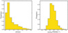 |
Fig. 1 Observing conditions under which the data released in DR1 were obtained. Top panel: airmass of individual exposures, which is mostly constrained to below 1.5; bottom panel: seeing, measured directly on the spectra, which was mostly constrained to below 1′′. |
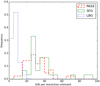 |
Fig. 2 Distribution of the median S/N per resolution element of all completed DR1 spectra, measured in the range 6000–7400 Å and separated for the three main VANDELS classes. The red dashed histogram refers to PASS galaxies, the blue dotted histogram to LBGs, and the green histogram to SFGs. Each histogram is normalized separately. |
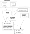 |
Fig. 3 Flow diagram illustrating the various steps of the data reduction pipeline. |
5 Redshift measurement
Spectroscopic redshifts and associated quality flags were determined for all objects using the Pandora software package, within the Easy-Z environment (Garilli et al. 2010). This software was used successfully in previous VIMOS surveys and can simultaneously display the 1D extracted spectrum, the 2D linearly resampled spectrum, the 1D sky spectrum, and the noise. It is also possible to inspect the image thumbnail of the object with the exact position of the slit, to determine whether other sources are visible in the same slit and the pixels over which the source was extracted. The core algorithm for redshift determination is the correlation with available galaxy spectral templates. A key element for the cross-correlation engine to deliver a robust measurement is the availability of reference templates that cover a wide range of galaxy and star types and a wide range of rest-frame wavelengths. To determine the VANDELS spectroscopic redshifts, we adopted templates derived from previous VIMOS observations for the VVDS (Le Fèvre et al. 2013) and zCOSMOS surveys (Lilly et al. 2007), with and withoutLyα emission. Alternatively, it is also possible to determine the redshift by manually estimating the center of one or more emission and aborption lines. In several cases, it was necessary to manually perform some cleaning of the spectra, that is, to remove obvious noise residuals at the location of strong sky lines, or the zero-order projection.
Each target was assigned to two measurers from the VANDELS team who independently determined the redshift and located the main spectral features (in emission or absorption). Each measurer also assigned a spectroscopic quality flag to the target: these quality flags were allocated according to the original system devised for the VVDS and are related to the confidence of the spectral measurement. The reliability flag may take the following values:
- 0:
no redshift could be assigned (redshift is set to Nan).
- 1:
50% probability to be correct. Some low S/N lines are identified, but there is a weak to moderate match with templates.
- 2:
70–80% probability to be correct. There are several matching absoption lines and a general good match with templates.
- 3:
95–100% probability to be correct. The spectrum shows multiple strong absorption and/or emission lines, giving a consistent redshift, and it has a moderate S/N. The cross-correlation signal is strong and matches the templates excellently well.
- 4:
100% probability to be correct. The spectrum shows multiple strong absorption and/or emission lines, giving a consistent redshift, and it has a high S/N. The cross-correlation signal is strong, and the continuum match to the templates is excellent.
- 9:
spectrum with a single emission line. The listed redshift is the most probable given the observed continuum and the shape of the emission line, and it has a >80% probability to be correct.
We emphasize that the quality flag only reflects the accuracy of the redshift determination and is in principle not related to the S/N of the spectrum, although almost all the QF = 4 spectra havea very high S/N. The quality flags for AGN spectra are preceded by a leading 1 (e.g., 12 or 14), the quality flags for spectra thatwere not primary targets (i.e., were serendipitously observed in a certain slit) are preceded by an additional 2; finally, the quality flags for spectra deemed to be problematic are preceded by an additional –1. In DR1, only the AGN flags are present, since the secondary targets will be released only at the end of the survey. Following their independent redshift determinations, the two measurers were required to compare their redshifts and flags and to reconcile any differences. As a final step, all spectra were also independently re-checked by the two PIs, and any remaining discrepancies in the redshifts and quality flagswere again reconciled. This final pass was especially necessary to homogenize the quality flags as much as possible, given the different expertise and ability of the various redshift measurers. Based on repeated measurements, the typical accuracy of the spectroscopic redshift measurements is estimated to be +/–0.0005 (~ 150 km s−1).
Forty-two objects in DR1 have a previously published spectroscopic redshift. These were included in the survey since the expected integration time (mostly 80 or 40 h) would result in spectra with a much higher S/N than for those available before. Of these 42 sources, one has no redshift assigned in VANDELS (but it is a source with half of the final scheduled integration) and one (AGN type) has a discrepant redshift, 3.442, with flag 1 in VANDELS and 2.448 from Trump et al. (2013), also with a low quality flag, indicating that the redshift was based on the match with the photometric redshift. For the other 40 objects, including all quality flags both for VANDELS redshifts and for the previous redshifts, Δ z = (zVANDELS − zold)∕(1 + zVANDELS) has a mean value of –0.0003 and an rms of 0.0016, slightly higher than the redshift uncertainty quoted above.
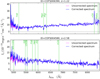 |
Fig. 4 Effect of the blue flux correction: in blue, we show the final corrected spectrum, and in magenta, we plot the original flux-calibrated spectrum for CDFS006390 at z = 1.22 (top panel), which was selected in the PASS sample, and CDFS004580 at z = 2.58, which was selected in the SFG sample. We also indicate with green vertical lines the main spectral features we identified. |
Detailed entry list in the catalogs associated with DR 1.
6 VANDELS DR1-data
Data release1 is available in the ESO archive and consists of all spectra obtained during the first VANDELS observing season, which ran from August 2015 until February 2016. The data were acquired during runs 194.A-2003(E-K). The data release includes the spectra for all galaxies for which the final scheduled integration time was completed during season 1 (356 objects, including 6 that received more than the scheduled time). In addition, DR1 also includes the spectra for 523 galaxies for which the scheduled integration time was 50% complete at the end of season 1 (i.e., 20 out of 40 scheduled hours and 40 out of 80 scheduled hours). The total number of spectra released is 879 (415 in CDFS and 464 in UDS).
For each target the following data files are being released:
- 1)
1D spectrum in FITS format, containing the following arrays: WAVE: wavelength in Angstroms (in air); FLUX: 1D spectrum blue-corrected flux in erg cm−2 s−1 Angstrom−1; ERR: noise estimate in erg cm−2 s−1 Angstrom−1; UNCORR-FLUX: 1D spectrum flux uncorrected for blue flux loss (see details in Sect. 4); SKY: the subtracted sky in counts.
- 2)
2D resampled and sky-subtracted (but not flux-calibrated, nor corrected for atmospheric extinction) spectrum in FITS format.
- 3)
Catalog with essential galaxy parameters, listed in Table 1 and presented in Table 2, which include iAB, zAB, and HAB magnitudes with the relevant filters (see below), the scheduled and current integration times, and the spectroscopic redshift and quality flag determined as in Sect. 5. As described in Sect. 2, the UDS and CDFS fields are covered by different observation sets, with 45% of the area covered by deep HST imaging (the CANDELS footprint) and the rest covered only by ground-based imaging (the wider surrounding areas). For this reason, the iAB, zAB, and HAB magnitudes listed in the release catalogs are generated from different filters. For each object, the origin of the iAB, zAB, and HAB photometry is listed in the catalog in the columns with the filter name. Here we list the match between the catalog photometry and the filters used.
iAB magnitudes refer to the SUBARU i′-filter for the UDS-GROUND and UDS-HST targets, to the F775W filter for CDFS-HST targets, and to the SUBARU IA738 filter for the CDFS-GROUND targets.
zAB magnitudes refer to the SUBARU z′-filter for the UDS-GROUND and UDS-HST targets and to the F850LP filter for the CDFS-GROUND and CDFS-HST targets.
HAB magnitudes refer to the F160W filter for the UDS-HST and CDFS-HST targets, the WFCAM H-filter for the UDS-GROUND targets, and the VISTA H-filter for the CDFS-GROUND targets.
In the catalog we report both the total requested integration time (tschedtime) and the current total integration time (texptime). Clearly, theobjects for which the observations are not completed will have texptime < tschedtime. In some cases, objects have texptime > tschedtime. The reason for this is that because of changing observing conditions, some masks in both the UDS and CDFS fields have received slightly more than their nominally scheduled 20 h of on-source integration. In addition, to optimize slit allocation, six objects in this data release that required 20 h of on-source integration were placed on two VIMOS masks and therefore received 40 h of on-source integration.
In Fig. 5, we present the redshift distribution of all DR1 spectra, separated by the original target classification (i.e., the AGN class includes the targets originally selected as AGN and not the flag 14 objects). The quality flag statistics for galaxies in DR1 are reported in Table 3 and are as follows: 299 galaxies, 34% of the sample, received a flag 4 or 14; 184 galaxies, 21%, received a flag 3; 156 galaxies, 18%, received a flag 2; 180 galaxies, 20%, received a flag 1; and 54 galaxies, 6%, received a flag 9. For 6 objects no redshift was assigned, and they are therefore labeled as flag 0. The same tabl also shows that in the two main classes of targets (SFG and PASS), the large majority of galaxies has flag ≥ 3, while AGN- and Herschel-selected sources all have lower quality flags. Four targets have a flag 14, indicating that their spectra show AGN features. Only one of them was originally selected as AGN, while 2 were selected as LBGs and 1 as SFG. In the other selected AGN, no prominent AGN features were identified even when the redshift was determined.
Data release 1 catalog: random examples of galaxies.
7 Galaxies in DR1
7.1 General properties and redshift distribution
The targets in DR1 belong to the following category: 177 objects are selected as SFG with 2.4 < zphot < 5.5, 106 objects are PASS with 1.0 < zphot < 2.5, 566 objects are LBG with 3.0 < zphot < 5.5, and 6 are LBG with 5.5 < zphot < 7.0. In addition, 18 targets were selected as radio or X-ray AGN (all in the CDFS field), and 6 are Herschel-selected sources (3 in each field). These numbers, with the subdivision into fields, are reported in Table 4.
7.2 Photometric redshift accuracy
In Figs. A.1 and A.2, we show the plots of the photometric redshifts versus spectroscopic redshifts for all galaxies that are part of the DR1 set for which a redshift could be determined (873 objects), separated by flag type and target category. We also show in Fig. A.3 the same plot for objects thatreceived the full final integration time (20, 40, or 80 h) and those that received only half of the final allocation.
In Table 5, we report the number of outliers and the resulting scatter between the photometric redshifts and the spectroscopic redshifts, where the photometric redshift is that of CANDELS for the CANDELS footprint areas, and that of VANDELS (McLure et al. 2018) for the outer areas. This table presents both the full scatter σF = rms(Δz) where Δ z = (zspec − zphot)∕(1 + zspec), and σO derived after excluding the catastrophic outliers. We define a catastrophic outlier as a galaxy for which |Δ z| > 0.15. We remark that σO gives a non-optimal representation of the scatter since a few objects (i.e., the outliers) can drive the scatter to high values. We also quantify any systematic bias between photometric and spectroscopic redshifts by b = mean(Δz) after excluding the outliers. The table shows that the bias is much lower than the scatter.
There are 18 outliers, which means that the resulting rate is 2.1%. This perfectly agrees with the rate estimated based on the accuracy of the VANDELS photometric redshifts, even though they have been validated on a sample with brighter average magnitude (see McLure et al. 2018 for details). The number of outliers is higher for flag 1 and 9 objects, as expected, while it is extremely low for flags 2–4. This indicates that our flag system is conservative and the flags probably underestimate the reliability of the redshift. We note that 8 of the 18 outliers are AGN- or Herschel-selected sources. In particular, for AGN, the disagreement between photometric and spectroscopic redshift might arise partly because only templates of normal galaxies were used to determine the photometric redshifts (Salvato et al. 2011, 2009).
If we further restrict the sample to the three main target categories of the VANDELS proposal, the outliers rate is only 1.2%, which is extremely low. The table shows that the agreement between zphot and zspec is excellent for all quality flags with σO, clearly improving for higher flags. The class of targets with the highest overall accuracy is PASS: this is easily explained by the relative brightness of this sample (the median H-band magnitude is H = 21.4) and by very clear break in the SED of the 4000 Å break for galaxies in this redshift range. In the same table we report the accuracy of the photometric redshifts divided by H-magnitude bins after removing the Herschel and AGN targets for an unbiased view of the three main VANDELS groups. We find that σo decreases mildly as a function of the H-band magnitude, while the percentage of outliers slightly increases at fainter magnitudes. This was also found by Dahlen et al. (2013) for the CANDELS photometric redshifts, although in that case, the fraction of outliers at magnitude fainter than 25 was much higher, > 10%, compared to our 2.3% even in the faintest bin. We also investigate the photometric redshift accuracy as a function of redshift, again after removing the Herschel and AGN targets. Figure 6 indicates a redshift trend in the photometric redshift accuracy, since the scatter σo increases very smoothly from σo = 0.016 at z~ 1−1.3 to σo = 0.044 at z~ 3.5−4 and beyond this redshift, it decreases.
We finally compare the accuracy of photometric redshifts in the CANDELS footprint and in the outer areas. The largest number of outliers is found in the CANDELS areas (16), but the main reason is that all the Herschel targets and almost all of the AGN (i.e., the classes with the majority of interlopers) are selected in the CANDELS areas, and the CANDELS targets are also on average 0.4 magnitudes fainter than those in the wider areas. However, the new VANDELS redshifts (i.e., those in the outer areas) also have a lower bias and scatter. A possible explanation for the increased success rate of the VANDELS photometric redshifts is that all potential targets were visually inspected before the final assembly of the catalog to reject obviously spurious detections and artifacts. Similar results on the accuracy of photometric redshifts were recently obtained by Masters et al. (2017) from the Calibration of the Color–Redshift Relation (C3R2) survey that was carried out with the Keck telescope.
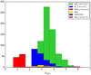 |
Fig. 5 Spectroscopic redshift distribution of all DR1 targets, divided by the original target classification. |
Galaxies in DR1 divided by flag.
Galaxies in DR1 divided by target type.
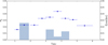 |
Fig. 6 Redshift dependence of the photometric redshift scatter and outlier fraction from a comparison of photometric and spectroscopic redshift. The blue dots show the scatter σO (scaling on left-hand y-axis). The histograms show the fraction of outliers (scaling on right-hand y-axis). The sample does not include Herschel and AGN selected targets. |
Accuracy of photometric redshifts.
7.3 Examples of data products
To illustrate the content of the VANDELS-DR1, we present some examples of data products for different types of targets and different quality flag. Figures 7–10 show the 2D and 1D sky and noise spectra of four targets, selected as PASS, LBG, SFG, and AGN, respectively. All these galaxies have quality flags 4, since the redshift is determined with great accuracy from the many emission and or/absorption lines visible in the spectra. To illustrate the meaning of the different quality flags, we present in Fig. 11 the spectra of five galaxies, all selected as LBGs, and approximately at the same redshift (z ~ 4), but with quality flags 4, 3, 2, 1, and 9, respectively. In the spectrum with flag 4, two emission lines (the Lyα and HeII lines) and several absorption lines such as the SiII, OI, CII, and CIV can clearly be identified. The drop in the continuum flux below the Lyα line is also very clear. In the spectrum with flag 3 spectrum, the Lyα and several absorption lines (e.g., the SiII and CIV) are identified, together with the drop in the continuum flux. The spectrum with flag 2 (which is smoothed in the figure for clarity) shows the SiII, CII and SiIV lines with good confidence, and the drop in the continuum flux is also clear. The spectrum with flag 1 shows only the SiIV line clearly, but the agreement is good in general when we cross-correlate this spectrum with templates at the assigned redshift. Finally, the flag 9 case shows only one bright emission line in the spectrum. The line does not show a prominent asymmetry (which would clearly identify it as Lyα), and no continuum is detected blueward of the line, therefore, some ambiguity remains in the redshift identification.
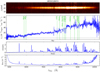 |
Fig. 7 From top to bottom: 2D spectrum, 1D extracted spectrum, sky counts, and rms noise of target VANDELS-UDS-018651. This object was selected as a PASS galaxy and has a redshift 1.093 with flag 4. The main spectral features are indicated in the 1D spectrum. |
8 Summary
We have presented the first data release of the VANDELS public spectroscopic survey. VANDELS, a deep survey of the CANDELS CDFS and UDS fields, is an ESO public survey carried out with VIMOS and has obtained more than 2000 ultra-deep medium-resolution spectra of galaxies in the wavelength range 4800–10 000 Å. DR1 is the release of all spectra obtained during the first season of observations, and it includes all targets for which either the scheduled integration time or half of the total time was completed. The release includes spectra for 879 objects, 464 in the UDS and 415 in the CDFS. Together with the spectra, we release the spectroscopic redshifts measured by the collaboration, with a quality flag that assesses their reliability. We here presented the statistics of the redshift quality and discussed the excellent accuracy of the VANDELS photometric redshifts, with an outlier rate as low as 2.1% and an overall accuracy of σo = 0.035, which improves when we restrict the statistics to the main VANDELS target categories. We also presented some examples of data products to illustrate the content of the release. All spectra and information are available in the ESO archive. The second data release will include all spectra that are completed during the second observational season, and will be available in September 2018. A final release is expected for June 2020 and will include an improved re-reduction of the entire spectroscopic data, a series of galaxy physical properties (stellar masses, SFRs, dust attenuation, etc.) derived by the collaboration through SED fitting, and measurements of absorption and emission lines that we identified in the VANDELS spectra.
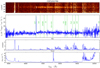 |
Fig. 8 From top to bottom: 2D spectrum, 1D extracted spectrum, sky counts, and rms noise of target VANDELS-CDFS-202794. This object has an H-band magnitude of 24.1 and was selected in the category LBG. It was assigned a zspec = 4.4266 and flag 4. The main spectral features (emission lines and interstellar absorption lines) are indicated in the 1D spectrum. |
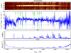 |
Fig. 9 From top to bottom: 2D spectrum, 1D extracted spectrum, sky counts, and rms noise of target VANDELS-UDS-003664. This object has an H-band magnitude of 23.1 and was selected in the category SFG. It was assigned a zspec = 3.703 and Flag 4. The main spectral features (the Lyα absorption and several interstellar absorption lines) are indicated in the 1D spectrum. |
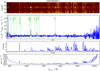 |
Fig. 10 From top to bottom: 2D spectrum, 1D extracted spectrum, sky counts, and rms noise of target VANDELS-CDFS-005827. This object was selected as an AGN target and is indeed identified as an AGN (quality flag 14) at z = 3.0328. The main spectral features (the Lyα, CIV, HeII, and CIII] emission lines) are indicated in the 1D spectrum. |
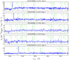 |
Fig. 11 From top to bottom: 1D extracted spectra of five VANDELS LBGs at redshift z ~ 4 with different quality flags: VANDES-CDFS-226606 with QF = 4, VANDELS-UDS-012992 with QF = 3, VANDELS-UDS-384986 with QF = 2, VANDELS-UDS-305866 with QF = 1, and VANDELS-CDFS-029443 with QF = 9. The spectra of the QF = 1 and 2 galaxies have been slightly smoothed to show the absorption lines better. |
Acknowledgement
Based on data products from observations made with ESO Telescopes at the La Silla Paranal Observatory under program ID 194.A-2003(E-K). We thank the ESO staff for their continuous support for the VANDELS survey, particularly the Paranal staff, who helped us to conduct the observations, and the ESO user support group in Garching. R.J.M, A.M., E.M.Q., and D.J.M. acknowledge funding from the European Research Council via the award Consolidator Grant (P.I. R. McLure). A.C. acknowledges grant PRIN-MIUR 2015 and ASI n.I/023/12/0. P.C. acknowledges support from CONICYT through the project FONDECYT regular 1150216. R.M. acknowledges support by ERC Advanced Grant 695671 “QUENCH”. F.B. acknowledges support by Fundação para a Ciência e a Tecnologia (FCT) via the postdoctoral fellowship SFRH/BPD/103958/2014 and through research grant UID/FIS/04434/2013.
Appendix A Additional figures
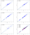 |
Fig. A.1 zphot vs. zspec for all galaxies in DR1, separated by flag type. The galaxies falling outside the dashed lines are the catastrophic outliers that have |dz| > 0.15. |
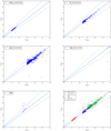 |
Fig. A.2 zphot vs. zspec for all galaxies separated by selection class type. The galaxies falling outside the dashed lines are the catastrophic outliers that have |dz| > 0.15. |
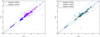 |
Fig. A.3 zphot vs. zspec for all galaxies, color-coded by integration time. We show at the left the galaxies that received half of the final integration time, and at the right the galaxies that received the full (20, 40, or 80 h) integration time. The galaxies falling outside the dashed lines are the catastrophic outliers that have |dz| > 0.15. |
Appendix B Glossary
We list here some of the acronyms used in the paper:
CANDELS: Cosmic Assembly Near-infrared Deep Extragalactic Survey
CDFS: Chandra Deep Field South
GMASS: Galaxy Mass Assembly ultra-deep Spectroscopic Survey
KBSS: KeckBaryonic Structure Survey
SPOC: Slit Positioning Optimization Code
UDS: Ultra Deep Survey
VIMOS: VIsible MultiObject Spectrograph
VIPERS: VIMOS Public Extragalactic Redshift Survey
VMMPS: VIMOS Mask Preparation Software
VUDS: VIMOS Ultra Deep Survey
VVDS: VIMOS VLT Deep Survey
References
- Alam, S., Albareti, F. D., Allende Prieto, C., et al. 2015, ApJS, 219, 12 [NASA ADS] [CrossRef] [Google Scholar]
- Bottini, D., Garilli, B., Maccagni, D., et al. 2005, PASP, 117, 996 [NASA ADS] [CrossRef] [Google Scholar]
- Chang, Y.-Y., Le Floc’h, E., Juneau, S., et al. 2017, ApJS, 233, 19 [NASA ADS] [CrossRef] [Google Scholar]
- Cimatti, A., Cassata, P., Pozzetti, L., et al. 2008, A&A, 482, 21 [NASA ADS] [CrossRef] [EDP Sciences] [Google Scholar]
- Dahlen, T., Mobasher, B., Faber, S. M., et al. 2013, ApJ, 775, 93 [Google Scholar]
- De Barros, S., Pentericci, L., Vanzella, E., et al. 2017, A&A, 608, A123 [NASA ADS] [CrossRef] [EDP Sciences] [Google Scholar]
- Ellis, R. S., Bland-Hawthorn, J., Bremer, M., et al. 2017, ArXiv e-prints [arXiv:1701.01976] [Google Scholar]
- Galametz, A., Grazian, A., Fontana, A., et al. 2013, ApJS, 206, 10 [NASA ADS] [CrossRef] [Google Scholar]
- Garilli, B., Fumana, M., Franzetti, P., et al. 2010, PASP, 122, 827 [NASA ADS] [CrossRef] [Google Scholar]
- Grogin, N. A., Kocevski, D. D., Faber, S. M., et al. 2011, ApJS, 197, 35 [NASA ADS] [CrossRef] [Google Scholar]
- Guo, Y., Ferguson, H. C., Giavalisco, M., et al. 2013, ApJS, 207, 24 [NASA ADS] [CrossRef] [Google Scholar]
- Guzzo, L., Scodeggio, M., Garilli, B., et al. 2014, A&A, 566, A108 [NASA ADS] [CrossRef] [EDP Sciences] [Google Scholar]
- Horne, K. 1986, PASP, 98, 609 [NASA ADS] [CrossRef] [EDP Sciences] [Google Scholar]
- Hsu, L.-T., Salvato, M., Nandra, K., et al. 2014, ApJ, 796, 60 [NASA ADS] [CrossRef] [Google Scholar]
- Koekemoer, A. M., Faber, S. M., Ferguson, H. C., et al. 2011, ApJS, 197, 36 [NASA ADS] [CrossRef] [Google Scholar]
- Kurk, J., Cimatti, A., Daddi, E., et al. 2013, A&A, 549, A63 [NASA ADS] [CrossRef] [EDP Sciences] [Google Scholar]
- Le Fèvre, O., Saisse, M., Mancini, D., et al. 2003, Proc. SPIE, 4841, 1670 [NASA ADS] [CrossRef] [Google Scholar]
- Le Fèvre, O., Vettolani, G., Garilli, B., et al. 2005, A&A, 439, 845 [NASA ADS] [CrossRef] [EDP Sciences] [Google Scholar]
- Le Fèvre, O., Cassata, P., Cucciati, O., et al. 2013, A&A, 559, A14 [NASA ADS] [CrossRef] [EDP Sciences] [Google Scholar]
- Le Fèvre, O., Tasca, L. A. M., Cassata, P., et al. 2015, A&A, 576, A79 [NASA ADS] [CrossRef] [EDP Sciences] [Google Scholar]
- Lilly, S. J., Le Fèvre, O., Renzini, A., et al. 2007, ApJS, 172, 70 [NASA ADS] [CrossRef] [Google Scholar]
- Masters, D. C., Stern, D. K., Cohen, J. G., et al. 2017, ApJ, 841, 111 [NASA ADS] [CrossRef] [Google Scholar]
- McLure, R. J., Pentericci, L., Cimatti, A., et al. 2018, MNRAS, 479, 25 [NASA ADS] [Google Scholar]
- Oke, J. B., & Gunn, J. E. 1983, ApJ, 266, 713 [NASA ADS] [CrossRef] [Google Scholar]
- Pentericci, L., Vanzella, E., Castellano, M., et al. 2018, A&A, in press, DOI: 10.1051/0004-6361/201732465 [Google Scholar]
- Reid, B., Ho, S., Padmanabhan, N., et al. 2016, MNRAS, 455, 1553 [NASA ADS] [CrossRef] [Google Scholar]
- Rix, H.-W., Barden, M., Beckwith, S. V. W., et al. 2004, ApJS, 152, 163 [NASA ADS] [CrossRef] [Google Scholar]
- Salvato, M., Hasinger, G., Ilbert, O., et al. 2009, ApJ, 690, 1250 [CrossRef] [Google Scholar]
- Salvato, M., Ilbert, O., Hasinger, G., et al. 2011, ApJ, 742, 61 [NASA ADS] [CrossRef] [Google Scholar]
- Santini, P., Ferguson, H. C., Fontana, A., et al. 2015, ApJ, 801, 97 [NASA ADS] [CrossRef] [Google Scholar]
- Scodeggio, M., Franzetti, P., Garilli, B., et al. 2005, PASP, 117, 1284 [NASA ADS] [CrossRef] [Google Scholar]
- Shibuya, T., Ouchi, M., Konno, A., et al. 2018, PASJ, 70, S14 [Google Scholar]
- Sommariva, V., Mannucci, F., Cresci, G., et al. 2012, A&A, 539, A136 [NASA ADS] [CrossRef] [EDP Sciences] [Google Scholar]
- Steidel, C. C., Rudie, G. C., Strom, A. L., et al. 2014, ApJ, 795, 165 [NASA ADS] [CrossRef] [Google Scholar]
- Trump, J. R., Konidaris, N. P., Barro, G., et al. 2013, ApJ, 763, L6 [Google Scholar]
- Williams, R. J., Quadri, R. F., Franx, M., van Dokkum, P., & Labbé, I. 2009, ApJ, 691, 1879 [NASA ADS] [CrossRef] [Google Scholar]
- Xue, Y. Q., Luo, B., Brandt, W. N., et al. 2011, ApJS, 195, 10 [NASA ADS] [CrossRef] [Google Scholar]
All Tables
All Figures
|
Fig. 1 Observing conditions under which the data released in DR1 were obtained. Top panel: airmass of individual exposures, which is mostly constrained to below 1.5; bottom panel: seeing, measured directly on the spectra, which was mostly constrained to below 1′′. |
| In the text | |
|
Fig. 2 Distribution of the median S/N per resolution element of all completed DR1 spectra, measured in the range 6000–7400 Å and separated for the three main VANDELS classes. The red dashed histogram refers to PASS galaxies, the blue dotted histogram to LBGs, and the green histogram to SFGs. Each histogram is normalized separately. |
| In the text | |
|
Fig. 3 Flow diagram illustrating the various steps of the data reduction pipeline. |
| In the text | |
|
Fig. 4 Effect of the blue flux correction: in blue, we show the final corrected spectrum, and in magenta, we plot the original flux-calibrated spectrum for CDFS006390 at z = 1.22 (top panel), which was selected in the PASS sample, and CDFS004580 at z = 2.58, which was selected in the SFG sample. We also indicate with green vertical lines the main spectral features we identified. |
| In the text | |
|
Fig. 5 Spectroscopic redshift distribution of all DR1 targets, divided by the original target classification. |
| In the text | |
|
Fig. 6 Redshift dependence of the photometric redshift scatter and outlier fraction from a comparison of photometric and spectroscopic redshift. The blue dots show the scatter σO (scaling on left-hand y-axis). The histograms show the fraction of outliers (scaling on right-hand y-axis). The sample does not include Herschel and AGN selected targets. |
| In the text | |
|
Fig. 7 From top to bottom: 2D spectrum, 1D extracted spectrum, sky counts, and rms noise of target VANDELS-UDS-018651. This object was selected as a PASS galaxy and has a redshift 1.093 with flag 4. The main spectral features are indicated in the 1D spectrum. |
| In the text | |
|
Fig. 8 From top to bottom: 2D spectrum, 1D extracted spectrum, sky counts, and rms noise of target VANDELS-CDFS-202794. This object has an H-band magnitude of 24.1 and was selected in the category LBG. It was assigned a zspec = 4.4266 and flag 4. The main spectral features (emission lines and interstellar absorption lines) are indicated in the 1D spectrum. |
| In the text | |
|
Fig. 9 From top to bottom: 2D spectrum, 1D extracted spectrum, sky counts, and rms noise of target VANDELS-UDS-003664. This object has an H-band magnitude of 23.1 and was selected in the category SFG. It was assigned a zspec = 3.703 and Flag 4. The main spectral features (the Lyα absorption and several interstellar absorption lines) are indicated in the 1D spectrum. |
| In the text | |
|
Fig. 10 From top to bottom: 2D spectrum, 1D extracted spectrum, sky counts, and rms noise of target VANDELS-CDFS-005827. This object was selected as an AGN target and is indeed identified as an AGN (quality flag 14) at z = 3.0328. The main spectral features (the Lyα, CIV, HeII, and CIII] emission lines) are indicated in the 1D spectrum. |
| In the text | |
|
Fig. 11 From top to bottom: 1D extracted spectra of five VANDELS LBGs at redshift z ~ 4 with different quality flags: VANDES-CDFS-226606 with QF = 4, VANDELS-UDS-012992 with QF = 3, VANDELS-UDS-384986 with QF = 2, VANDELS-UDS-305866 with QF = 1, and VANDELS-CDFS-029443 with QF = 9. The spectra of the QF = 1 and 2 galaxies have been slightly smoothed to show the absorption lines better. |
| In the text | |
|
Fig. A.1 zphot vs. zspec for all galaxies in DR1, separated by flag type. The galaxies falling outside the dashed lines are the catastrophic outliers that have |dz| > 0.15. |
| In the text | |
|
Fig. A.2 zphot vs. zspec for all galaxies separated by selection class type. The galaxies falling outside the dashed lines are the catastrophic outliers that have |dz| > 0.15. |
| In the text | |
|
Fig. A.3 zphot vs. zspec for all galaxies, color-coded by integration time. We show at the left the galaxies that received half of the final integration time, and at the right the galaxies that received the full (20, 40, or 80 h) integration time. The galaxies falling outside the dashed lines are the catastrophic outliers that have |dz| > 0.15. |
| In the text | |
Current usage metrics show cumulative count of Article Views (full-text article views including HTML views, PDF and ePub downloads, according to the available data) and Abstracts Views on Vision4Press platform.
Data correspond to usage on the plateform after 2015. The current usage metrics is available 48-96 hours after online publication and is updated daily on week days.
Initial download of the metrics may take a while.