| Issue |
A&A
Volume 616, August 2018
|
|
|---|---|---|
| Article Number | A27 | |
| Number of page(s) | 13 | |
| Section | Numerical methods and codes | |
| DOI | https://doi.org/10.1051/0004-6361/201832858 | |
| Published online | 07 August 2018 | |
Image Domain Gridding: a fast method for convolutional resampling of visibilities
Netherlands Institute for Radio Astronomy (ASTRON),
Postbus 2,
7990
AA Dwingeloo,
The Netherlands
e-mail: This email address is being protected from spambots. You need JavaScript enabled to view it.
Received:
20
February
2018
Accepted:
21
March
2018
Abstract
In radio astronomy obtaining a high dynamic range in synthesis imaging of wide fields requires a correction for time and direction-dependent effects. Applying direction-dependent correction can be done by either partitioning the image in facets and applying a direction-independent correction per facet, or by including the correction in the gridding kernel (AW-projection).
An advantage of AW-projection over faceting is that the effectively applied beam is a sinc interpolation of the sampled beam, where the correction applied in the faceting approach is a discontinuous piece wise constant beam. However, AW-projection quickly becomes prohibitively expensive when the corrections vary over short time scales. This occurs, for example, when ionospheric effects are included in the correction. The cost of the frequent recomputation of the oversampled convolution kernels then dominates the total cost of gridding.
Image domain gridding is a new approach that avoids the costly step of computing oversampled convolution kernels. Instead low-resolution images are made directly for small groups of visibilities which are then transformed and added to the large uv grid. The computations have a simple, highly parallel structure that maps very well onto massively parallel hardware such as graphical processing units (GPUs). Despite being more expensive in pure computation count, the throughput is comparable to classical W-projection. The accuracy is close to classical gridding with a continuous convolution kernel. Compared to gridding methods that use a sampled convolution function, the new method is more accurate. Hence, the new method is at least as fast and accurate as classical W-projection, while allowing for the correction for quickly varying direction-dependent effects.
Key words: instrumentation: interferometers / methods: numerical / techniques: image processing
© ESO 2018
1 Introduction
In aperture synthesis radio astronomy an image of the sky brightness distribution is reconstructed from measured visibilities. A visibility is the correlation coefficient between the electric field at two different locations. The relationship between the sky brightness distribution and the expected visibilities is a linear equation commonly referred to as the measurement equation (ME; Smirnov 2011).
An image could be reconstructed using generic solving techniques, but the computational cost of any reasonably sized problem is prohibitively large. The cost can be greatly reduced by using the fact that under certain conditions the ME can be approximated by a two-dimensional (2D) Fourier transform. The discretized version of the ME can then be evaluated using the very efficient fast Fourier transform (FFT).
To use the FFT, the data need to be on a regular grid. Since the measurements have continuous coordinates, they first need to be resampled onto a regular grid. In Brouw (1975), a convolutional resampling method is introduced known as “gridding”. The reverse step, needed to compute model visibilities on continuous coordinates from a discrete model, is known as degridding.
For larger fields of view the approximation of the ME by a Fourier transform is inaccurate. The reduction of the full three-dimensional (3D) description to two dimensions only holds when all antennas are in a plane that is parallel to the image plane. Also, the variations of the instrumental and atmospheric effects over the field of view are not included.
There are two approaches to the problem of wide field imaging: (1) Partition the image into smaller sub-images or facets such that the approximations hold for each of the facets. The facets are then combined together whereby special care needs to be taken to avoid edge effects (Cornwell & Perley 1992; Tasse et al. 2018); and (2) include deviations from the Fourier transform in the convolution function. The W-projection algorithm (Cornwell et al. 2005) includes the non-coplanar baseline effect. The A-projection algorithm (Bhatnagar et al. 2008) extended upon this by also including instrumental effects. For the Low-Frequency Array (LOFAR), it is necessary to include ionospheric effects as well (Tasse et al. 2013). Each successive refinement requires the computation of more convolution kernels. The computation of the kernels can dominate the total cost of gridding, especially when atmospheric effects are included in the convolution kernel, because these effects can vary over short time scales.
The high cost of computing the convolution kernels is the main motivation for the development of a new algorithm for gridding and degridding. The new algorithm presented in this paper effectively performs the same operation as classical gridding and degridding with AW-projection, except that it does this more efficiently by avoiding the computation of convolution kernels altogether. Unlike, for example, the approach by Young et al. (2015), the corrections do not need to be decomposable in a small number of basis functions.
The performance in terms of speed of various implementations of the algorithm on different types of hardware is the subject of Veenboer et al. (2017). The focus of this paper is on the derivation of the algorithm and analysis of its accuracy.
The paper is structured as follows. In Sect. 2 we review the gridding method and AW-projection. In Sect. 3 we introduce the new algorithm which takes the gridding operation to the image domain. In Sect. 4 the optimal taper for the image domain gridding is derived. Image domain gridding with this taper results in a lower error than classical gridding with the classical optimal window. In Sect. 5 both the throughput and the accuracy are measured.
The following notation is used throughout the paper. Complex conjugation of x is denoted x*. Vectors are indicated by bold lower case symbols, for example, v, matrices by bold upper case symbols, M. The Hermitian transpose of a vector or matrix is denoted vH, MH, respectively.For continuous and discrete (sampled) representations of the same object, a single symbol is used. Where necessary, the discrete version is distinguished from the continuous one by a superscript indicating the size of the grid, that is, VL ×L is a grid of L × L pixels sampling continuous function V. Square brackets are used to address pixels in a discrete grid, for example, V [i, j], while parentheses are used for the value at continuous coordinates, V (u, v). A convolution is denoted by *; the (discrete) circular convolution by ⊛. The Fourier transform, both continuous and discrete, is denoted by  . In algorithms we use ← for assignment.
A national patent (The Netherlands only) for the method presented in this paper has been registered at the European Patent Office in The Hague, The Netherlands (van der Tol 2017). No international patent application will be filed. Parts of the description of the method and corresponding figures are taken from the patent application. The software has been released (Veenboer 2017) under the GNU General Public License1. The GNU GPL grants a license to the patent for usage of this software and derivatives published under the GNU GPL. To obtain a license for uses other than under GPL, please contact Astron2.
2 Gridding
In this section we summarize the classical gridding method. The equations presented here are the starting point for the derivation of image domain gridding in the following section.
The output of the correlator of an aperture synthesis radio telescope is described by the ME (Smirnov 2011). The full polarization equation can be written as a series of 4 × 4 matrix products (Hamaker et al. 1996) or a series of 2 × 2 matrix products from two sides (Hamaker 2000). For convenience, but without loss of generality, the derivations in this paper are done for the scalar (non-polarized) version of the ME. The extension of the results in this paper to the polarized case is straightforward, by writing out the matrix multiplications in the polarized ME as sums of scalar multiplications.
The scalar equation for visibility yijqr for baseline i, j, channel q at timestep r is given by
 (1)
(1)
where I(l, m) is the brightness distribution or sky image, (uijr, vijr, wijr) is the baseline coordinate, and (l, m, n) is the direction coordinate, with  , λq is the wavelength for the qth channel, and giqr (l, m) is the complex gain pattern of the ith antenna. To simplify the notation, we lump indices i, j, q, r together into a single index k, freeing indices i, j, q, r for other purposes later on. Defining
 (2)
(2)
allows us to write Eq. (1) as
 (3)
(3)
The observed visibilities ŷk are modeled as the sum of a model visibility yk and noise ηk:
 (4)
(4)
The noise ηk is assumed to be Gaussian, have a mean of zero, and be independent for different k, with variance  .
.
Image reconstruction is finding an estimate of image I(l, m) from a set ofmeasurements {ŷk}. We loosely follow a previously published treatment of imaging (Cornwell et al. 2008; Appendix A). To reconstruct a digital image of the sky it is modeled as a collection of point sources. The brightness of the point source at (li, mj) is given by the value of the corresponding pixel I[i, j]. The source positions li, mj are given by
 (5)
(5)
where L is the size of one side of the imagein pixels, and S the size of the image projected onto the tangent plane.
Discretization of the image leads to a discrete version of the ME, or DME:
![Mathematical equation: \begin{equation*} y_k = \sum_{i=1}^L\sum_{j=1}^L {\rm{e}}^{-j2\pi\left(u_k l_i + v_k m_j + w_k n'_{ij} \right)} g_k(l_i,m_j) I[i,j].\end{equation*}](/articles/aa/full_html/2018/08/aa32858-18/aa32858-18-eq9.png) (6)
(6)
This equation can be written more compactly in matrix form, by stacking the pixels I[i, j] in a vector x, the visibilities yk in a vector y, and collecting the coefficients  in a matrix A:
 (7)
(7)
The vector of observed visibilities  is the sum of the vector of model visibilities y and the noise vector η. Because the noise is Gaussian, the optimally reconstructed image
  is a least squares fit to the observed data
  :
:
 (8)
(8)
where Σ is the noise covariance matrix, assumed to be diagonal, with  on the diagonal. The solution is well known and given by
 (9)
(9)
In practice, the matrices are too large to directly evaluate this equation. Even if it could be computed, the result would be of poor quality, because matrix AHΣA is usually ill-conditioned. Direct inversion is avoided by reconstructing the image in an iterative manner. Additional constraints and/or a regularization are applied, either explicitly or implicitly.
Most, if not all, of these iterative procedures need the derivative of cost function (8) to compute the update. This derivative is given by
 (10)
(10)
In this equation, the product Ax can be interpreted as the model visibilities y for model image x. The difference then becomes  , which can be interpreted as the residual visibilities. Finally, the multiplication of
  or
or  by AH Σ−1 computes the dirty, or residual image, respectively. This is equivalent to the Direct Imaging Equation (DIE), in literature often denoted by the misnomer3 Direct Fourier Tranform (DFT):
![Mathematical equation: \begin{equation*} \hat{I}[i,j] = \sum_{k=0}^{K-1} {\rm{e}}^{\mathrm{j}2\pi\left(u_k l_i + v_k m_j + w_k n'_{ij} \right)} g_k^*(l_i,m_j) \gamma_k \hat{y}_k,\end{equation*}](/articles/aa/full_html/2018/08/aa32858-18/aa32858-18-eq22.png) (11)
(11)
where γk is the weight. The weight can be set to  (the entries of the main diagonal of Σ−1) for natural weighting, minimizing the noise, but often other weighting schemes are used, making a trade off between noise and resolution. Evaluation of the equations above is still expensive. Because the ME is close to a Fourier transform, the equations can be evaluated far more efficiently by employing the FFT.
To use the FFT, the measurements need to be put on a regular grid by gridding. Gridding is a (re)sampling operation in the uv domain that causes aliasing in the image domain, and must therefore be preceded by a filtering operation. The filter is a multiplication by a taper c(l, m) in the image domain, suppressing everything outside the area to be imaged. This operation is equivalent to a convolution in the uv domain by C(u, v), the Fourier transform of the taper. Let the continuous representation of the observed visibilities after filtering be given by
 (12)
(12)
Now the gridded visibilities are given by
![Mathematical equation: \begin{equation*} \widehat{V}^{L \times L}[i,j] = \widetilde{V}(u_i, v_j) \quad \text{for } 0 \le i,j < L. \end{equation*}](/articles/aa/full_html/2018/08/aa32858-18/aa32858-18-eq25.png) (13)
(13)
The corresponding image is given by
 (14)
(14)
The divisionby cL×L in Eq. (14) is to undo the tapering of the image by the gridding kernel.
The degridding operation can be described by
 (15)
(15)
where Ck(u, v) is the gridding kernel and V (u, v) is the continuous representation of grid VL ×L:
![Mathematical equation: \begin{equation*} V(u,v) = \sum_{q=0}^{L}\sum_{r=0}^{L} \delta(u-u_r, v-v_r) V[q,r], \end{equation*}](/articles/aa/full_html/2018/08/aa32858-18/aa32858-18-eq28.png) (16)
(16)
Grid VL ×L is the discrete Fourier transform of model image IL ×L scaled by  :
:
 (17)
(17)
In this form, the reduction in computation cost by the transformation to the uv domain is not immediately apparent. However, the support of the gridding kernel is rather small, making the equations sparse, and hence cheap to evaluate. The kernel is the Fourier transform of the window function ck (l, m). In the simplest case, the window is a taper independent of time index k, ck (l, m) = b(l, m).
The convolution by the kernel in the uv domain applies a multiplication by the window in the image domain. This suppresses the side-lobes but also affects the main lobe. A well-behaved window goes towards zero near the edges. At the edges, the correction is unstable and that part of the image must be discarded. The image needs to be somewhat larger than the region of interest.
The cost of evaluating Eqs. (12) and (15) is determined by the support and the cost of evaluating Ck. The support is the size of the region for which Ck is non-negligible. Often Ck is precomputed on an over-sampled grid, because then only lookups are needed while gridding. In some cases Ck can be evaluated directly, but often only an expression in the image domain for ck is given. The convolution functions are then computed by evaluating the window functions on a grid that samples the combined image domain effect at least at the Nyquist rate, that is, the number of pixels M, must be at least as large as the support of the convolution function:
![Mathematical equation: \begin{equation*} c^{M\times M}[i,j] = c(l_i, m_j) \quad \text{for } 0 \leq i,j < M .\end{equation*}](/articles/aa/full_html/2018/08/aa32858-18/aa32858-18-eq31.png) (18)
(18)
This grid is then zero padded by the oversampling factor N to the number of pixels of the oversampled convolution function MN × MN:
 (19)
(19)
where li = −S∕(2M) + iS∕M, mj = −S∕(2M) + jS∕M, and  is the zero padding operator extending a grid to size MN × MN.
Since a convolution in the uv domain is a multiplication in the image domain, other effects that have the form of a multiplication in the image domain can be included in the gridding kernel as well.
2.1 W-projection
In Cornwell et al. (2005), W-projection is introduced. This method includes the effect of the non coplanar baselines in the convolution function. The corresponding window function is given by
 (20)
(20)
This correction depends on a single parameter only, the w coordinate. The convolution functions for a set of w values can be precomputed, and while gridding the nearest w coordinate is selected. The size of the W term can become very large which makes W projection expensive. The size of the W term can be reduced by either W-stacking (Humphreys & Cornwell 2011) or W-snapshots (Cornwell et al. 2012).
2.2 A-projection
A further refinement was introduced in Bhatnagar et al. (2008), to include the antenna beam as well:
 (21)
(21)
where gp(l, m) is the voltage reception pattern of the pth antenna.
As long as a convolution function is used to sample many visibilities, the relative cost of computing the convolution function is small. However, for low-frequency instruments with a wide field of view, both the A term and the W term vary over short time scales. The computation of the convolution kernels dominates over the actual gridding. The algorithm presented in the following section is designed to overcome this problem by circumventing the need to compute the kernels altogether.
3 Image domain gridding
In this section we present a new method for gridding and degridding. The method is derived from the continuous equations because the results follow more intuitively than in the discrete form. Discretization introduces some errors, but in the following section the accuracy of the algorithm is shown to be at least as good as classical gridding.
3.1 Gridding in the image domain
Computing the convolution kernels is expensive because they are oversampled. The kernels need to be oversampled because they need to be shifted to a continuous position in the uv domain. The key idea behind the new algorithm is to pull part of the gridding operation to the image domain, instead of transforming a zero-padded window function to the uv domain. In the image domain the continuous uv coordinate of a visibility can be represented by a phase gradient, even if the phase gradient is sampled. The convolution is replaced by a multiplication of a phase gradient by a window function. Going back to the image domain seems to defy the reasoning behind processing the data in the uv domain in the first place. Transforming the entire problem back to the image domain will only bring us back to the original direct imaging problem.
The key to an efficient algorithm is to realize that direct imaging is inefficient for larger images, because of the scaling by the number of pixels. But for smaller images (in number of pixels) the difference in computational cost between gridding and direct imaging is much smaller. For very short baselines (small uv coordinates), the full field can be imaged with only a few pixels because the resolution is low. This can be done fairly efficiently by direct imaging. Below we introduce a method that makes low-resolution images for the longer baselines too, by partitioning the visibilities first in groups of nearby samples, and then shifting these groups to the origin of the uv domain. Below we show that these low-resolution images can then be combined in the uv domain to form the final high-resolution image.
3.2 Partitioning
The partitioning of the data is done as follows. See Fig. 1 for a typical distribution of data points in the uv domain. Due to rotation of Earth, the orientation of the antennas changes over time causing the data points to lie along tracks. Parallel tracks are for observations with the same antenna pair, but at different frequencies. Figure 2a shows a close up where the individual data points are visible. A selection of data points, limited in time and frequency, ishighlighted. A tight box per subset around the affected grid points in the (u,v) grid is shown. The size of the box is determined as shown in Fig. 2b, where the circles indicate the support of the convolution function.
The data is partitioned into P blocks. Each block contains data for a single baseline, but multiple timesteps and channels. The visibilities in the pth group are denoted by ypk for k ∈ 0, …, Kp − 1, where Kp is the number of visibilities in the block.
The support of the visibilities within a block falls within a box of Lp × Lp pixels. We refer to the set of pixels in this box as a subgrid. The position of the central pixel of the pth subgrid is given by (u0p, v0p). The position of the top left corner of the subgrid in the master grid is denoted by (q0p, r0p). We note that the visibilities are being partitioned here, not the master uv grid. Subgrids may overlap and the subgrids do not necessarily cover the entire master grid.
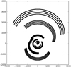 |
Fig. 1 Plot of the uv coverage of a small subset of an observation. Parallel tracks are for the same baseline, but different for frequencies. |
 |
Fig. 2 Panel a: track in uv domain fora single baseline and multiple channels. The boxes indicate the position of the subgrids. The bold box corresponds to the bold samples. Panel b: single subgrid (box) encompassing all affected pixels in the uv grid. The support of the convolution function is indicated by the circles around the samples. |
3.3 Gridding equation in the image domain
A shift from (u0p, v0p) to the origin can be written as a convolution by the Dirac delta function  . Partitioning the gridding Eq. (12) into groups and factoring out the shift for the central pixel leads to
 (22)
(22)
The shifts in the inner and outer summation cancel each other, leaving only the shift in the original Eq. (12).
Now define subgrid  as the result of the inner summation in the equation above
 (23)
(23)
The uv grid  is then a summation of shifted subgrids
  :
:
 (24)
(24)
Now we define the subgrid image  as the inverse Fourier transform of
  . The subgrids
  can then be computed by first computing
  and then transforming it to the uv domain. The equation for the subgrid image,
  , can be found from its definition:
 (25)
(25)
This equation is very similar to the direct imaging Eq. (11). An important difference is the shift towards the origin making the remaining terms  and
and  much smaller thanthe uk and vk in the original equation. That means that the discrete version of this equation can be sampled by far fewer pixels. In fact, image
  is critically sampled when the number of pixels equals the size of the enclosing box in the uv domain. A denser sampling is not needed since the Fourier transform of a denser sampled image will result in near zero values in the region outside the enclosing box. The sampled versions of the subgrid and subgrid image are denoted by
 ![Mathematical equation: $\widehat{V}_p[i,j]$](/articles/aa/full_html/2018/08/aa32858-18/aa32858-18-eq52.png) and
and ![Mathematical equation: $\widehat{I}_p[i,j]$](/articles/aa/full_html/2018/08/aa32858-18/aa32858-18-eq53.png) , respectively.
, respectively.
Because  can be sampled on a grid with far fewer samples than the original image, it is not particularly expensive to compute
  by first computing a direct image using Eq. (25) and then applying the FFT. The subgrid
  can then be added to the master grid. The final image
  is then the inverse Fourier transform of
  divided by the root mean square (rms) window
  .
.
Discretization of the equations above leads to Algorithms 1 and 2 for gridding and degridding, respectively.
Image domain gridding
Image domain degridding
3.4 Variations
The term forthe “convolution function” ![Mathematical equation: $c_{\textrm{pk}} \left[i,j\right]$](/articles/aa/full_html/2018/08/aa32858-18/aa32858-18-eq60.png) is kept very generic here by giving it an index k, allowing a different value for each sample. Often the gain term, included in cpk, can be assumed constant over many data points. The partitioning of the data can be done such that only a single cp for each block is needed. The multiplication by ck can then be pulled outside the loop over the visibilities, reducing the number of operations in the inner loop.
is kept very generic here by giving it an index k, allowing a different value for each sample. Often the gain term, included in cpk, can be assumed constant over many data points. The partitioning of the data can be done such that only a single cp for each block is needed. The multiplication by ck can then be pulled outside the loop over the visibilities, reducing the number of operations in the inner loop.
In the polarized case each antenna consists of two components, each measuring a different polarization, the visibilities are 2 × 2 matrices and the gain g is described by a 2 × 2 Jones matrix. For this case the algorithm is not fundamentally different. Scalar multiplications are substituted by matrix multiplications, effectively adding an extra loop over the different polarizations of the data, and an extra loop over the differently polarized images.
4 Analysis
In the previous section, the image domain gridding algorithm is derived rather intuitively without considering the effects of sampling and truncation, except for the presence of a still-unspecified anti-aliasing window c[i, j]. In this section, the output of the algorithm is analyzed in more detail. The relevant metric here is the difference between the result of direct imaging/evaluation and gridding/degridding, respectively. This difference, or gridding error, is due solely to the side lobes of the anti-aliasing window. These side lobes are caused by the limited support of the gridding kernel. An explicit expression for the error will be derived in terms of the anti-aliasing window. Minimization of this expression leads directly to the optimal window, and corresponding error. This completes the analysis of accuracy of image domain gridding, except for the effect of limited numerical precision, which was found in practice not to be a limiting factor.
For comparison, we summarize the results on the optimal anti-aliasing window for classical gridding known in the literature. For both classical and image domain gridding the error can be made arbitrarily small by selecting a sufficiently large kernel. It is shown below that both methods reach comparable performance for equal kernel sizes. Conversely, to reach a given level of performance both methods need kernels of about the same size.
4.1 Optimal windows for classical gridding
We restrict the derivation of the optimal window in this section to a 1D window f(x). The spatial coordinate is now x, replacing the l, m pair in the 2D case, and normalized such that the region to be imaged, or the main lobe, is given by − 1∕2 ≤ x < 1∕2. The 2D windows used later on are a simple product of two one-dimensional (1D) windows, c(l, m) = f(l∕S)f(m∕S), and it is assumed that optimality is mostly preserved. Brouw (1975) uses as criterion for the optimal window that it maximizes the energy in the main lobe relative to the total energy:
 (26)
(26)
under the constraint that its support in the uv domain is not larger than a given kernel size β. This minimization problem was already known in other contexts. In Slepian & Pollak (1961) and Landau & Pollak (1961), it is shown that this problem can be written as an eigenvalue problem. The solution is the prolate spheroidal wave function (PSWF). The normalized energy in the side lobes is defined by
 (27)
(27)
For the PSWF, the energy in the side lobes is related to the eigenvalue:
 (28)
(28)
where λ0(α) is the first eigenvalue and α = βπ∕2. The eigenvalue is given by
![Mathematical equation: \begin{equation*} \lambda_0(\alpha) = \frac{2\alpha}{\pi}\left[R_{00}(\alpha,1)\right]^2, \end{equation*}](/articles/aa/full_html/2018/08/aa32858-18/aa32858-18-eq64.png) (29)
(29)
where Rmn(c, η) is the radial prolate spheroidal wave function (Abramowitz & Stegun 1965, Ch. 21).
The second column of Table 1 shows the aliasing error ε for different β. The required kernel size can be found by looking up the smallest kernel that meets the desired level of performance.
Level of aliasing for different gridding methods and kernel sizes.
4.2 Effective convolution function in image domain gridding
In classical gridding, the convolution by a kernel in the uv domain effectively applies a window in the image domain. In image domain gridding, the convolution by a kernel is replaced by a multiplication on a small grid in the image domain by a discrete taper c[i, j]. Effectively, this applies a (continuous) window on the (entire) image domain, like in classical gridding. Again the 2D taper is chosen to be a product of two 1D tapers:
![Mathematical equation: \begin{equation*} c[i,j] = a_i a_j. \end{equation*}](/articles/aa/full_html/2018/08/aa32858-18/aa32858-18-eq65.png) (30)
(30)
The 1D taper is described by the set of coefficients {ak}.
It can be shown that the effective window is a sinc interpolation of the discrete window. The interpolation however is affected by the multiplication by the phase gradient corresponding to the position shift from the subgrid center, Δ u, Δv. For the 1D analysis, we use a single parameter for the position shift, s.
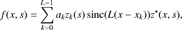 (31)
(31)
where z(x, s) is the phase rotation corresponding to the shift s, and sinc(x) is the normalized sinc function defined by
 (32)
(32)
Phasor z(x, s) is given by
 (33)
(33)
The sample points are given by xk = −1∕2 + k∕L. The phasor at the sample points is given by zk(s) = z(xk, s). Although the gradients cancel each other exactly at the sample points, the effect of the gradient can still be seen in the side lobes. The larger the gradient, the larger the ripples in the sidelobes, as can be seen in Fig. 3. Larger gradients correspond to samples further away from the subgrid center.
The application of the effective window can also be represented by a convolution in the uv domain, whereby thekernel depends on the position of the sample within the subgrid. Figures 4a-c show the convolution kernel for different position shifts. For samples away from the center the convolution kernel is asymmetric. That is because each sample affects all points in the sub-grid, and not just the surrounding points as in classical gridding. Samples away from the center have more neighboring samples on one side than the other. In contrast to classical gridding, the convolution kernel in image domain gridding has side lobes. These side lobes cover the pixels that fall within the sub-grid, but outside the main lobe of the convolution kernel.
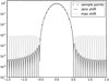 |
Fig. 3 Effective window depending on the position of the sample within the sub-grid. The lowest side lobes are for a sample in the center of the sub-grid. The higher side lobes for samples close to the edge are caused by the phase gradient corresponding to a shift away from the center. |
4.3 Optimal window for image domain gridding
The cost function that is minimized by the optimal window is the mean square of the side lobes of the effectivewindow. Because the effective window depends on the position within the sub-grid, the mean is also taken over all allowed positions. For a convolution kernel with main lobe width β, the shift away from the sub-grid center ∥s∥ cannot be more than (L − β + 1)∕2, because then the main lobe wraps around far enough to touch the first pixel on the other side. This effect can be seen in Fig. 4d. The samples in the center have a low error. The further the sample is from the center, the larger is thepart of the convolution kernel that wraps around, and the larger are the side lobes of the effective window.
The cost function to be minimized is given by
 (34)
(34)
In the Appendix a L × L matrix  is derived such that the error can be written as
 (35)
(35)
where ![Mathematical equation: $\mathbf{a} = \left[\begin{array}{ccc}{a_0 \cdots a_{L-1}}\end{array}\!\!\!\right]$](/articles/aa/full_html/2018/08/aa32858-18/aa32858-18-eq72.png) is a vector containing the window’s coefficients. The minimization problem
is a vector containing the window’s coefficients. The minimization problem
 (36)
(36)
can be solved by a eigenvalue decomposition of 
 (37)
(37)
The smallest eigenvalue λL−1 gives the side lobe level ε for the optimal window aopt = uL−1.
The shape of the convolution kernel is a consequence of computing the cost function as the mean over a range of allowed shifts − (L − β + 1) ≤ s ≤ L − β + 1. The minimization of the cost function leads to a convolution kernel with a main lobe that is approximately β pixels wide, but this width is not enforced by any other means than through the cost function.
Table 1 shows the error level for various combinations of sub-grid size L and width β. For smaller sub-grids the aliasing for image domain gridding is somewhat higher than for classical gridding with the PSWF, but, perhaps surprisingly, for larger sub-grids the aliasing is lower. This is not in contradiction with the PSWF being the convolution function with the lowest aliasing for a given support size. The size of the effective convolution function of image domain gridding is L, the width of the sub-grid, even though the main lobe has only size β. Apparently, the side lobes of the convolution function contribute a little to alias suppression.
In the end, the exact error level is of little importance. One can select a kernel size that meets the desired performance. Table 1 shows that kernel size in image domain gridding will not differ much from the kernel size required in classical gridding. For a given kernel size, there exists a straightforward method to compute the window. In practice, the kernel for classical gridding is often sampled. In that case, the actual error is larger than derived here. Image domain gridding does not need a sampled kernel and the error level derived here is an accurate measure for the level reached in practice.
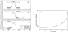 |
Fig. 4 Panels a–c: effective convolution function for samples at different positions within the sub-grid; panel a: sample at the center ofthe sub-grid; panel b: sample at the leftmost position within the sub-grid before the main lobe wraps around; panel c: sample at the rightmost position within the sub-grid before the main lobe wraps around. Panel d: gridding error as a function of position of the sample within the sub-grid. Close to the center of the sub-grid the error changes little with position. The error increases quickly with distance from the center immediately before the maximum distance is reached. |
5 Application to simulated and observed data
In the previous section, it was shown that by proper choice of the tapering window the accuracy of image domain gridding is at least as good as classical gridding. The accuracy at the level of individual samples was measured based on the root mean square value of the side lobes of the effective window. In practice, images are made by integration of very large datasets. In this section we demonstrate the validity of the image domain gridding approach by applying the algorithm in a realistic scenario to both simulated and observed data, and comparing the result to the result obtained using classical gridding.
5.1 Setup
The dataset used is part of a LOFAR observation of the “Toothbrush” galaxy cluster by van Weeren et al. (2016). For the simulations, this dataset was used as a template to generate visibilities with the same metadata as the preprocessed visibilities in the dataset. The pre-imaging processing steps of flagging, calibration and averaging in time and frequency had already been performed. The dataset covers ten LOFAR sub-bands whereby each sub-band is averaged down to 2 channels, resulting in 20 channels covering the frequency range 130–132 MHz. The observation included 55 stations, where the shortest baseline is 1 km, and the longest is 84 km. In time, the data were averaged to intervals of 10 s. The observation lasted 8.5 h, resulting in 3122 timesteps, and, excluding autocorrelations, 4 636 170 rows in total.
The imager used for the simulation is a modified version of WSClean (Offringa et al. 2014). The modifications allow the usage of the implementation of image domain gridding by Veenboer et al. (2017) instead of classical gridding.
5.2 Performance metrics
Obtaining high-quality radio astronomical images requires deconvolution. Deconvolution is an iterative process. Some steps in the deconvolution cycle are approximations. Not all errors thus introduced necessarily limit the final accuracy that can be obtained. In each following iteration, the approximations in the previous iterations can be corrected for. The computation of the residual image however is critical. If the image exactly models the sky then the residual image should be noise only, or zero in the absence of noise. Any deviation from zero sets a hard limit on the attainable dynamic range.
The dynamic range can also be limited by the contribution of sources outside the field of view. Deconvolution will not remove this contribution. The outside sources show up in the image through side lobes of the point spread function (PSF) around the actual source, and as alias inside the image. The aliases are suppressed by the anti-aliasing taper.
The PSF is mainly determined by the uv coverage and the weighting scheme, but the gridding method has some effect too. A well-behaved PSF allows deeper cleaning per major cycle, reducing the number of major cycles.
The considerations above led to the following metrics for evaluation of the image domain gridding algorithm:
level of the side lobes of the PSF;
root mean square level of the residual image of a simulated point source, where the model image and the model to generate the visibilities are an exact match;
the rms level of a dirty image of a simulated source outside the imaged area.
5.3 Simulations
The simulation was set up as follows. An empty image of 2048 × 2048 pixels was generated with cell size of 1 arcsec. A single pixel at position (1000, 1200) in this image was set to 1.0 Jy.
The visibilities for this image were computed using three different methods: (1) direct evaluation of the ME, (2) classical degridding, and (3) image domain degridding. For classical gridding we used the default WSClean settings: a Kaiser–Bessel (KB) window of width 7 and oversampling factor 63. The KB window is easier to compute than the PSWF, but its performance is practically the same. For image domain gridding, a rather large sub-grid size of 48 × 48 pixels was chosen. A smaller sub-grid size could have been used if the channels had been partitioned into groups, but this was not yet implemented.
The image domain gridder ran on a NVIDIA GeForce 840M, a GPU card for laptops. The CPU is a dual core Intel i7 (with hyperthreading) running at 2.60 GHz clockspeed.
The runtime is measured in two ways: (1) at the lowest level, purely the (de)gridding operation and (2) at the highest level, including all overhead. The low-level gridding routines report their runtime and throughput. WSClean reports the time spend in gridding, degridding, and deconvolution. The gridding and degridding times reported by WSClean include the time spent in the large-scale FFTs and reading and writing the data and any other overhead.
The speed reported by the gridding routine was 4.3 M visibilities s−1. For the 20 × 4636170 = 93 M visibilities in the dataset, the gridding time is 22 s. The total gridding time reported by WSClean was 72 s.
The total runtime for classical gridding was 52 s for Stokes I only, and 192 s for all polarizations. The image domain gridder always computes all four polarizations.
Figure 5 shows the PSF. In the main lobe the difference between the two methods is small. The side lobes for the image domain gridder are somewhat (5%) lower than for classical gridder. Although in theory this affects the cleaning depth per major cycle, we do not expect such a small difference to have a noticable impact on the convergence and total runtime of the deconvolution.
A much larger difference can be seen in the residual visibilities in Fig. 6 and the residual image in Fig. 7. The factor-18 lower noise in the residual image means an increase of the dynamic range limit by that factor. This increase will of course only be realized when the gridding errors are the limiting factor.
In Fig. 8 a modest 2% better suppression of an outlier source is shown. This will have little impact on the dynamic range.
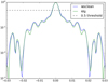 |
Fig. 5 PSF for the classical gridder (blue) and the image domain gridder (green) on a logarithmic scale. The main lobes are practically identical. The first side lobes are a bit less for the image domain gridder. There are some differences in the further (lower) sidelobes as well, but without a consistent pattern. The rms value over the entire image, except the main lobe, is about 5% lower for image domain gridding than for classical gridding. |
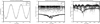 |
Fig. 6 Left panel: real value of visibilities for a point source as predicted by direct evaluation of the ME, and degridding by the classical gridder and image domain gridder. The visibilities are too close together to distinguish in this graph. Middle and right panels: absolute value of the difference between direct evaluation and degridding for a short (1 km) and a long (84 km) baseline. On the short baseline, the image domain gridder rms error of 1.03e-05 Jy is about 242 times lower than the classical gridder rms error of 2.51e-03 Jy. On the long baseline, the image domain gridder rms error of 7.10e-04 Jy is about seven times lower than the classical gridder error of 4.78e-03 Jy. |
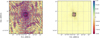 |
Fig. 7 Residual image for the classical gridder in wsclean (left panel) and the image domain gridder (right panel). The color-scale for both images is the same, ranging from –1.0e-05 Jy beam−1 to 1.0e-05 Jybeam−1. The rms value of the area in the box centered on the source is about 19 times lower for image domain gridding (7.6e-06 Jy beam−1) than for classical gridding (1.3e-4 Jy beam−1). The rms value over the entire image is about 17 times lower for image domain gridding (1.1e-06 Jy beam−1) than for classical gridding (2.1e-05 Jy beam−1) |
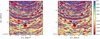 |
Fig. 8 Image of simulated data of a source outside the field of view with classical gridding (left panel) and image domain gridding (right panel). The color-scale for both images is the same, ranging from –1.0e-03 Jy beam−1 to 1.0e-03 Jybeam−1. Position of the source is just outside the image to the north. The aliased position of the source within the image is indicated by an “X”. The image is the convolution of the PSF with the actual source and all its aliases. In the image for the classical gridder (left panel), the PSF around the alias is just visible. In the image for the image domain gridder (right panel), the alias is almost undetectable. The better alias suppressionhas little effect on the overall rms value since this is dominated by the side lobes of the PSF around theactual source. The rms value over the imaged area is 2% lower for image domain gridding (1.35 Jy beam−1) than for classical gridding (1.38e-03 Jy beam−1). |
5.4 Imaging observed data
This imaging job was run on one of the GPU nodes of LOFAR Central Processing cluster. This node has two Intel(R) Xeon(R) E5–2630 v3 CPUs running at 2.40 GHz. Each CPU has eight cores. With hyperthreading, each core can run 2 threads simultaneously. All in all, 32 threads can run in parallel on this node.
The node also has four NVIDIA Tesla K40c GPUs. Each GPU has a compute power of 4.29 Tflops (single precision).
The purpose of this experiment is to measure the run time of an imaging job large enough to make a reasonable extrapolation to a full-size job. This is not a demonstration of the image quality that can be obtained, because that requires a more involved experiment. For example, direction-dependent corrections are applied, but they were filled with identity matrices. Their effect is seen in the runtime, but not in the image quality.
The dataset is again the “toothbrush” dataset used also for the simulations. The settings are chosen to image the full field of LOFAR at the resolution for an observation including all remote stations (but not the international stations). The image computed is 30 000 × 30 000 pixels with 1.2 asec pixel−1.
After imaging 10% was clipped on each side, resulting in a 24 000 × 24 000 pixel image, or 8 deg × 8 deg. The weighting scheme used is Briggs’ weighting, with the robustness parameter set to 0. The cleaning threshold is set to 100 mJy, resulting in four iterations of the major cycle. Each iteration takes about 20 min. Figure 9 shows the resulting image.
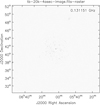 |
Fig. 9 Large image (20 000 × 20 000 pixel) of the toothbrush field. The field of view is 22° × 22°at a resolution of 4 arcsec per pixel. Cleaned down to 100 mJy per beam, taking four major cycles. |
6 Conclusions and future work
The image domain gridding algorithm is designed for the case where the cost of computing the gridding kernels is a significant part of the total cost of gridding. It eliminates the need to compute a (sampled) convolution kernel by directly working in the image domain. This not only eliminates the cost of computing a kernel, but is also more accurate compared to using an (over) sampled kernel.
Although the computational cost of the new algorithm is higher in pure operation count than classical gridding, in practice it performs very well. On some (GPU) architectures it is even faster than classical gridding even when the cost of computing the convolution functions is not included. This is a large step forward, since it is expected that for the square kilometer array (SKA), the cost of computing the convolution kernels will dominate the total cost of gridding.
Both in theory and simulation, it has been shown that image domain gridding is at least as accurate as classical gridding as long as a good taper is used. The optimal taper has been derived.
The originally intended purpose of image domain gridding, fast application of time and direction dependent corrections, has not yet been tested, as the corrections for the tests in this paper have been limited to identity matrices. The next step is to use image domain gridding to apply actual corrections.
Another possible application of image domain gridding is calibration. In calibration, a model is fitted to observed data. This involves the computation of residuals and derivatives. These can be computed efficiently by image domain gridding whereby the free parameters are the A-term. This would allow to fit directly for an A-term in the calibration step, using a full image as a model.
Acknowledgements
This work was supported by the European Union, H2020 program, Astronomy ESFRI and Research Infrastructure Cluster (Grant Agreement No. 653477). The first author would like to thank Sanjay Bhatnagar and others at NRAO, Soccoro, NM, USA, for their hospitality and discussions on the A-projection algorithm in May 2011 that ultimately were the inspiration for the work presented inthis paper. We would also like to thank A.-J. van der Veen for his thorough reading of and comments on a draft version.
Appendix A Derivation of the optimal window
The optimal window is derived by writing out the expression for the mean energy in the side lobes in terms of coefficients ak. This expression contains a double integral: one integral is over the extent of the side lobes, and one over all allowed positions in the sub-grid. The double integral can be expressed in terms of special functions. The expression for the mean energy then reduces to a weighted vector norm, where the entries of the weighting matrix are given in terms of the special functions. The minimization problem can then readily be solved by singular value decomposition.
The square of the effective window given in Eq. (31) is
 (A.1)
(A.1)
This can be written as a matrix product:
 (A.2)
(A.2)
where the elements of matrix Q(x) are given by qi,j = sinc(x − k)sinc(x − l) and the elements of matrix S(s) are given by  . The equation for the error Eq. (34) can now be written as
 (A.3)
(A.3)
where  and
and
 (A.4)
(A.4)
and
 (A.5)
(A.5)
To evaluate the entries of  , the following integral is needed:
![Mathematical equation: \begin{eqnarray*} & \int \frac{\sin^2(\pi x)}{\pi^2(x^2 + kx)}dx = \frac{1}{2\pi^2k}\left( \operatorname{Ci}(2\pi(k+x)) - \log(k+x) \right.\nonumber \\[4pt] & \quad\ \left. -\operatorname{Ci}(2\pi x) + \log(x) \right), \quad \forall k \in \mathbb{Z}, \end{eqnarray*}](/articles/aa/full_html/2018/08/aa32858-18/aa32858-18-eq84.png) (A.6)
(A.6)
where Ci(x) is the cosine integral, a special function defined by
 (A.7)
(A.7)
The entries of matrix  are given by
![Mathematical equation: \begin{eqnarray*} \bar{s}_{kl} & = \frac{1}{L-\ +1}\int_{-(L-\beta+1)/2}^{(L-\beta+1)/2} \textrm{e}^{\frac{j 2\pi (k-l) s}{L}} \textrm{d}s\nonumber \\[2pt] & = \frac{1}{L-\beta+1}\left[ -\frac{jL}{2\pi (k-l)} \textrm{e}^{\frac{j2\pi (k-l) s}{L}} \right]_{-(L-\beta+1)/2}^{(L-\beta+1)/2}\nonumber \\[2pt] & = \frac{L}{\pi (k-l)(L-\beta+1)} \sin(\pi (k-l) (L-\beta+1)/L)\nonumber \\[3pt] & = \operatorname{sinc}((k-l)(L-\beta+1)/N). \end{eqnarray*}](/articles/aa/full_html/2018/08/aa32858-18/aa32858-18-eq87.png) (A.8)
(A.8)
References
- Abramowitz, M. & Stegun, I. A., eds. 1965, Handbook of Mathematical Functions with Formulas, Graphs and Mathematical Tables (New York: Dover Publications, Inc.) [Google Scholar]
- Bhatnagar, S., Cornwell, T. J., Golap, K., & Uson, J. M. 2008, A&A, 487, 419 [NASA ADS] [CrossRef] [EDP Sciences] [Google Scholar]
- Brouw, W. N. 1975, in Methods in Computational Physics. Volume 14 – Radio Astronomy, eds. B. Alder, S. Fernbach, & M. Rotenberg, 14, 131 [NASA ADS] [Google Scholar]
- Cornwell, T. J., & Perley, R. A. 1992, A&A, 261, 353 [NASA ADS] [Google Scholar]
- Cornwell, T., Golap, K., & Bhatnagar, S. 2005, Astronomical Data Analysis Software and Systems XIV, 347, 86 [NASA ADS] [Google Scholar]
- Cornwell, T., Golap, K., & Bhatnagar, S. 2008, IEEE J. Sel. Top. Signal Process., 2, 647 [NASA ADS] [CrossRef] [Google Scholar]
- Cornwell, T. J., Voronkov, M. A., & Humphreys, B. 2012, in Image Reconstruction from Incomplete Data VII, Proc. SPIE, 8500, 85000L [NASA ADS] [CrossRef] [Google Scholar]
- Hamaker, J. P. 2000, A&AS, 143, 515 [NASA ADS] [CrossRef] [EDP Sciences] [Google Scholar]
- Hamaker, J. P., Bregman, J. D., & Sault, R. J. 1996, A&AS, 117, 137 [NASA ADS] [CrossRef] [EDP Sciences] [Google Scholar]
- Humphreys, B., & Cornwell, T. J. 2011, SKA MEMO 132, https://www.skatelescope.org/uploaded/59116_132_Memo_Humphreys.pdf [Google Scholar]
- Johansson, F. et al. 2014, mpmath: A Python Library for Arbitrary-Precision Floating-point Arithmetic (Version 0.19), http://mpmath.org/ [Google Scholar]
- Landau, H. J., & Pollak, H. O. 1961, Bell Syst. Tech. J., 40, 65 [CrossRef] [Google Scholar]
- Offringa, A. R., McKinley, B., Hurley-Walker, N., et al. 2014, MNRAS, 444, 606 [NASA ADS] [CrossRef] [Google Scholar]
- Slepian, D., & Pollak, H. O. 1961, Bell Syst. Tech. J., 40, 43 [CrossRef] [Google Scholar]
- Smirnov, O. M. 2011, A&A, 527, A106 [NASA ADS] [CrossRef] [EDP Sciences] [Google Scholar]
- Tasse, C., van der Tol, S., van Zwieten, J., van Diepen, G., & Bhatnagar, S. 2013, A&A, 553, A105 [NASA ADS] [CrossRef] [EDP Sciences] [Google Scholar]
- Tasse, C., Hugo, B., Mirmont, M., et al. 2018, A&A, 611, A87 [Google Scholar]
- Taylor, G. B., Carilli, C. L., & Perley, R. A. 1999, Synthesis Imaging in Radio Astronomy II, ASP Conf. Ser., 180 [Google Scholar]
- van der Tol, S. 2017, Fast Method for Gridding and Degridding of Fourier Component Measurements for Image Reconstruction, http://worldwide.espacenet.com/textdoc?DB=EPODOC&IDX=NL1041834 [Google Scholar]
- van Weeren, R. J., Brunetti, G., Brüggen, M., et al. 2016, ApJ, 818, 204 [NASA ADS] [CrossRef] [Google Scholar]
- Veenboer, B. 2017, astron-idg, https://gitlab.com/astron-idg [Google Scholar]
- Veenboer, B., Petschow, M., & Romein, J. 2017, IEEE International Parallel and Distributed Processing Symposium (IPDPS), 445 [Google Scholar]
- Young, A., Wijnholds, S. J., Carozzi, T. D., et al. 2015, A&A, 577, A56 [NASA ADS] [CrossRef] [EDP Sciences] [Google Scholar]
See footnote on p. 128 of Taylor et al. (1999) on why DFT is a misnomer for this equation.
All Tables
All Figures
|
Fig. 1 Plot of the uv coverage of a small subset of an observation. Parallel tracks are for the same baseline, but different for frequencies. |
| In the text | |
|
Fig. 2 Panel a: track in uv domain fora single baseline and multiple channels. The boxes indicate the position of the subgrids. The bold box corresponds to the bold samples. Panel b: single subgrid (box) encompassing all affected pixels in the uv grid. The support of the convolution function is indicated by the circles around the samples. |
| In the text | |
|
Fig. 3 Effective window depending on the position of the sample within the sub-grid. The lowest side lobes are for a sample in the center of the sub-grid. The higher side lobes for samples close to the edge are caused by the phase gradient corresponding to a shift away from the center. |
| In the text | |
|
Fig. 4 Panels a–c: effective convolution function for samples at different positions within the sub-grid; panel a: sample at the center ofthe sub-grid; panel b: sample at the leftmost position within the sub-grid before the main lobe wraps around; panel c: sample at the rightmost position within the sub-grid before the main lobe wraps around. Panel d: gridding error as a function of position of the sample within the sub-grid. Close to the center of the sub-grid the error changes little with position. The error increases quickly with distance from the center immediately before the maximum distance is reached. |
| In the text | |
|
Fig. 5 PSF for the classical gridder (blue) and the image domain gridder (green) on a logarithmic scale. The main lobes are practically identical. The first side lobes are a bit less for the image domain gridder. There are some differences in the further (lower) sidelobes as well, but without a consistent pattern. The rms value over the entire image, except the main lobe, is about 5% lower for image domain gridding than for classical gridding. |
| In the text | |
|
Fig. 6 Left panel: real value of visibilities for a point source as predicted by direct evaluation of the ME, and degridding by the classical gridder and image domain gridder. The visibilities are too close together to distinguish in this graph. Middle and right panels: absolute value of the difference between direct evaluation and degridding for a short (1 km) and a long (84 km) baseline. On the short baseline, the image domain gridder rms error of 1.03e-05 Jy is about 242 times lower than the classical gridder rms error of 2.51e-03 Jy. On the long baseline, the image domain gridder rms error of 7.10e-04 Jy is about seven times lower than the classical gridder error of 4.78e-03 Jy. |
| In the text | |
|
Fig. 7 Residual image for the classical gridder in wsclean (left panel) and the image domain gridder (right panel). The color-scale for both images is the same, ranging from –1.0e-05 Jy beam−1 to 1.0e-05 Jybeam−1. The rms value of the area in the box centered on the source is about 19 times lower for image domain gridding (7.6e-06 Jy beam−1) than for classical gridding (1.3e-4 Jy beam−1). The rms value over the entire image is about 17 times lower for image domain gridding (1.1e-06 Jy beam−1) than for classical gridding (2.1e-05 Jy beam−1) |
| In the text | |
|
Fig. 8 Image of simulated data of a source outside the field of view with classical gridding (left panel) and image domain gridding (right panel). The color-scale for both images is the same, ranging from –1.0e-03 Jy beam−1 to 1.0e-03 Jybeam−1. Position of the source is just outside the image to the north. The aliased position of the source within the image is indicated by an “X”. The image is the convolution of the PSF with the actual source and all its aliases. In the image for the classical gridder (left panel), the PSF around the alias is just visible. In the image for the image domain gridder (right panel), the alias is almost undetectable. The better alias suppressionhas little effect on the overall rms value since this is dominated by the side lobes of the PSF around theactual source. The rms value over the imaged area is 2% lower for image domain gridding (1.35 Jy beam−1) than for classical gridding (1.38e-03 Jy beam−1). |
| In the text | |
|
Fig. 9 Large image (20 000 × 20 000 pixel) of the toothbrush field. The field of view is 22° × 22°at a resolution of 4 arcsec per pixel. Cleaned down to 100 mJy per beam, taking four major cycles. |
| In the text | |
Current usage metrics show cumulative count of Article Views (full-text article views including HTML views, PDF and ePub downloads, according to the available data) and Abstracts Views on Vision4Press platform.
Data correspond to usage on the plateform after 2015. The current usage metrics is available 48-96 hours after online publication and is updated daily on week days.
Initial download of the metrics may take a while.