| Issue |
A&A
Volume 616, August 2018
|
|
|---|---|---|
| Article Number | A75 | |
| Number of page(s) | 7 | |
| Section | Stellar structure and evolution | |
| DOI | https://doi.org/10.1051/0004-6361/201832810 | |
| Published online | 21 August 2018 | |
The triple system HD 150136: From periastron passage to actual masses ★,★★
1
Instituut voor Sterrenkunde, KU Leuven,
Celestijnlaan 200D, Bus 2401,
3001
Leuven,
Belgium
e-mail: laurent.mahy@kuleuven.be
2
Space Sciences, Technologies, and Astrophysics Research (STAR) Institute, Université de Liège, Quartier Agora,
Bât B5c, Allée du 6 août, 19c,
4000
Liège,
Belgium
3
Unidad de Astronomía, Facultad de Ciencias Básicas, Universidad de Antofagasta,
Antofagasta,
Chile
4
Astronomical Institute ASCR,
Fricova 298,
251 65
Ondrejov,
Czech Republic
5
Visitor Scientist at Gemini Observatory, Northern Operations Center,
670 North A’ohoku Place,
Hilo,
HI 96720,
USA
6
Institute of Astronomy, University of Geneva,
51 chemin des Maillettes,
1290
Versoix,
Switzerland
7
UJF-Grenoble 1/CNRS-INSU, Institut de Planétologie et d’Astrophysique de Grenoble (IPAG),
UMR 5274,
Grenoble,
France
8
Anton Pannekoek Institute for Astronomy, University of Amsterdam,
1090
GE Amsterdam,
The Netherlands
Received:
12
February
2018
Accepted:
30
April
2018
Context. The triple system HD 150136 is composed of an O3 V((f*))–O3.5 V((f+)) primary, of an O5.5–6 V((f)) secondary, and of a more distant O6.5–7 V((f)) tertiary. The latter component went through periastron in 2015–2016, an event that will not occur again within the next eight years.
Aims. We aim to analyse the tertiary periastron passage to determine the orbital properties of the outer system, to constrain its inclination and its eccentricity, and to determine the actual masses of the three components of the system.
Methods. We conducted an intensive spectroscopic monitoring of the periastron passage of the tertiary component and combined the outcoming data with new interferometric measurements. This allows us to derive the orbital solution of the outer orbit in three-dimensional space. We also obtained the light curve of the system to further constrain the inclination of the inner binary.
Results. We determine an orbital period of 8.61 ± 0.02 years, an eccentricity of 0.682 ± 0.002, and an inclination of 106.18 ± 0.14° for the outer orbit. The actual masses of the inner system and of the tertiary object are 72.32−8.49+8.45 M⊙ and 15.54−4.97+4.96 M⊙, respectively. From the mass of the inner system and accounting for the known mass ratio between the primary and the secondary, we determine actual masses of 42.81 M⊙ and 29.51 M⊙ for the primary and the secondary components, respectively. We infer, from the different mass ratios and the inclination of the outer orbit, an inclination of 62.4° for the inner system. This value is confirmed by photometry. Grazing eclipses and ellipsoidal variations are detected in the light curve of HD 150136. We also compute the distance of the system to 1.096 ± 0.274 kpc.
Conclusions. By combining spectroscopy, interferometry, and photometry, HD 150136 offers us a unique chance to compare theory and observations. The masses estimated through our analysis are smaller than those constrained by evolutionary models. The formation of this triple system suggests similar ages for the three components within the errorbars. Finally, we show that Lidov–Kozai cycles have no effect on the evolution of the inner binary, which suggests that the latter will experience mass transfer leading to a merger of the two stars.
Key words: stars: early-type / binaries: spectroscopic / stars: fundamental parameters / stars: individual: HD150136
Based on observations collected at the European Southern Observatory (Paranal and La Silla, Chile).
The journal of observations and the radial velocity data are only available at the CDS via anonymous ftp to cdsarc.u-strasbg.fr (130.79.128.5) or via http://cdsarc.u-strasbg.fr/viz-bin/qcat?J/A+A/616/A75
© ESO 2018
1 Introduction
Massive stars are key objects in the galaxies. They influence both the chemical and the mechanical evolution of their surroundings through the creation of bubbles and of induced or inhibited star formation. They are also the main sources of ultraviolet and ionizing radiations. Despite their importance, actual details of massive star formation and evolution are still to be understood. Most of their fundamental parameters are poorly constrained, especially their masses. In this context, investigating the binary system population is the best way to derive these masses. The relatively small number of extremely massive galactic stars implies that any system whose orbital parameters are accurately determined provides important new constraints to stellar evolution. Binarity, however, affects the way that stars evolve, making their evolution more complex than that of single stars. This is especially relevant for massive stars, given their high fraction of multiple systems (Duchêne & Kraus 2013; Sana et al. 2012, 2014). The situation is even more complex with gravitationally-bound hierarchical systems since the evolution of the stars in those systems can be ruled by the Lidov–Kozai cycles (Kozai 1962; Lidov 1962). The latter can modulate the eccentricity of the inner binary triggering modulations in their interactions (Toonen et al. 2016). In this context, HD 150136 is perfectly suited to better constrain this phenomenon.
This system is one of the two brightest stars hosted in the center of the young open cluster NGC 6193 in the Ara OB1 association, for which the distance was first estimated by Herbst & Havlen (1977) to be 1.32 kpc. This object is a triple hierarchical system formed of an inner binary with an O3 V((f*))–O3.5 V((f+)) primary andan O5.5–6 V((f)) secondary1, orbiting around each other with a period of 2.67455 days, and of an O6.5–7 V((f)) physically bound tertiary component located on a much longer orbit (Mahy et al. 2012). This object is the nearest system harbouring an O3 star. It thus constitutes a target of choice for investigating the fundamental parameters of such a star.
HD 150136 is one of the X-ray-brightest massive stars known (log LX = 33.39 (cgs), log (LX∕Lbol) = −6.4; Skinner et al. 2005), most likely as the result of a radiative colliding-wind interaction. Its X-ray light curve, however, presents variations whose origin remains unclear. The star was also reported as a non-thermal radio emitter (Benaglia et al. 2006; De Becker 2007). This suggests that the system harbours a relativistic population of electrons, probably accelerated through shocks in colliding-wind regions. Mahy et al. (2012) showed that a non-thermal radio emission originating in the inner system would hardly escape. The presence of the third object is thus required in order to displace the emitting region in the outer system.
Following the study of Mahy et al. (2012), the third component is expected to be sufficiently far from the inner system to be observable with long baseline interferometric facilities. The first detections of the outer pair were reported by Sana et al. (2013) from the Precision Integrated-Optics Near-infrared Imaging ExpeRiment (PIONIER) and by Sanchez-Bermudez et al. (2013) from the Astrometrical Multi BEam combineR (AMBER). Sana et al. (2013) combined the preliminary interferometric observations with high-resolution spectroscopic data to derive a first orbital solution of the outer companion in the three-dimensional space. These authors reported a period of 3008 days, and an eccentricity of 0.73 for the outer orbit. Meanwhile, interferometric and spectroscopic observations continue to be obtained to constrain the full orbit. With the analysis of these data, we realized that the expected periastron passage was not yet observed and that the values provided by Sana et al. (2013) needed to be revised. The parameters of the outer orbit were updated through the analysis of the interferometric data by Le Bouquin et al. (2017). The latter changed the values of the period and of the eccentricity to 3067 days and 0.68, and inferred actual masses of 87 M⊙ for the inner system and of 27 M⊙ for the third component. However their lack of spectroscopic observations close to the periastron passage prevented them from strictly constraining the semi-amplitude of the outer orbit and therefore the minimum masses.
This emphasizes the uncertainties linked to the determination of the dynamical masses of the three components. It indeed depends on the maxima of amplitudes of the radial velocity (RV) curves for the outer orbit. In this context, we have undertaken a spectroscopic monitoring covering both sides of the periastron passage of the tertiary component.
The present paper provides the analysis of the new spectroscopic data coupled with new interferometric and with unprecedented photometric observations of HD 150136. The paper is organized as follows. In Sect. 2, we present the observational campaign and the different instruments used. Section 3 is devoted to the determination of the radial velocities of the three components. Section 4 presents the global orbital solution for the inner and the outer systems by combining spectroscopy and interferometry. The light curve of the system is studied in Sect. 5. Section 6 discusses the evolutionary statuses of the different components and, finally, we give our conclusions in Sect. 7.
2 Observations and data reduction
2.1 Spectroscopic observations
We collected and retrieved 177 optical spectra of HD 150136 obtained with the Fibre-fed Extended Range Optical Spectrograph (FEROS) mounted successively on the ESO 1.52 m (for observations before 2002) and on the MPG/ESO 2.2 m (for observations after 2002) telescopes at La Silla observatory (Chile). These data were partially presented and analysed in Mahy et al. (2012) and in Sana et al. (2013) but spectra that were newly acquired around the periastron passage of the third component are introduced in the present paper. The monitoring of HD 150136 on FEROS started in 1999, and went on every year until 2016, with breaks in 2007 and in 2010. FEROS provides a resolving power of R = 48 000 and covers the entire optical range from 3800 to 9200 Å. The data were reduced following the procedure described in Mahy et al. (2012).
We also obtained Director’s Discretionary Time (DDT) with the UV-Visual Echelle Spectrograph (UVES; PI: Mahy 297.D-5007, PI: Gosset 295.D-5025, and PI: Gosset 294.D-5041) mounted on the ESO-VLT to acquire eight additional spectra, which we have completed with two additional spectra provided by the EDIBLES team (see Cox et al. 2017; PI: Cox; Large Programme: 194.C-0833(C)) taken in June and July 2015. These data have a resolving power of R = 80 000. The eight DDT time spectra were acquired with the DIC 2 437+760 setup whilst the spectra taken in June and in July were obtained with the DIC 1 346+564 and the DIC 1 437+860 setups, respectively. The data reduction was performed with the standard reduction pipeline.
Finally, we took three spectra of HD 150136 with the CORALIE spectrograph mounted on the Swiss 1.2 m Leonhard Euler telescope at La Silla. CORALIE is an improved version of the ELODIE spectrograph (Baranne et al. 1996) covering the spectral range between 3850 and 6890 Å. Its resolving power is R = 55 000. The data were reduced with the CORALIE pipeline.
The entire journal of observations is available at the CDS. The heliocentric Julian date (HJD) is the time taken at mid-exposure and is given in the format HJD–2450000.
2.2 Photometric observations
The photometric observations of HD 150136 were carried out between April and August 2017 at Siding Spring Observatory with the 0.43-m f/6.8 telescope (T17) of the iTelescope network2. The camera was equipped with a 1K*1K FLI ProLine E2V CCD47-10-1-109 CCD giving a 15.5′ field at a resolution of 0.92″ pixel−1. A narrow-band O III filter was used in order to avoid saturation of the target star. The observations were made in sequences lasting about 20 minutes of short exposures. The reductions were done with the IRAF daophot packages. The nearby HD 150135 was used as a comparison. It is the only star in the field with a suitable brightness and it proved to be sufficiently stable. An aperture of 3.7 arcsec was used and a small empirical seeing correction was applied because of the nearness of the stars. The best data of each sequence were averaged in order to build the final data set.
2.3 Interferometric observations
In complement to the spectroscopic and photometric data, we also used the astrometric observations compiled by Le Bouquin et al. (2017) to better constrain the orbital parameters of the outer orbit. Two additional points were obtained in May and August 2017 (PI: Sana, 596.D-0495(J)) with the PIONIER combiner (Le Bouquin et al. 2011). We refer to Le Bouquin et al. (2017) for a description of the data reduction procedure.
3 Radial velocity measurements
In order to attain a good accuracy on the radial velocity (RV) measurements, we proceed in different steps to measure them for the three components. In the first step, we fit the line profiles with Gaussian profiles. Given the spectral classification of O3 V((f*))–O3.5 V((f+)) attributed to the primary component, its spectrum presents lines of N V 4604–19 that only this component exhibits. We also focus on the N IV 4058, He II 4542, O III 5592, and He I 5876 lines. The lines formed by elements in higher ionization stages are expected to be created closer to the stellar photospheres, which infers a better estimation of the amplitudes of the RVs. These sets of lines, however, have their disadvantages:
-
the N IV 4058 line is present in emission in the primary spectrum. This line shows an asymmetry that can be due to the wind-wind interaction zone between the primary and the secondary (see Mahy et al. 2012) or to tidal interactions between these two components. Furthermore, this line is contaminated by the C III 4070 line, especially at the maximum of separation, which can make the assessment of asymmetry uncertain;
-
the spectral widths of the He II 4542 lines are different for the three components, given their spectral classifications. Therefore, the primary’s line is the most prominent feature, in comparison with that of the secondary or the tertiary components, making the latter barely detectable outside epochs close to the maxima of separation;
-
the O III 5592 line is not included in the UVES setting, which prevents us from obtaining the related RVs close to the periastron passage;
-
the He I 5876 line is formed further away from the photosphere and can give larger errors on the actual RVs of the components.
To determine the RVs for the three components, we used the rest wavelengths provided by Conti et al. (1977) and Underhill (1995) for wavelengths shorter and longer than 5000 Å, respectively.
In the second step, we disentangled the spectra and refined by cross-correlation the RVs of each component. This method was already described in Mahy et al. (2012), and we refer to this paper for any additional details. This method allows us to obtain RVs, constituting average values on all the line profiles.
We compare the different sets of RVs in Fig. A.1 and we conclude to a global agreement. In the following, we use the set of RVs obtained by cross-correlation, given that they represent average values on several main spectral lines. The RVs are given with the journal of observations that is available at the CDS.
We apply the Heck–Manfroid–Mersch method (Heck et al. 1985), revised by Gosset et al. (2001), on the difference between the RVs of the primary and the secondary to determine the orbital period of the inner (primary/secondary) system and on the RVs of the tertiary component for the orbital period of the outer (primary + secondary/tertiary) system. For the inner system, an outstanding peak at 0.373895 d−1, corresponding to a period of 2.674548 ± 0.000007 days is detected. This value confirms that obtained by Mahy et al. (2012). For the outer system, the periodogram provides an outstanding peak at 0.000318 d−1, corresponding to a period of 3144.7 days, which is slightly larger than the period of 3067 days provided by Le Bouquin et al. (2017).
4 Orbital parameters for the global system
We combine the RV measurements of the three components obtained through spectroscopy with the interferometric datapoints to perform a global fit of the inner and outer orbits. The orbital parameters of the inner system confirm those given by Mahy et al. (2012) and Sana et al. (2013). Figure 1 shows the RV curves of the inner system corrected for the presence of the tertiary.
With the two new interferometric datapoints, the outer orbit is now well constrained, and confirms the values provided by Le Bouquin et al. (2017). The global fit depends on 14 parameters because we keep fixed the eccentricity and the argument of the periastron for the inner system. Besides the orbital parameters, the combination of the astrometric data with the spectroscopic ones from the intensive monitoring during the periastron passage of the tertiary component allows us to obtain more accurate minimum masses than those reported in Sana et al. (2013) and in Le Bouquin et al. (2017). The RV curves computed from the systemic velocities of the inner system at different epochs and from the RVs of the tertiary are shown in the left panel of Fig. 2 whilst the best fit of the relative motion on the sky plane of the tertiary around the inner system is displayed in the right panel of Fig. 2. The global orbital parameters for the inner and the outer systems are listed in Table 1.
By combining the SB3 radial velocity amplitudes with the size and inclination of the relative orbital motion on the sky, it is possible to determine the individual masses of each component and the distance to the system. We use the same approach as that given by Le Bouquin et al. (2017) to estimate the distance and the individual masses of the inner system and the tertiary component (see their Eq. (1)–(3)).
We estimate the total mass of the system to 87.86± 13.71M⊙, given dynamical masses for the inner system of  M⊙ and of
  M⊙ for the third object. From the minimum masses of the primary and secondary components derived from spectroscopy and the dynamical mass of the inner system computed from interferometry, we infer for the inner system an inclination of 62.4°, and provide dynamical masses of 42.81 M⊙ for the primary and of 29.51 M⊙ for the secondary. The inclination is slightly larger than that of 49° estimated inMahy et al. (2012) and in Sana et al. (2013). This yields masses lower than those from the standard values provided by Martins et al. (2005) for stars with these spectral classifications.
To estimate the distance of HD 150136, we compare the two values of the semi-major axis provided by spectroscopy and by interferometry. The distance of HD 150136 is left as a free parameter in our global fitting process. The idea is to compare the values of the semi-major axis provided by spectroscopy and by interferometry by constraining the distance of the system to avoid any correlation between the two values of this parameter. We estimate that HD 150136 is at a distance of 1.096± 0.274 kpc. This value validates the distance of 1.15 kpc for NGC 6193 provided by Kharchenko et al. (2005) even though it does not allow us to reject the distance of 1.32 kpc reported by Herbst & Havlen (1977), which remains within 1σ. If we convert our distance into a parallax value, we obtain  mas. This parallax is then compared tothe recent parallax ϖ = 0.944 ± 0.120 mas provided by Gaia Data Release 2 (Gaia Collaboration 2016, 2018) for HD 150136, showing a very good agreement between both values.
While the inner system is orbiting in the framework of the outer system, its distance to the observer changes with the outer system periodicity. To this distance change, a time-delay effect is associated. The semi-amplitude of this time delay is rather small (< 0.02 days). We correct the observation times of the spectra for the time delay and we re-analyse the inner system data. We recover the same value for parameters indicating the robustness of our solution.
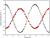 |
Fig. 1 RV curves of the inner system corrected for the presence of the tertiary component. Red dots give the RVs of the primary whilst the black ones indicate the secondary component. |
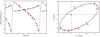 |
Fig. 2 Left panel: RV curves of the outer system. Black dots represent the systemic velocities of the inner (P+S) system whilst the red ones represent the tertiary component. Right panel: relative astrometric orbit of the tertiary component in the outer system; the inner system is considered as fixed at (0,0). The periastron of the tertiary is represented by an open pentagon symbol. The observations are indicated in red and are accompanied with their error ellipses. |
Orbital solution of the inner and outer systems.
5 Photometry
We model the light curve of the inner system by using PHysics Of Eclipsing BinariEs (PHOEBE, v0.31a; Prša & Zwitter 2005) software. The orbital period of the outer orbit being too long, we are not able to see any variations from the tertiary in our light curve. We therefore focus on the parameters of the inner system. We thus keep fixed the parameters of the inner orbit determined through the spectroscopic analysis. PHOEBE allows one to model the light curve and the RV curves of the object at the same time. This software is based on Wilson and Devinney’s code (Wilson & Devinney 1971) and uses Nelder and Mead’s Simplex fitting method to adjust all the input parameters to find the best fit to the light curve. We take into account the effective temperatures of the inner components determined by Mahy et al. (2012), meaning 46 500 and 40 000 K for the primary and the secondary, respectively (see Table 2). We also add a third light for the modelling with a value of 0.156 as estimated from Mahy et al. (2012).
The light curve clearly displays ellipsoidal variations and seemingly grazing eclipses. We confirm the inclination of 62.4° but given the errors on the photometric data, we cannot be more accurate on these values. This result validates our mass estimations for the two components in the inner system, as described in Sect. 4. Figure 3 displays the fit of the light curve obtained by PHOEBE with an inclination of 62.4°. The dispersion around the theoretical light curve seems to be phase dependent (compare both sides of phase 0.25). Additional photometric data are necessary to confirm the last remark as well as the existence and shape of the eclipses.
Top: Observed stellar parameters of the three components; bottom: Stellar parameters derived by BONNSAI.
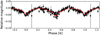 |
Fig. 3 Light curve of HD 150136 (black dots) and the PHOEBE best fit (red). The magnitude outside the eclipses has been set to 0 and lower luminosities correspond to negative values. |
6 Evolutionary status
From the individual parameters determined from photometry, we compute the luminosities of the three components. Based on the determination of the effective temperatures made by Mahy et al. (2012), we compute a luminosity of  for the primary and
 for the secondary. We also use the new distance that we have determined and the brightness factors between the different components given by Mahy et al. (2012) to derive from a different method the luminosities of the three components. We obtain
  , 5.16, and 4.86 for the primary, secondary and tertiary components, respectively, which agrees well with the other above-mentioned values we determined.
These new estimations infer new positions for the three objects in the Hertzsprung–Russell diagram (Fig. 4) compared to those given in Mahy et al. (2012). These new parameters are used as input for BONNSAI3 (Schneider et al. 2014), a publicly available tool, which allows one to derive stellar parameters (e.g., mass, radius, age) from the comparison of a set of observational parameters (e.g., effective temperature, surface gravity, rotational velocity) with the evolutionary tracks of Brott et al. (2011). We use as input the effective temperatures, gravities, luminosities, and projected rotational velocities of the three components. The Bayesian approach provides initial masses of  ,
,  , and
, and  M⊙, for the primary, secondary, and tertiary components, respectively, whilst the actual masses are estimated by BONNSAI to
  ,
,  , and
, and  M⊙, respectively.Compared to the errors on the masses and to the age of the components, the amount of mass lost by the three components during their present lifetime is not yet significant. Whilst the radii and the rotational velocities of the components agree with the observational measurements, the masses are larger than what we found. A general agreement gives an age between 0 and 2 Myrs for the global system. From their radii and their rotational velocities, the two stars of the inner system are in co-rotation with their orbit.
To predict the evolution of HD 150136, we have used the triple-star evolution code TRES (Toonen et al. 2016). We find that the outer star does not affect the evolution of the inner two stars. As the outer period is three orders of magnitude longer than that of the compact inner orbit, the outer and inner orbits are practically kinematically discoupled.
A notorious manifestation of the three-body dynamics are the Lidov–Kozai cycles. During these cycles, the mutual inclination and eccentricity of the inner binary vary periodically. The timescale of these cycles in HD 150136 is about 57 kyrs (based on Kinoshita & Nakai 1999). A higher order level of interaction (i.e. the octupole level) is not strongly relevant for HD 150136 as estimated by the octupole parameter epsilon ϵ = 0.0019 < ϵcritical ≈ 0.01 (see e.g. Naoz et al. 2011).
Regarding the Lidov–Kozai timescale in HD 150136, it is short compared to the stellar lifetimes (>several Myrs), which in principle allows the inner binary to undergo many Lidov–Kozai cycles in its lifetime. However, the cycles are repressed due to strong tidal effects in the inner binary. For this reason, the orbit of the inner binary does not reach significant eccentricities, not even for mutual inclinations of 90 degrees at which the amplitude of the eccentricity cycles is maximized. The evolution of the inner binary is similar to that of an isolated binary.
After a few Myrs (going from 2.6 to 5.5 Myrs, depending on the binary population synthesis code that we use), when both stars will still be on the main sequence, the inner binary will experience mass transfer, leading to a merger of the two stars. According to our simulations, a single main-sequence-like star of ~ 65M⊙ will be created, orbited by the previous tertiary star (see e.g. Glebbeek et al. 2013, for simulations about high-mass stellar mergers).
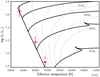 |
Fig. 4 Positions in the Hertzsprung–Russell diagram of the three components of HD 150136. Tracks are from Brott et al. (2011) computed with an initial rotational velocity of about 300 km s−1. |
7 Conclusion
In the present analysis, we have described the observations obtained in spectroscopy during the last periastron passage of the third object composing HD 150136. We have combined them with data from older campaigns and with the astrometric observations either new or previously reported by Le Bouquin et al. (2017), to determine the three-dimensional orbit for the outer system.
In addition to the inclination of the inner and the outer orbits, this study allowed us to constrain with accuracy the dynamical masses of the three objects to  ,
,  , and
, and  M⊙ for the O3, O5.5, and O6 components, respectively. This constitutes the first estimation of the actual mass of a galactic O3 star on the main sequence.
Acknowledgements
We are very grateful to our anonymous referee for his or her remarks and comments with the goal of improving our manuscript. This research was supported by the Fonds National de la Recherche Scientifique (F.R.S.-F.N.R.S.), by the PRODEX XMM contract (Belspo), and through the ARC grant for Concerted Research Actions, financed by the French Community of Belgium (Wallonia-Brussels Federation). We kindly thank Nick Cox and the EDIBLES team for providing advance access to their UVES data for extracting the stellar RV values. AH is supported by the grant 14-02385S from GA ČR. Some of the observations obtained with the MPG 2.2 m telescope were supported by the Ministry of Education, Youth and Sports project– LG14013 (Tycho Brahe: Supporting Ground-based Astronomical Observations). We would like to thank the observers S. Vennes and L. Zychova for obtaining the data. Computational resources were supplied by the Ministry of Education, Youth and Sports of the Czech Republic under the Projects CESNET (Project No. LM2015042) and CERIT-Scientific Cloud (Project No. LM2015085) provided within the programme Projects of Large Research, Development, and Innovations Infrastructures. We are grateful to the staff of La Silla ESO Observatory for their technical support.
Appendix A: Comparison between the radial velocities
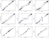 |
Fig. A.1 Comparison between the RVs measured on several lines for the primary (top panel), secondary (middle panel), and tertiary (bottom panel) components, respectively. |
References
- Baranne, A., Queloz, D., Mayor, M., et al. 1996, A&AS, 119, 373 [NASA ADS] [CrossRef] [EDP Sciences] [Google Scholar]
- Benaglia, P., Koribalski, B., & Albacete Colombo J. F. 2006, PASA, 23, 50 [NASA ADS] [CrossRef] [Google Scholar]
- Brott, I., de Mink, S. E., Cantiello, M., et al. 2011, A&A, 530, A115 [NASA ADS] [CrossRef] [EDP Sciences] [Google Scholar]
- Conti, P. S., Leep, E. M., & Lorre, J. J. 1977, ApJ, 214, 759 [NASA ADS] [CrossRef] [Google Scholar]
- Cox, N. L. J., Cami, J., Farhang, A., et al. 2017, A&A, 606, A76 [NASA ADS] [CrossRef] [EDP Sciences] [Google Scholar]
- De Becker M. 2007, A&ARv, 14, 171 [NASA ADS] [CrossRef] [Google Scholar]
- Duchêne, G., & Kraus, A. 2013, ARA&A, 51, 269 [Google Scholar]
- Gaia Collaboration, (Prusti, T., et al.) 2016, A&A, 595, A1 [NASA ADS] [CrossRef] [EDP Sciences] [Google Scholar]
- Gaia Collaboration, (Brown, A. G. A., et al.) 2018, A&A, 616, A1 [NASA ADS] [CrossRef] [EDP Sciences] [Google Scholar]
- Glebbeek, E., Gaburov, E., Portegies Zwart, S., & Pols, O. R. 2013, MNRAS, 434, 3497 [NASA ADS] [CrossRef] [Google Scholar]
- Gosset, E., Royer, P., Rauw, G., Manfroid, J., & Vreux, J.-M. 2001, MNRAS, 327, 435 [NASA ADS] [CrossRef] [Google Scholar]
- Heck, A., Manfroid, J., & Mersch, G. 1985, A&AS, 59, 63 [NASA ADS] [Google Scholar]
- Herbst, W., & Havlen, R. J. 1977, A&AS, 30, 279 [NASA ADS] [Google Scholar]
- Kharchenko, N. V., Piskunov, A. E., Röser, S., Schilbach, E., & Scholz, R.-D. 2005, A&A, 438, 1163 [NASA ADS] [CrossRef] [EDP Sciences] [MathSciNet] [Google Scholar]
- Kinoshita, H., & Nakai, H. 1999, Celest. Mech. Dyn. Astron., 75, 125 [NASA ADS] [CrossRef] [Google Scholar]
- Kozai, Y. 1962, AJ, 67, 579 [NASA ADS] [CrossRef] [Google Scholar]
- Le Bouquin, J.-B., Berger, J.-P., Lazareff, B., et al. 2011, A&A, 535, A67 [NASA ADS] [CrossRef] [EDP Sciences] [Google Scholar]
- Le Bouquin, J.-B., Sana, H., Gosset, E., et al. 2017, A&A, 601, A34 [NASA ADS] [CrossRef] [EDP Sciences] [Google Scholar]
- Lidov, M. L. 1962, Planet. Space Sci., 9, 719 [NASA ADS] [CrossRef] [Google Scholar]
- Mahy, L., Gosset, E., Sana, H., et al. 2012, A&A, 540, A97 [NASA ADS] [CrossRef] [EDP Sciences] [Google Scholar]
- Martins, F., Schaerer, D., & Hillier, D. J. 2005, A&A, 436, 1049 [NASA ADS] [CrossRef] [EDP Sciences] [Google Scholar]
- Naoz, S., Farr, W. M., Lithwick, Y., Rasio, F. A., & Teyssandier, J. 2011, Nature, 473, 187 [NASA ADS] [CrossRef] [Google Scholar]
- Prša, A., & Zwitter, T. 2005, ApJ, 628, 426 [NASA ADS] [CrossRef] [Google Scholar]
- Sana, H., de Mink, S. E., de Koter, A., et al. 2012, Science, 337, 444 [Google Scholar]
- Sana, H., Le Bouquin, J.-B., Mahy, L., et al. 2013, A&A, 553, A131 [NASA ADS] [CrossRef] [EDP Sciences] [Google Scholar]
- Sana, H., Le Bouquin, J.-B., Lacour, S., et al. 2014, ApJS, 215, 15 [NASA ADS] [CrossRef] [Google Scholar]
- Sanchez-Bermudez, J., Schödel, R., Alberdi, A., et al. 2013, A&A, 554, L4 [NASA ADS] [CrossRef] [EDP Sciences] [Google Scholar]
- Schneider, F. R. N., Langer, N., de Koter, A., et al. 2014, A&A, 570, A66 [Google Scholar]
- Skinner, S. L., Zhekov, S. A., Palla, F., & Barbosa, C. L. D. R. 2005, MNRAS, 361, 191 [NASA ADS] [CrossRef] [Google Scholar]
- Toonen, S., Hamers, A., & Portegies Zwart S. 2016, Comput. Astrophys. Cosmol., 3, 6 [CrossRef] [Google Scholar]
- Underhill, A. B. 1995, ApJS, 100, 433 [NASA ADS] [CrossRef] [Google Scholar]
- Walborn, N. R. 1971, ApJS, 23, 257 [NASA ADS] [CrossRef] [Google Scholar]
- Wilson, R. E., & Devinney, E. J. 1971, ApJ, 166, 605 [NASA ADS] [CrossRef] [Google Scholar]
The ((f*)) reports a spectrum with the N IV 4058 emission line stronger than the N III 4634–41 lines and a weak He II 4686 absorption line, the ((f+)) refers to a spectrum with medium N III 4634–41 emission lines, the weak He II 4686 line, and the Si IV 4089–4116 lines in emission, and the ((f)) means that the emission N III 4634–41 lines are weak and that the He II 4686 line is present in strong absorption (see Walborn 1971, for further details).
The BONNSAI web-service is available at http://www.astro.uni-bonn.de/stars/bonnsai.
All Tables
Top: Observed stellar parameters of the three components; bottom: Stellar parameters derived by BONNSAI.
All Figures
|
Fig. 1 RV curves of the inner system corrected for the presence of the tertiary component. Red dots give the RVs of the primary whilst the black ones indicate the secondary component. |
| In the text | |
|
Fig. 2 Left panel: RV curves of the outer system. Black dots represent the systemic velocities of the inner (P+S) system whilst the red ones represent the tertiary component. Right panel: relative astrometric orbit of the tertiary component in the outer system; the inner system is considered as fixed at (0,0). The periastron of the tertiary is represented by an open pentagon symbol. The observations are indicated in red and are accompanied with their error ellipses. |
| In the text | |
|
Fig. 3 Light curve of HD 150136 (black dots) and the PHOEBE best fit (red). The magnitude outside the eclipses has been set to 0 and lower luminosities correspond to negative values. |
| In the text | |
|
Fig. 4 Positions in the Hertzsprung–Russell diagram of the three components of HD 150136. Tracks are from Brott et al. (2011) computed with an initial rotational velocity of about 300 km s−1. |
| In the text | |
|
Fig. A.1 Comparison between the RVs measured on several lines for the primary (top panel), secondary (middle panel), and tertiary (bottom panel) components, respectively. |
| In the text | |
Current usage metrics show cumulative count of Article Views (full-text article views including HTML views, PDF and ePub downloads, according to the available data) and Abstracts Views on Vision4Press platform.
Data correspond to usage on the plateform after 2015. The current usage metrics is available 48-96 hours after online publication and is updated daily on week days.
Initial download of the metrics may take a while.