| Issue |
A&A
Volume 616, August 2018
|
|
|---|---|---|
| Article Number | A47 | |
| Number of page(s) | 19 | |
| Section | Planets and planetary systems | |
| DOI | https://doi.org/10.1051/0004-6361/201832804 | |
| Published online | 13 August 2018 | |
Migration of planets in circumbinary discs
Institut für Astronomie und Astrophysik, Universität Tübingen,
Auf der Morgenstelle 10,
D-72076
Tübingen,
Germany
e-mail: This email address is being protected from spambots. You need JavaScript enabled to view it.
; This email address is being protected from spambots. You need JavaScript enabled to view it.
Received:
10
February
2018
Accepted:
31
May
2018
Abstract
Aims. The discovery of planets in close orbits around binary stars raises questions about their formation. It is believed that these planets formed in the outer regions of the disc and then migrated through planet-disc interaction to their current location. Considering five different systems (Kepler-16, -34, -35, -38, and -413) we model planet migration through the disc, with special focus on the final orbital elements of the planets. We investigate how the final orbital parameters are influenced by the disc and planet masses.
Methods. Using two-dimensional, locally isothermal, and viscous hydrodynamical simulations, we first model the disc dynamics for all five systems, followed by a study of the migration properties of embedded planets with different masses. To strengthen our results, we apply two grid-based hydrodynamical codes using different numerics (PLUTO and FARGO3D).
Results. For all systems, we find that the discs become eccentric and precess slowly. We confirm the bifurcation feature in the precession period – gap-size diagram for different binary mass ratios. The Kepler-16, -35, -38, and -413 systems lie on the lower branch and Kepler-34 on the upper one. For systems with small binary eccentricity, we find a new non-monotonic, loop-like feature.
In all systems, the planets migrate to the inner edge of the disc cavity. Depending on the planet-disc mass ratio, we observe one of two different regimes. Massive planets can significantly alter the disc structure by compressing and circularising the inner cavity and they remain on nearly circular orbits. Lower-mass planets are strongly influenced by the disc, their eccentricity is excited to high values, and their orbits are aligned with the inner disc in a state of apsidal corotation.
In our simulations, the final locations of the planets are typically too large with respect to the observations because of the large inner gaps of the discs. The migrating planets in the most eccentric discs (around Kepler-34 and -413) show the largest final eccentricity in agreement with the observations.
Key words: hydrodynamics / methods: numerical / planets and satellites: formation / protoplanetary disks / binaries: close
© ESO 2018
1 Introduction
Following the first detection of a circumbinary planet with the Kepler space telescope, namely Kepler-16b, eight more binary star systems with a planet on a P-type orbit have been discovered1. All these systems show striking similarities. They are all very flat, meaning that the binary and the planet orbit are in the same plane, suggesting that these planets formed in a circumbinary disc aligned with the orbital plane of the central binary. Furthermore, in all systems, the innermost planet (so far only Kepler-47 is known to have more than one planet) is close to the calculated stability limit (Dvorak 1986; Holman & Wiegert 1999). This leads us to question where in the disc these planets formed. Two scenarios are possible: an in situ formation at the observed location, or a formation further outside the disc followed by radial migration of the planet through the disc to the observed location. Strong gravitational interaction between the binary and the disc, which leads to the excitation of spiral waves in the disc, makes an in situ formation unlikely (Pierens & Nelson 2007; Paardekooper et al. 2012; Meschiari 2012; Silsbee & Rafikov 2015), because for orbits close to the binary, destructive collisions between planetesimals are expected. The different alignment of their periapses lead to high relative impact velocities (Scholl et al. 2007; Marzari et al. 2008).
Therefore, it is believed that these circumbinary planets on orbits close to the stability limit were formed in the outer disc where the binary has less influence on the formation process. In order to reach their observed position, the planets then migrated through the disc to their present location either through type-I or type-II migration (Lin & Papaloizou 1986; Ward 1997; Nelson et al. 2000; Tanaka et al. 2002). This leads to the question of how this migration progress can be stopped at the right orbit.
Early work by Artymowicz & Lubow (1994) showed that through tidal interaction between the binary and the disc an eccentric inner gap in the disc forms. The structure of the gap, such as eccentricity and size, depends on disc parameters (viscosity, pressure) as well as on binary parameters (eccentricity, mass ratio). This was confirmed by various studies, which all showed an eccentric inner gap that slowly precesses in a prograde manner around the binary (Pierens & Nelson 2008, 2013; Kley & Haghighipour 2014, 2015; Lines et al. 2015; Miranda et al. 2017; Mutter et al. 2017a; Thun et al. 2017).
In several of these mentioned works, not only was the structure of the circumbinary disc investigated but also the migration of the planets. These simulations showed that the inner cavity of the disc constitutes a barrier for the migrating planet. The sudden drop of density produces a large positive corotation torque balancing the negative Lindblad torques responsible for the inward migration (Masset et al. 2006).
Pierens & Nelson (2013) modelled planets around the systems Kepler-16, Kepler-34, and Kepler-35. In their numerous simulations, they studied the impact of the discs’ pressure and viscosity onto the migration process of the planets. They found that the structure (size and eccentricity) of the inner cavity depends strongly on disc parameters, and therefore pressure and viscosity in the disc have a notable influence on the final orbital parameters, since the planets migrate to the edge of the cavity. Additionally, they not only simulated full grown planets but also migrating planetary cores. After the cores reached their final positions, gas accretion and dispersion of the gas disc were initiated. However, the final orbital parameters were comparable, independent of the migration scenario. For all studied systems, they found a set of disc parameters which produced the closest approximation to the observed values. But since they could not precisely reproduce the observed orbital parameters, they suggested more sophisticated disc models.
Kley & Haghighipour (2014) simulated planets around Kepler-38 in isothermal as well as radiative discs. Their radiative disc models include viscous heating, vertical cooling, and radiative diffusion in the midplane of the disc. In both models, the planet migrated as expected to the edge of the inner cavity. In their isothermal models, the inner gap was smaller than the observed orbit of the planet and therefore the planet migrated too close to the binary. However, this small inner cavity was a result of their overly large inner radius of the computational domain with Rmin = 1.67 abin. As shown in Thun et al. (2017), this inner radius should be of the order of the binary separation. In the radiative case, the viscous heating produced a disc with an even smaller inner cavity. Only by reducing the disc’s mass and its viscosity can a wider inner cavity and a final orbit of the planet close to the observed location be achieved.
In a second paper, Kley & Haghighipour (2015) simulated the evolution of planets in isothermal and radiative discs around the Kepler-34 system. Because of the high eccentricity of the Kepler-34 binary, a disc with a large eccentric inner cavity is created. Therefore, the planets stop at a position far beyond the observed location. Between the isothermal and radiative models, they could not find large differences. Additionally, they observed an alignment of the planets’ orbit with the precessing inner gap.
Mutter et al. (2017b) studied planets in self-gravitating circumbinary discs around the systems Kepler-16, -34, and -35. Their main result is that for very massive discs (five to ten times the minimum mass solar nebula, MMSN), the disc’s self-gravity can shrink the inner cavity which allows the planet to migrate further inward. This way they could achieve a better agreement between their simulations of the Kepler-16 and Kepler-34 systems and the observed values. In the case of Kepler-35b, the low mass of the planet prevented the planet from migrating close to the observed location.
In this paper, we revisit the evolution of embedded planets in circumbinary discs based on our new, refined disc models presented in Thun et al. (2017). To study the migration of fully formed planets through a circumbinary disc, we carried out two dimensional (2D), isothermal, and viscous hydrodynamical simulations. The binary parameters were chosen according to five selected Kepler systems. Table 1 gives an overview of binary and planet parameters of these systems. First, we simulated the circumbinary disc without the presence of a planet to obtain the dynamical properties of the inner cavity that we compare to our first study (Thun et al. 2017). In order to detect purely numerical features and strengthen our results, we used two grid codes, PLUTO and FARGO3D, that use different numerical methods, and compared their results.
For simulations with an embedded planet, we studied the evolution of the planet’s orbital elements as well as the planet’s impact on the disc. In these simulations, we varied the planet’s mass and the mass of the disc, in order to investigate the influence of the planet-to-disc mass ratio on the final orbital parameters of the planet.
The paper is organised in the following way. In Sect. 2, we describe the physical and numerical setup of our simulations. In Sect. 3, we discuss the disc structure prior to inserting the planet and compare it to our earlier study. In Sect. 4, we investigate how planets of different mass migrate through these circumbinary discs. We first discuss the general behaviour of migrating planets of different mass using the example of Kepler-38, and then comment on the other four systems. Our results are discussed and summarised in Sects. 5 and 6.
Circumbinary systems.
2 Model setup
2.1 Physical model
To model the migration of planets in circumbinary discs, we use 2D, isothermal, and viscous hydrodynamical simulations. For the disc model, we follow the setup described in Thun et al. (2017, Sect. 2). This means we solve the isothermal, vertically averaged Navier–Stokes equations with an external potential Φ on a polar grid (R, φ)2, centred at the barycentre of the binary.
We assume a locally isothermal temperature profile of T ∝ R−1 which corresponds to a disc with constant aspect ratio h = H∕R, where H is the height of the disc. In all simulations, we use h = 0.05. Turbulent viscosity in the disc is modelled through an α-parameter (Shakura & Sunyaev 1973), with α = 0.01. We have chosen these parameters to be consistent with our first paper but have run some exploratory simulations with smaller h and different α, we comment onthis in Sects. 3 and 5 below.
The external potential Φ has the following form:
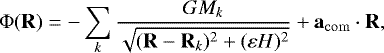 (1)
(1)
with k being an index running over both binary components and the planet (k ∈{A, B, p}). The subscripts A and B stand for the primary and the secondary star, and the subscript p for the planet. The smoothing factor εH is used to avoid singularities and to account for the correct treatment of a vertically extended three-dimensional (3D) disc in our 2D thin-disc approximation (Müller et al. 2012). In all our simulations, we use ε = 0.6. The disc height H is evaluated at the location of the cell H = hR. Since our coordinate system is located at the centre of mass of the binary, which is accelerated by the planet and the disc, we are not in an inertial reference system. This acceleration of the coordinate system, acom, gives rise to the indirect term acom ⋅R in Eq. (1), where acom is given by
![Mathematical equation: \begin{eqnarray*}\vec{a}_{\mathrm{com}} &=& \frac{ M_{\mathrm{A}} \vec{a}_{\mathrm{A}} +M_{\mathrm{B}} \vec{a}_{\mathrm{B}}} {M_{\mathrm{bin}}} \nonumber\\ &=& \frac{1}{M_{\mathrm{bin}}} \sum_{k\in\{\mathrm{A},\mathrm{B}\}} \frac{G M_{\mathrm{p}} M_k}{|\vec{R}_{\mathrm{p}}-\vec{R}_k|^3} (\vec{R}_{\mathrm{p}}-\vec{R}_k) \nonumber\\ &&+\frac{1}{M_{\mathrm{bin}}} \sum_{k\in\{\mathrm{A},\mathrm{B}\}} \int_{\mathrm{disc}} \frac{G M_k {\mathrm{\Sigma}}(\vec{R}') \,\mathrm{d} V'} {\left[ (\vec{R'}-\vec{R}_k)^2 +(\varepsilon H)^2\right]^{3/2}} (\vec{R}'-\vec{R}_k), \end{eqnarray*}](/articles/aa/full_html/2018/08/aa32804-18/aa32804-18-eq2.png) (2)
(2)
with themass of the binary Mbin = MA + MB. The first term in Eq. (2) is the acceleration of the centre of mass due to the planet and the second term is the acceleration due to the disc.
The equation of motion for the binary components and the planet is given by
![Mathematical equation: \begin{eqnarray*}\frac{\mathrm{d}^2 \vec{R}_k}{\mathrm{d}t^2} &= &- \sum_{\ell\neq k} \frac{G M_{\ell}}{|\vec{R}_k - \vec{R}_{\ell}|^3} (\vec{R}_k - \vec{R}_{\ell})\nonumber\\ &&+ \int_{\mathrm{disc}} \frac{G {\mathrm{\Sigma}}(\vec{R}') \,\mathrm{d} V'} {\left[(\vec{R}'-\vec{R}_k)^2+(\varepsilon H)^2\right]^{3/2}} (\vec{R}' - \vec{R}_k)\nonumber\\ &&- \vec{a}_{\mathrm{com}} \,. \end{eqnarray*}](/articles/aa/full_html/2018/08/aa32804-18/aa32804-18-eq3.png) (3)
(3)
Again the height of the disc is evaluated at the location of the cell H = hR′ (Müller et al. 2012). Equations (2) and (3) show the most general case in which the binary is accelerated by the planets and the disc. For disc-only simulations in Sect. 3, the back-reaction of the disc on the binary is not considered and therefore the disc contributions in Eqs. (2) and (3) are omitted.
2.2 Initial conditions
The initial disc density is given by
 (4)
(4)
where fgap models the expected cavity created by the binary (Artymowicz & Lubow 1994; Günther & Kley 2002)
![Mathematical equation: \begin{equation*} f_{\mathrm{gap}} = \left[1+\exp{\left(-\frac{R-R_{\mathrm{gap}}} {{\mathrm{\Delta}} R}\right)} \right]^{-1} \,, \end{equation*}](/articles/aa/full_html/2018/08/aa32804-18/aa32804-18-eq5.png) (5)
(5)
with Rgap = 2.5 abin, and ΔR = 0.1 Rgap. For the migration process, the total mass of the disc is an important quantity, since it directly influences the migration speed of the planet. In all our models, we choose an initial disc mass of Mdisc = 0.01 Mbin. With this choice, the reference surface density in Eq. (4) can then be calculated:
![Mathematical equation: \begin{align}M_{\mathrm{disc}} &= \int_0^{2\pi} \int_{R_{\mathrm{min}}}^{R_{\mathrm{max}}} {\mathrm{\Sigma}}(t=0) R \,\mathrm{d} R \,\mathrm{d} \varphi \\ &= 2\pi{\mathrm{\Sigma}}_{\mathrm{ref}} \int_{R_{\mathrm{min}}}^{R_{\mathrm{max}}} \left[1+\exp\left\{-\frac{\frac{R}{a_{\mathrm{bin}}} - 2.5} {0.25} \right\} \right]^{-1} \left(\frac{R}{a_{\mathrm{bin}}} \right)^{-1.5} R \,\mathrm{d} R \,. \end{align}](/articles/aa/full_html/2018/08/aa32804-18/aa32804-18-eq6.png) (6) (7)
(6) (7)
Introducing the dimensionless variable u = R∕abin (with umin∕max = Rmin∕max∕abin) gives
![Mathematical equation: \begin{equation*} M_{\mathrm{disc}} = 2\pi {\mathrm{\Sigma}}_{\mathrm{ref}} a_{\mathrm{bin}}^2 \underbrace{\int_{u_{\mathrm{min}}}^{u_{\mathrm{max}}} \left[1 + \exp\left\{-\frac{u-2.5}{0.25} \right\} \right]^{-1} u^{-0.5} \,\mathrm{d} u}_{= I(u_{\mathrm{min}}, u_{\mathrm{max}})}\,. \end{equation*}](/articles/aa/full_html/2018/08/aa32804-18/aa32804-18-eq7.png) (8)
(8)
Finally, thereference density is given in our case in code units3 with umin = 1 and umax = 40 by
 (9)
(9)
the integral I(1, 40) was evaluated numerically.
The initial radial velocity is set to zero uR(t = 0) = 0 and the initial azimuthal velocity is set to the local Keplerian velocity  .
.
2.3 Numerics
The grid spans from Rmin = 1 abin to Rmax = 40 abin in the radial direction with a logarithmic spacing and from 0 to 2π in the azimuthal direction with a uniform spacing. In all simulations, we use a resolution of 684 × 584 grid cells. At the inner edge, we use a zero-gradient boundary condition (∂∕∂R = 0) for density, radial velocity, and angular velocity Ωφ = uφ∕R. We further allow only outflow and no inflow into the computational domain. At the outer boundary, we set the azimuthal velocity to the local Keplerian velocity. For the density and radial velocity, we use a damping boundary condition in the range from (1 − f)Rmax to Rmax (with f = 0.1) as described in de Val-Borro et al. (2006). This means we damp a quantity x (here surface density Σ or radial velocity uR) to its initial value x0 according to
 (10)
(10)
where Δt is the current time-step, τ is the damping time scale and equal to one tenth of the orbital period at the outer boundary  . The damping function
  is a quadratic polynomial which fulfils the following conditions
 ![Mathematical equation: $\mathcal{P}([1-f] R_{\mathrm{max}}) = 0.0$](/articles/aa/full_html/2018/08/aa32804-18/aa32804-18-eq13.png) ,
,  and
and ![Mathematical equation: $\mathcal{P}'([1-f]R_{\mathrm{max}}) = 0.0$](/articles/aa/full_html/2018/08/aa32804-18/aa32804-18-eq15.png) . Therefore,
. Therefore,
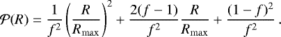 (11)
(11)
In the azimuthal direction, we use periodic boundary conditions.
For stability reasons, especially in the inner cavity where the density drops to very low values, we use a global density floor,
 (12)
(12)
in all our simulations. Without a density floor, some hydrodynamical codes, especially PLUTO, tend to produce negative densities and abort the calculation. Test simulations with lower floors did not show any differences in disc dynamics, but negative densities and code abortions occurred more frequently. Simulations with density floors higher than 10−6 Σref did not agree with the lower floor results, hence our choice for Σfloor.
In this paper, we use two hydrodynamical codes, namely PLUTO (Mignone et al. 2007)4 and FARGO3D (Benítez-Llambay & Masset 2016). For a quick overview of the numerical options used in our simulations see Thun et al. (2017, Sect. 3.1). Some details about the N-body solver implemented in PLUTO are shown in Appendix A.
FARGO3D uses an artificial von Neumann–Richtmyer viscosity to smooth out shocks. The artificial viscosity follows the ZEUS implementation (Stone & Norman 1992). The number of cells over which the shock is spread can be adjusted through a constant Cav (in the ZEUS paper, this constant is referred to as C2). FARGO3D sets this constant by default to Cav = 1.41. As discussedin Appendix B, to obtain a good agreement with PLUTO a lower artificial viscosity is needed. Therefore, we have chosen Cav = 0.5 for all FARGO3D simulations shown in this paper.
Figure 1 summarises our setup using the Kepler-38 system as an example. Displayed are various snapshots of the azimuthally averaged surface density in order to show that the density floor does not directly interfere with the disc evolution. The density snapshot is from a PLUTO simulation of Kepler-38 without a planet. The planets are then embedded at t = 10 000 binary orbits into the disc. In Table 2, all numerical and physical parameters which were not varied in our simulations are summarised.
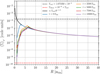 |
Fig. 1 Azimuthally averaged surface density at various times for the Kepler-38 system calculated with PLUTO. The blue curve shows the initial density distribution. The black vertical line marks the 1 abin location where the density would reach the reference density if we had not imposed an initial gap (blue curve). The dashed horizontal lines mark the reference density (in black) and the density floor (in red). |
Fixed numerical and physical parameters of our simulations.
3 Circumbinary disc structure
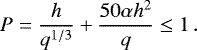
Before studying the evolution of embedded planets, we present our results on the dynamical behaviour of the circumbinary disc around the five systems under investigation. In Fig. 2, we display the time evolution over 40 000 orbits of thebinary of the disc’s precession period as well as the semi-major axis and the eccentricity of the disc’s gap. In the left column, results from PLUTO simulations are shown and in the right column FARGO3D results are presented.
The semi-major axis and eccentricity of the gap are calculated with the help of a fitted ellipse. The detailed fitting procedure is described in Thun et al. (2017, Sect. 5.1). The displayed data show some noise since we calculated the semi-major axis and eccentricity of the disc only every 100 binary orbits. The final estimates are time averages, starting at 6000 binary orbits (roughly the time when all discs reached a quasi steady state). The precession period is calculated in two ways: we searched for positive (π − δ → π + δ, δ ≪ 1) and negative (π + δ → π − δ) transitions in the ϖdisc-t-diagram (e.g., of a ϖdisc-t-diagram see Fig. 12 below). The time between two subsequent positive (× in Fig. 2) or negative (+ in Fig. 2) transitions gives the precession period of the gap, which is shown in the first row of Fig. 2 ordered by their number of occurrence. To obtain a better estimate, we averaged over all periods after the discs reached a quasi-steady state, which happens after about 6000 binary orbits. The overall agreement between the results obtained with PLUTO and FARGO3D is very good; we discuss some notable differences below.
Considering the different binary eccentricities in our systems, as noted in Table 1, we can place them in a Tprec versus agap diagram; see Fig. 3. In a previous study, we discovered a bifurcation with two separate branches depending on the binary eccentricity (Thun et al. 2017, Sect. 5.2). In that study we found that on the lower branch, starting with circular binaries, the precession period and gap size decrease for increasing binary eccentricities. The minimum gap size and precession period are reached at a critical binary eccentricity of ecrit≈ 0.18. From there, the upper branch starts on which both quantities increase for increasing binary eccentricities. The vertical axis in Fig. 3 has been rescaled using the factor
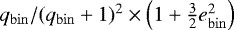
 (13)
(13)
to account for the different binary mass ratios and eccentricities. As shown in Thun et al. (2017, Appendix B) the precession period of the disc gap is comparable to the precession period of a single particle around a binary,
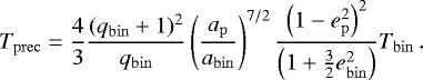 (14)
(14)
Our scaling factor does not include the gap eccentricity term  , in order to allow for a clear relation between binary and individual disc properties, here Tprec versus agap. From Fig. 4, it is, in principle, possible to construct a relation between egap and agap and add this to the scaling in Fig. 3. Using egap in the scaling for Fig. 3 does not change it qualitatively, only the exponents are different then.
Using this scaling, the numerically obtained disc parameters can be placed into the diagram for all systems, which lie indeed very close to the discovered bifurcation curve of Thun et al. (2017). While Kepler-16 and Kepler-35 are located close to the branching point, the systems Kepler-38 and Kepler-413lie on the lower branch. The Kepler-34 system, which has a very large gap with a slow precession, is located at the end of the upper branch in Fig. 3.
Fits to the upper and lower branch data points show that the scaled precession period is proportional to  on the lower branch and
  on the upper branch. These exponents are lower than the exponent 7∕2 expected from the test particle precession period relation, Eq. (14). This deviation represents the fact that gap’s dynamical behaviour is determined by hydrodynamical effects and does not fully behave like a free particle around a binary.
To generate Fig. 3, we did not use the data from Thun et al. (2017) but generated all points for the different binary massratios and eccentricities using our new improved numerical setup as described above, in particular a smaller Rmin. The red points in the figure are all calculated for the Kepler-16 binary mass ratio of qbin = 0.29, and the green and blue bullets correspond to mass ratios of qbin = 0.60 and qbin = 0.90. We also set up simulations series for these high mass ratios since Kepler-34 also has a high mass ratio of qbin = 0.97. For binary eccentricities, ebin ≥ 0.06, we observe the same behaviour as in our earlier study: upon increasing ebin, the points move along the lower branch towards smaller agap and Tprec until the critical value ecrit ≈ 0.18 is reached, from which both Tprec and agap increase with increasing ebin. However, for binary eccentricities smaller than ebin = 0.06, we observe a new phenomenon. Starting from circular binaries, the gap size as well as the precession period first increase until a maximum is reached for ebin = 0.06; see inlay inFig. 3. Increasing the binary eccentricity past ebin = 0.06 leads to smaller gaps and lower precession periods again, following the known trend. From ebin = 0.0 to ebin = 0.08, a loop-like structure is created. In Thun et al. (2017), we did not notice this loop-type behaviour for small ebin because we only simulated ebin = 0.0 and ebin = 0.08 and no values in between. Using a smaller Rmin = abin and a better coverage of small ebin values allowed us to discover this new, complex behaviour. Although this constitutes a very exciting new finding, we defer further investigation to a subsequent study. We only note here that, as shown in the inlay of Fig. 3, this loop-like structure is also present for higher mass ratios of qbin =0.60 and qbin = 0.90 confirming the generality of our results.
Figure 4 shows the correlation of gap eccentricity and gap size for different binary eccentricities as well as different binary mass ratios. Discs around binaries with eccentricities close to zero create the most eccentric gaps, while binaries with eccentricities close to the branching point have the smallest and least eccentric gaps. High eccentric binaries create the largest gaps which are also highly eccentric.
Figures 3 and 4 have been generated from models using our standard aspect ratio and viscosity. Exploratory simulations with different h (0.03, 0.04) and α (0.001, 0.05) show the same trend as described in Thun et al. (2017). Increasing the viscosity leads to smaller, more circular gaps with shorter precession periods, and the same trend holds for smaller aspect ratios. Due to the neglect of the disc backreaction on the binary for these simulations without embedded planet, the results displayed in Figs. 3 and 4 refer to the zero disc mass limit. In our case of small disc mass (Mdisc = 0.01 Mbin) this is a very good approximation. For a test simulation for our standard model (Kepler-38), which included disc backreaction, the change in ebin over the first 50 000 binary orbits was less than 2%.
Table 3 summarises the gap properties of the five systems as calculated using the PLUTO code. Although the systems studied in this paper have mass ratios different from qbin = 0.29, which is the value of Kepler-16 investigated in Thun et al. (2017), the general behaviour is in good agreement with our earlier study. The most circular system (Kepler-413) produces the most eccentric gap, with an eccentricity of egap= 0.43, while the largest gap is formed by the most eccentric binary (Kepler-34), which also has the longest precession period of Tprec = 4000 Tbin. Systems close to the branching point (Kepler-16 and Kepler-35) have the smallest gaps with the shortest precession periods. Kepler-35 has the shortest precession period of Tprec = 1079 Tbin, since the mass ratio of Kepler-35is, with qbin = 0.91, almost equal to one, and higher mass ratios lead to shorter precession periods (Thun et al. 2017). Since the mass ratio does not change the gap size significantly, Kepler-16, which has an eccentricity closer to the critical eccentricity than Kepler-35, has the smallest gap of all systems considered in this paper. As already seen in our earlier study we find that the size of the gap is directly correlated with the precession period of the gap, for all systems under investigation. This behaviour is expected from single particle trajectories and supported by the used scaling for Tprec in Fig. 3. Comparing with Table 1, one can see that the two systems with the highest gap eccentricity (Kepler-34 and -413) also possess the planets with the highest eccentricity.
Concerning the outcome of the different numerical methods, the best agreement between PLUTO and FARGO3D is obtained for Kepler-38 and -413; both systems are on the lower branch and far away from the branching point. For our two systems close to the branching point (Kepler-16 and -35), FARGO3D produces slightly higher precession periods than PLUTO, however the gap size and eccentricity match very well. The largest deviations between the two codes can be seen for the Kepler-34 system, which produces the largest gap. Here, the precession period deviates by roughly ten percent and the gap size by five percent between the two codes.
Overall, the static disc parameters (gap size and eccentricity) are in good agreement between the two codes for all systems. However, for the dynamical parameter (precession period of the gap) the codes can deviate slightly, depending on the observed system. This could be a consequence of the very low precession rate, especially for Kepler-34, where the gap is nearly stationary with respectto the inertial frame.
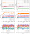 |
Fig. 2 The precession period, semi-major axis, and eccentricity of the disc gap vs. time, for our five different systems. Disc models on the left are calculated with PLUTO and disc models on the right are calculated with FARGO3D. The precession period, Tprec, in the first row is given in terms of the corresponding period number. The horizontal lines indicate the time average starting from 6000 binary orbits, roughly the time when the discs reached a quasi-steady state. See the text for an explanation of the meaning of the + and × signs in the first row. |
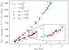 |
Fig. 3 Precession period of the inner gap, scaled by the factor |
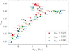 |
Fig. 4 Gap eccentricity plotted against the semi-major axis of the gap. Different bullets correspond to numerical results for different binary eccentricities whereas different colours stand for different binary mass ratios. The five different Kepler systems considered in this paper are marked by the black stars. |
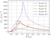 |
Fig. 5 Azimuthally averaged density profiles after 10 000 binary orbits for the five different Kepler systems. The dots mark the initial planet position. |
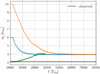 |
Fig. 6 Time evolution of the semi-major axis of a mp = 0.384 Mjup planet with different initial positions in a circumbinary disc around the Kepler-38 system. The black line shows the observed position of the planet. |
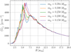 |
Fig. 7 Azimuthally averaged density profiles for the Kepler-38 disc with embedded planets after 12 000 binary orbits. The planets were held on a fixed orbit (ap = 6.0 abin) for 2000 binary orbits. |
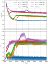 |
Fig. 8 Orbital elements of migrating planets in a circumbinary disc around the Kepler-38 system with different masses. Top panel: semi-major axis of the planet. Bottom panel: eccentricity of the planet. The black lines show the observed values, for the eccentricity only an upper limit is known. The upper mass limit for Kepler-38b is mp = 0.384 Mjup. |
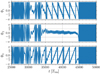 |
Fig. 9 Three out of eleven resonant angles for the mp = 0.150 Mjup case. While the resonant angles Φ1 and Φ3 cover the fullrange from 0 to 2π the resonant angle Φ2 librates around zero during the resonant phase of the planet (from t = 34 000 Tbin to t = 45 000 Tbin). The resonant angles Φ3 to Φ11 also cover the full range from 0 to 2π but are not shown for clarity. |
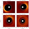 |
Fig. 10 Structure of the inner disc for the Kepler-38 system. The surface density is colour-coded, since the absolute density values are not important for the disc structure we omit the density scale for clarity (brighter colours mean higher surface densities). The top-left panel shows the circumbinary disc after 10 000 binary orbits before the planet is inserted. The remaining three panels show the disc structure with an embedded planet of varying mass after 76 500 binary orbits. The binary components and the planets are marked with black dots. The direction of pericentre of the secondary (green), the planet (blue), and the disc (orange) are marked by the arrows. Additional fitted ellipses to the central cavity are plotted in dashed white lines and the actual orbit of the planet is shown as dashed blue line. Using the fitted ellipses, the size and eccentricity of the disc gap, shown in the upper left edge of each panel, are calculated at the same time. As we saw in Fig. 2 these quantities show small variations in time around some average value. |
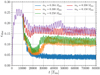 |
Fig. 11 Time evolution of the inner disc eccentricity for Kepler-38. Planets of different mass were introduced into the simulations at 10 000 binary orbits on circular orbits and allowed to migrate through the disc after 12 000 binary orbits. |
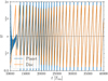 |
Fig. 12 Time evolution of the pericentres of a planet with mass mp = 0.250 Mjup (blue) and the disc (orange) for Kepler-38. Until t = 12 000 Tbin the planet ison a fixed circular orbit and therefore the pericentre is not well defined. After switching on the back-reaction onto the planet, its orbit soon becomes aligned with the inner precessing cavity of the disc. |
Disc properties of the five systems obtained with PLUTO simulations.
4 Planets in circumbinary discs
In this section, we describe the evolution of planets in the circumbinary discs around our five systems under investigation. In the first part, we give an account of the general behaviour using the sample system Kepler-38, and then describe the specifics of the other systems below. Before inserting the planets into the discs, we evolved the circumbinary discs for all systems without a planet for 10 000 binary orbits such that a quasi steady state was reached; see Fig. 2. We then inserted the planet into the disc and kept it on a fixed circular orbit for another 2000 binary orbits, so that the disc could adjust to the presence of the planet. After that we switched on the back-reaction of the disc onto the planet, meaning the planet was allowed to migrate freely through the disc. We also switch on the back-reaction of the disc onto the binary which leads to a very slow increase of the binary eccentricity and a slow decrease of the binary separation, accompanied with a small reduction of the binary orbital period, Tbin. When we refer to Tbin, we always mean the initial, unperturbedbinary period  , calculated using the observed values summarised in Table 1. The back-reaction from the planet and the disccauses also a precession of the binary, which is much slower compared to the precession of the inner gap and theplanet’s orbit. The azimuthally averaged density profiles of the disc for all five systems after 10 000 Tbin is displayed in Fig. 5 together with the initial positions of the embedded planets.
When simulating planets with the observed mass for our five systems, we found two regimes with different dynamical behaviour of the planet. To trigger these two regimes in all systems, we have chosen planet-to-binary mass ratios q from q ≈ 10−4, approximately the observed planet-to-binary mass ratio in the Kepler-34 system (light case), up to q ≈ 3.6 × 10⁻⁴, approximately the observed planet-to-binary mass ratio in the Kepler-16 system (massive case). This range of mass ratios leads in the case of Kepler-34, -35, and -413 to planets which are way more massive than the observed planet. Nonetheless, we simulated these high-mass planets to explore if the two regimes (here the massive case) can also be triggered in those systems as well.
In this section, all presented results were obtained by PLUTO simulations. In Appendix B, we compare PLUTO and FARGO3D simulations of a circumbinary disc with an embedded planet.
4.1 Kepler-38
In this section, we use the Kepler-38 system as our reference system to illustrate the general behaviour of a planet embedded in a circumbinary disc. We have chosen Kepler-38 because for this system the best agreement between PLUTO and FARGO3D is obtained. Furthermore, we can compare our results directly with Kley & Haghighipour (2014) who also looked at Kepler-38 applying a different numerical setup. They used an initial density slope proportional to R−0.5 whereas we use Σ ∝ R−1.5 in this study. However, test calculations have shown that the initial density profile has no influence on the final quasi-steady state. A more crucialdifference is the position of the inner boundary. Kley & Haghighipour (2014) used an inner radius of Rmin = 1.67 abin. However, as we have shown in Thun et al. (2017) this radius is too large because it does not allow the full disc dynamics todevelop and results in very small and circular gap edges. For this reason, we have chosen here Rmin = abin for all systems.
4.1.1 Initial planet position
In a first series of simulations, we investigate how the final stopping position of the planet depends on its initial starting position. We simulated a Saturn-like planet with a mass of mp = 0.384 Mjup, which is theupper mass limit for Kepler-38b. Initially, we placed the planet at three different locations inside the disc. The red curve in Fig. 5 shows the density profile for Kepler-38, and the red symbols mark the three initial locations of the planet. The outermost starting point is at Rp (t = 0) = 10 abin, beyond the density maximum, which is produced by the binary-disc interaction. The second starting point was placed just inside of the density maximum at 6.0 abin, and finally the last starting point was placed at the observed location 3.096 abin.
Figure 6 shows the time evolution of the semi-major axis of the planet for the three initial starting points. Independently of its initial position, the planet migrates through the disc until it stops at a distance of approximately 3.98 abin = 0.597 au. The observed semi-major axis of Kepler-38b is aobs = 0.4644 au. For the two outer starting points, the planet migrates inward until it reaches the edge of the inner cavity, which is created by the gravitational interaction of the binary on the disc. This behaviour is expected since at this point the negative Lindblad torques, responsible for inward migration, are balanced by the positive corotation torques and the planet migration comes to rest (Masset et al. 2006). If we initially place the planet at the observed location, which lies inside of the cavity, then the planet starts to migrate outward to the edge of the disc where the torques are again in balance (green curve in Fig. 6). Such an outward migration of a planet when starting inside of the cavity has been found for the Kepler-34 system by Kley & Haghighipour (2015). It is caused by the transfer of positive angular momentum to the planet when interacting with the eccentric inner disc.
The independence of the final planet position from its initial conditions suggest that the planet is subject to type I migration, since the disc is hardly perturbed. To investigate this further, we calculated the gap open criterion by Crida et al. (2006)
 (15)
(15)
For our range of planet-to-binary mass ratios and our fixed disc parameters (h = 0.05, α = 0.01) the gap open criterion is not met, confirming the type I migration regime. Even very high-mass planets cannot open a full gap (P ≈ 4); they only produce a small dip in the density profile of the disc. This can be seen in Fig. 7 for the case of Kepler-38.
Our findings are in good agreement with Kley & Haghighipour (2014) who also did not find a dependence of the final planet position on the initial position. However, in their simulations, the planet migrated further in and stopped at ap = 0.436 au, which is very close to the observed location. However, this extended inward motion was an artefact of the incorrect location of the inner boundary of the grid for which an overly large inner radius was chosen.
Since the initial location of the planet does not impact its final stopping position, we always place the planet for Kepler-38 and the other systems slightly inside the peak density to save some computational time. The azimuthally averaged density profiles of all systems after 10 000 binary orbits together with the initial planet positions can be seen in Fig. 5.
4.1.2 Variation of planet mass
In this section, we investigate the influence of the planet mass on the migration process. In Fig. 8, we display the time evolution of the semi-major axis (top panel) and the eccentricity (bottom panel) of planets with different masses which range here from mp =0.150 Mjup to mp = 0.384 Mjup, the upper limit of the observed planet. One can see that, depending on the mass of the planet, two eccentricity states exist and that the migration path of the planet through the disc differs for those two states. The heaviest planet (with mp = 0.384 Mjup) migrates smoothly to its final position and its eccentricity remains very low. The lighter planets start migrating inwards until they reach a turning point (the lighter the planet is, the earlier this point is reached). From there on, the planet undergoes a fast and short period of outward migration, during which the eccentricity of the planet is increased to ≈ 0.20−0.22. This increase in eccentricity does not depend strongly on the planet mass. After the eccentricity is increased, the planets migrate towards the binary very slowly, compared to the first inward migration phase.
Before discussing the origin of these different migration scenarios, we focus briefly on a special behaviour of the lightest planet with mass mp = 0.150 Mjup. At around t ≈ 34 000 Tbin into the evolution, one notices an additional increase in eccentricity of the planet while the migration seems to stall at around ap = 4.93 abin; see purple curves in Fig. 8. This phase of constant semi-major axis and increase of eccentricity lasts until 45 000 binary orbits. During this phase, we find for the quotient of the planet’s period to the binary period, Tp ∕Tbin ≈ 11.2, suggesting a possible capture into the 11:1 resonance between the planet and the binary as the reason for this behaviour of the planet. The position of this 11:1 resonance lies at a11:1 = 4.93 abin. To check for this idea, we calculated the k resonance angles, which are for a general p:q resonance with p > q given by
 (16)
(16)
with q ≤ k ≤ p. Here, λp and λbin are the mean longitudes of the planet and the binary and ϖp and ϖbin the longitudes of periapse. The planet and the binary are in a p:q resonance when at least one resonant angle Φk does not cover the full range from 0 to 2π (Nelson & Papaloizou 2002; Kley & Haghighipour 2014). In our case, Φ2 librates around zero and all other angles cover the full range. Figure 9 shows the first three resonant angles as a selection to illustrate the behaviour of the librating angle and angles which cover the full range. This confirms that the planet is indeed captured in a 11:1 resonance with the binary. After 45 000 binary orbits, the planet is kicked out of this resonance, its semi-major axis increases shortly and its eccentricity decreases to the value before the resonant capture occurred. After this short resonant capture, the planet resumes its slow inward migration, similarly to the other planets. As seen in Fig. 9, previous to this extended phase of being engaged in the 11:1 resonance, there was a brief capture into the same resonance at t ≈ 31 000 Tbin.
Coming back to the interaction of the planets with the disc, the impact of an embedded planet has on the ambient disc with constant aspect ratio and constant turbulent viscosity depends on its mass. For the most massive planet, we found that the inner disc became more circular with a reduced size of the inner gap. This allowed the planet to migrate further inward towards the binary. Lighter planets cannot alter the disc structure in such a strong way due to the reduced gravitational impact. The change of the inner disc structure in the presence of a planet is illustrated in Fig. 10. This figure shows the 2D surface density for three different planet masses as well as the disc structure prior to inserting the planet (top left panel). The white dashed lines show the fitted ellipses to the inner cavity. One can immediately see how the size and eccentricity of the gap decrease with increasing planet mass. Another observation is that the final position of the planet is always close to the edge of the gap. The dashed blue lines show the orbit of the planet, which lies in all cases just outside the fitted ellipse. Going from the upper left panel to the lower right panel, we see the clear trend that eccentricity and semi-major axis of the gap is decreasing as the planet mass is increased.
A more quantitative image of this behaviour can be seen in Fig. 11, which shows the time evolution of the inner disc eccentricity. The disc eccentricity and the disc pericentre (in Fig. 12) are calculated according to Thun et al. (2017, Sect. 2.5) within a limited radial interval [R1, R2], where R1 = Rmin and R2 is chosen differently for each system such that it lies at a point slightly outside the density maximum. For the five systems considered in this paper, we have chosen R2 = {7.0, 12.0, 7.0, 7.0, 9.0} abin (compare to Fig. 5). For the first 10 000 binary orbits, no planet is present in the simulations and the disc eccentricity rises to about edisc ≈ 0.25. After 10 000binary orbits, the planet is introduced into the simulation, and after 12 000 binary orbits, the planet is allowed to migrate through the disc. At the moment the planet is embedded, the disc’s eccentricity decreases; the heavier the planet is, the more abrupt the decrease. For the light planets, except the planet with mass mp = 0.150 Mjup, the disc “pushes” back, increasing its eccentricity again. From this point, the inner disc eccentricity stays more or lessconstant. This push-back phase coincides with the outward migration phase of the planet (see Fig. 8). Interestingly, this increase of the disc eccentricity only increases the planet’s semi-major axis but notthe eccentricity of the planet. In the case of the massive planet, the disc is not able to “push back”, as it is not massive enough, and the disc eccentricity continues to decrease smoothly to a final value of edisc = 0.043.
As indicated by the arrows in Fig. 10, which mark the pericentre of the secondary (green), the planet (blue), and the disc(orange), the pericentre of the disc and the planet are aligned in the case of the light planets. For the massive planet, no such alignment is observed; the similar directions of disc and planet pericentre at this snapshot are coincidental. Also, the definition of a unique pericentre becomes difficult in the case of massive planets, because the planet orbit and the disc gap have an eccentricity close to zero. The time evolution of the directions of pericentre for disc and planet is shown in Fig. 12 for the mp = 0.250 Mjup case. The orbital alignment between disc and planet is achieved during the first 10 000 binary orbits after releasing the planet.
Kley & Haghighipour (2015) and Mutter et al. (2017b) also found this alignment of planet orbit and inner disc cavity for the Kepler-34 system.
4.1.3 Variation of disc mass
As we have seen in the previous section, the planet can, depending on its mass, modify the disc structure. To investigate now the influence of the disc mass on this behaviour, we set up simulations with a different disc mass before introducing the planet into the disc. In all our models, we started with an initial disc mass of Mdisc = 0.01 Mbin. Since material can leave the computational domain through the inner open boundary, the disc will lose mass over time. After 10 000 binary orbits, before adding the planet to the simulation, the disc in the standard model has a mass of M10000 ≡ Mdisc(t = 10 000 Tbin) = 0.008967 Mbin. For two different planet masses, we increased or decreased the disc mass and followed the evolution of the embedded planets. Due to the local isothermal assumption, the neglect of the disc self-gravity and the independence of the potential of the surface density (the back-reaction of the disc onto the binary is not yet switched on, this means the disc terms in Eqs. (2) and (3) are neglected), the mass of the disc can be rescaled without changing itsdynamics. The set of models using this disc mass rescaling is summarised in Table 4.
The top part of Table 4 gives an overview of the planet-disc mass ratio of two models, using the standard disc mass. As seen in the previous section, the planet with mass mp = 0.384 Mjup, which was the most massive planet, could alter the disc structure, whereas a planet with mass mp = 0.200 Mjup could not. The bottom part of Table 4 shows the planet-disc mass ratio for models with increased or decreased disc mass. For the mp = 0.384 Mjup model, we increased the disc mass by a factor of three so that the planet-disc mass ratio is now comparable to the mp = 0.200 Mjup case with standard disc mass. Therefore, we expect that now the massive planet cannot alter the disc structure and will end up in a state with high eccentricity. In the case where mp = 0.200 Mjup, we decreased the disc mass by a factor of one half to increase the disc-planet mass ration to the regime where the planet can alter the disc. In this case, the planet should migrate smoothly inwards and end up in a state with very low eccentricity.
The results of these simulations are summarised in Fig. 13. The colours for the simulations with the standard disc mass are identical to Fig. 8. The migration speed of the mp = 0.384 Mjup planet in the disc with triple mass is very rapid compared to the standard disc. Since the migration speed is directly proportional to the disc mass, this behaviour is expected. This fast inward migration period lasts for approximately 552 binary orbits, during which the eccentricity of the planet is increased to ep = 0.184. Following that phase, the planet migrates again outward for a very short period of time, as already seen for low-mass planets in the standard disc. After that short period of outward migration, the planet resumes its inward migration but with a very low speed compared to the initial inward migration period. This is probably due to the high eccentricity of the planet. At around 80 000 binary orbits, the planet is captured in a 9:1 resonance with the binary, which increases its eccentricity further to a final value of ep = 0.273. The capturein resonance is confirmed by analysing the resonant angles; see Eq. (16). Again, Φ2 librates around zero, while all the other angles circulate and cover the full range. Although the planet is in resonance with the binary its semi-major axis still decreases slowly. This is due to the fact that the binary separation decreases faster than in the standard case due to the three times increased disc mass. This time, the planet’s orbit is aligned with the precessing inner gap of the disc.
The mp = 0.2 Mjup planet in the standard-disc-mass case is captured in a 8:1 resonance with the binary after t = 110 000 Tbin. For the reduced-disc-mass case (last row in Table 4), the mp = 0.2 Mjup planet migrates slowly through the disc with no turning point. At the beginning, the eccentricity of the planet is close to zero, as expected, because due to the reduced disc mass the planet is now able to circularise the disc. Additionally, the orbit of the planet is not aligned with the inner gap. At around 30 000 binary orbits, the eccentricity increases and starts to fluctuate around ep = 0.10 on a long timescale.
After having described the main features of planet migration in circumplanetary discs for the Kepler-38 system, we turn now to the other four systems. As before, we run the disc with initially 10−2 Mbin without a planet for 10 000 Tbin and then embed planets of different masses. For the first 2000 Tbin the planet is fixed at its orbit, then released and evolved for about 70 000 Tbin. The final orbital parameters for the planets with the observed mass can be found in Table 5, together with the observed values.
Planet mass mp, disc mass Mdisc and the ratio q = mp∕Mdisc for models using different disc masses.
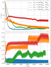 |
Fig. 13 Time evolution of semi-major axis (top) and eccentricity (bottom) of planets with different mass in discs of different mass, for the Kepler-38 system. |
Final orbital parameters of the embedded planets using the observed mp for the five systems investigated, calculated using the PLUTO simulations.
4.2 Kepler-16
To study the evolution of planets in the Kepler-16 system, we performed simulations with different planet masses starting from the observed mass of mp = 0.333 Mjup down to a mass of mp = 0.150 Mjup. Figure 14 shows the time evolution of the semi-major axis (top) and eccentricity (bottom) of the different planets. As seen in the eccentricity evolution, there are two distinct states, similar to the Kepler-38 case. The eccentricity of the more massive planets is not excited and remains close to zero, oscillating around ep = 0.029, whereas the eccentricity of the lighter planets is increased during the first 8000 binary orbits, after releasing the planets, to a mean value of ep = 0.15. These two states also differ in their alignment of the orbits with the inner gap of the disc. The lighter planets with high eccentricity end up in a state with aligned orbits, whereas no such alignment can be observed for the heavier planets. In the semi-major axis evolution, these two states are not as clearly visible as in the Kepler-38 system. Nonetheless, a difference between the massive and light planets can be observed. Heavy planets migrate smoothly through the disc, whereas the semi-major axis evolution of the lighter planets shows more noise. The massive planets start to migrate inwards smoothly, as expected from the Kepler-38 case. This phase smoothly transitions to a slow outward migrating phase, as seen also in long time simulations of Kepler-38 (see blue curve in Fig. 13). The lighter planets have also a period of outward migration, but this period is very short and followed by a second period of inward migration, as in the Kepler-38 case. The migration speed during this second inward period is far lower than during the first phase. The light planets show the same general behaviour as in the Kepler-38 case and they even migrate further in than their heavier counterparts. One reason for this could be that Kepler-16 has the smallest gap with the lowest eccentricity and therefore the circularising effect of heavier planets is not as important as in the other systems. This also implies that the increase of eccentricity is connected to the alignment of the planets orbit with the disc gap.
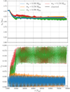 |
Fig. 14 Orbital elements of migrating planets in a circumbinary disc around the Kepler-16 system with different masses. Top panel: semi-major axis of the planet. Bottom panel: eccentricity of the planet. The black lines show the observed values. The observed mass of Kepler-16b is mp = 0.333 Mjup. |
4.3 Kepler-34
For the Kepler-34 system, we simulated planets with masses from the observed mass of mp = 0.220 Mjup up to mp = 0.800 Mjup. Figure 15 gives an overview of the orbital elements (semi-major axis and eccentricity) of the simulated planets. In all cases, we observe nearly the same migration behaviour, first a fast inward migration followed by a short period of outward migration. After that, the planets are relatively soon (after around 40 000 Tbin) parked in their final position. In all cases, the final orbits of the planets are relatively eccentric, with ep well above 0.2, and they are fully aligned with the eccentric gap of the disc and precess at the same rate. Although the massive planets can circularise the inner cavity slightly, this effect is not strong enough, because of the large and highly eccentric initial gap (agap = 6.99 abin, egap = 0.4). For the planet with the observed mass of mp = 0.220 Mjup we find a final semi-major axis of ap = 7.77 abin and an eccentricity of ep = 0.31 (see also Table 5).
In their study of the planet in Kepler-34, Kley & Haghighipour (2015) observed the same migration behaviour as we find here: a fast inward migration to the edge of the inner cavity. They find in their simulations a smaller semi-major axis of ap = 6.1 abin and a comparable eccentricity of ep = 0.3. One reason for the difference in the planets semi-major axis could be again the position of the inner computational boundary. Kley & Haghighipour (2015) used a value of Rmin = 1.47 abin, which is too large (Thun et al. 2017). Furthermore, they use a uniformly spaced grid in the R-direction with only 256 cells. Therefore, their resolution in the inner part of the computational domain is very low, which could be another reason for the observed differences, but they also found an alignment of the planet’s orbit with the inner eccentric cavity.
For Kepler-34, Mutter et al. (2017b) found for their one- and two-MMSN disc models (our disc mass lies in between these two) a final semi-major axis of ap ≈ 8.7 abin and an eccentricity of ep = 0.25−0.3, in relatively good agreement with our results. Furthermore, they also find an alignment of the planet’s orbit with the disc cavity. They mention this alignment only in the case of a planetary core with very low mass, but since they see no big difference between the full mass planet and the planetary core, we assume that this alignment also happens in the case of the fully grown planet.
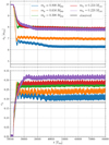 |
Fig. 15 Orbital elements of migrating planets in a circumbinary disc around the Kepler-34 system with different masses. Top panel: semi-major axis of the planet. Bottom panel: eccentricity of the planet. The black lines show the observed values. The observed mass of Kepler-34b is mp = 0.220 Mjup. |
4.4 Kepler-35
For Kepler-35, we studied the migration of planets starting from the observed mass mp = 0.127 Mjup up to mp = 0.550 Mjup. Figure 16 shows results of simulations with the different planet masses. The two most massive planets with mp = 0.550 Mjup and mp = 0.500 Mjup show the typical behaviour of massive planets, as already discussed for the other systems. Their eccentricity remains low and they do not aligntheir orbit with the precessing inner gap of the disc.
The eccentricity of planets with masses from mp = 0.300 Mjup to mp = 0.450 Mjup become excited to a mean value of about 0.15. The planet with mass mp = 0.300 Mjup ends up in a 9:1 resonance with the binary after 55 000 binary orbits, and therefore its eccentricity is increased further. This planet also shows the general migration behaviour of lighter planets, as seen for the other systems. This behaviour is not as clearly visible for the planets with masses mp = 0.400 Mjup and mp = 0.450 Mjup, since they are both captured in a 8:1 resonance with the binary after t ≈ 23 000 Tbin.
The planet with the observed mass of mp = 0.127 Mjup shows a behaviour not yet observed for the other systems. Its eccentricity is increased fast to a value slightly below 0.25. After roughly 44 000 binary orbits, its eccentricity drops rapidly to a value below 0.15. This drop is also visible in the semi-major axis of the planet. A FARGO3D comparison simulation with a planet of this mass shows the same behaviour, but at a later time. The fast drop in eccentricity happens there at roughly 59 000 binary orbits. Besides this time shift, the PLUTO and FARGO3D curves for the semi-major axis and the eccentricity have a very similar evolution. For both codes, the drop in eccentricity (for mp = 0.127 Mjup) happens when the planet crosses ap ≈ 4.75 abin. Since in the case of FARGO3D, the planet migrates slower, it needs more time to reach this point. A reason for this behaviour could be thevery low mass of the planet compared to the disc in this case. Therefore, the influence of the disc on the planet is very high, and the disc eccentricity drops simultaneously. The final orbital parameters of the migrated planet are summarised in Table 5.
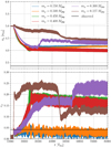 |
Fig. 16 Orbital elements of migrating planets in a circumbinary disc around the Kepler-35 system with different masses. Top panel: semi-major axis of the planet. Bottom panel: eccentricity of the planet. The black lines show the observed values. The observed mass of Kepler-35b is mp = 0.127 Mjup. |
4.5 Kepler-413
For Kepler-413, we model embedded planets with masses ranging from mp =0.150 Mjup up to mp = 0.500 Mjup; the observed mass is mp = 0.211 Mjup. Concerning the disc dynamics, Kepler-413 is very similar to Kepler-34; they both show a gap with high eccentricity. As a consequence no low-eccentricity state seems to exist for the planet as shown in Fig. 17. Again, all planets show more or less the same migration behaviour: a fast inward migration, followed by a short period of outward migration (only visible for massive planets), and then a fast arrival at their final position. In addition, all planet orbits are aligned with the inner gap, as in Kepler-34. The time of alignment depends on the planet mass and is earlier for the lightest planets. The final orbital parameters of the simulated planet with the observed mass can be found in Table 5.
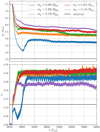 |
Fig. 17 Orbital elements of migrating planets in a circumbinary disc around the Kepler-413 system with different masses. Top panel: semi-major axis of the planet. Bottom panel eccentricity of the planet. The black lines show the observed values. The observed mass of Kepler-413b is mp = 0.211 Mjup. |
5 Discussion
Through 2Dhydrodynamical simulations, we first studied the structure of the circumbinary disc around five observed systems (Kepler-16, -34, -35, -38, and -413). After determining the structure of the inner disc (gap size and eccentricity as well as precession period of the gap), we inserted planets of various masses into our simulations and examined how they migrated through the disc andhow the presence of the planet changed the disc structure. In the following, we summarise the most important results of our simulations with and without planets.
5.1 Disc dynamics
Firstly, we looked at the structure of the inner gap created by the gravitational interaction between the binary and the disc. For simplicity, we restricted ourselves here to locally isothermal discs with a fixed aspect ratio (h = 0.05) and viscosity (α = 0.01) and studied different binary parameters. In agreement with previous studies (Miranda et al. 2017; Thun et al. 2017), we found that for all systems, the circumbinary discs became eccentric and showed a coherent slow prograde precession. Plotting the obtained precession period Tprec versus the obtained gap size agap, we confirmed the existence of two different branches for varying binary eccentricities, as shown in Fig. 3. As seen in the figure, the four systems, Kepler-16, 35, -38, and -413, fall exactly on the lower branch of the relation found in our first study (Thun et al. 2017). While Kepler-34 lays on the extreme end of the upper branch, due to the very large binary mass ratio and eccentricity of the system. To account for the different binary parameters, the y-axis has been rescaled according to the scaling of free particle orbits around binaries, Eq. (14).
In addition to these two known branches, we discovered a new behaviour for small binary eccentricities between ebin = 0.0 and ebin = 0.05. Starting from circular binaries, the precession period of the gap as well as the gap size increases up to ebin = 0.05. From there on, both quantities decrease again, as expected on the lower branch. At a critical ebin ≈ 0.18, the trend reverses again. A more detailed investigation of this additional new loop in the Tprec-agap diagram lies beyond the scope of this paper and is deferred to a future study.
In general, the five simulated systems behaved as expected and also the results from the two different codes used in this study, namely PLUTO and FARGO3D, produced matching results.
5.2 Evolution of embedded planets
After we had investigated the disc structure without the presence of a planet, we introduced planets to the simulations and studied how they migrated through the discs. The migration of planets and especially the final orbital parameters of the planets are important since it is assumed that planets in a P-type orbit around a binary form in the outer part of the disc, where the gravitational influence of the forming process due to the binary is negligible, and migrate inward to their final observed position.
Firstly, the disc without a planet was simulated until a quasi-steady state was reached, then we added the planet on a circular orbit for 2000 binary orbits so that the disc could adjust to the planet. After that initialisation period, the planet was allowed to freely move through the disc according to the disc torques acting on it. In the following, we summarise the main results using the example of Kepler-38.
Initial planet position: in a first simulation series, where we varied the initial planet position, we found that the final parking position of the planet does not depend on this initial planet location. In all cases, the planet migrates until it reaches the edge of the disc. At this point a strong positive corotation torque balances the negative Lindblad torque, responsible for inward migration, and the planet stops (Masset et al. 2006).
-
Variation of planet mass: when we varied the planet mass, we observed two different final configurations. In one state, the eccentricity of the planet is not excited and the planets remain on a nearly circular orbit around the binary. This low-eccentricity state applies for “massive” planets. These massive planets migrate smoothly through the disc until they reach their final position. During this migration process, they are able to alter the disc structure by shrinking and circularising the inner cavity of the disc. In contrast, the eccentricity of “lighter” planets becomes excited during their inward migration through the disc. Their migration path is not as smooth as in the massive planet case. An initial period of rapid inward migration is typically followed by a short and fast period of outward migration, that is again followed by a period of inward migration but with a much slower speed than in the first phase. During this migration through the disc, the orbit of the planets becomes fully aligned with the precessing inner gap of the disc and they end up in a state of apsidal corotation.
We were not able to find a sharp boundary between the massive and the light planets. The two different codes PLUTO and FARGO3D agreed well on the general migration behaviour of the planets (two eccentricity states) but showed small differences concerning the boundary between the two states of massive and light planets.
Variation of disc mass: a planet’s behaviour is not only determined by its mass but also the planet-to-disc mass ratio. In a simulation with a massive planet and a disc with reduced mass, we could observe that the massive planet behaves now like the light planets before, showing eccentricity excitation and orbital alignment. In other cases, we were able to switch the behaviour of a light planet to that of a massive one by decreasing the disc’s mass. Therefore, whether a planet in its final starting position shows an orbital alignment with the disc and an eccentric orbit or a more circular non-aligned orbit depends on the mass ratio between disc and planet.
Resonances: during our simulations, we quite often observed that planets were captured into a high-order resonance (11:1, 9:1, 8:1) with the binary. Planets which are trapped in a resonance do not migrate further to their observed location and their eccentricity is excited. We observed the capture into a resonance only for the “light” planet case during the second, slower inward migration phase.
The existence of two different eccentricity states was observed for the three systems Kepler-16, -35, and -38. For the systems Kepler-34 and -413, we could only observe the high eccentricity state for the light planet case with full orbital alignment between disc and planet. Even for planets with a mass around half a Jupiter mass or more, we were not able to trigger the massive planet case for these two systems. The reason for this behaviour could be the initial large and eccentric disc gaps in Kepler-34 and -413. Although the heavier planets were able to partly circularise the inner gap, they could never decrease the discs eccentricity below a value of 0.1. The two eccentricity states depend on the planet-to-disc mass ratio as well as on the binary parameters, since the latter determines the size and eccentricity of the disc’s gap for otherwise identical disc parameter like pressure and viscosity.
In this paper, we did not study the influence of the disc’s pressure and viscosity. In all simulations, we chose an aspect ratio of h = 0.05 and a viscosity of α = 0.01 to be consistent with our first paper, although an aspect ratio of h = 0.05 leads to rather high gas temperatures at the location of the planet. A comparison with a test simulation that also considered viscous heating and radiative cooling (for the same disc mass) suggests that an aspect ratio of h = 0.04 represents a more realistic gas temperature.
Test simulations of circumbinary discs around Kepler-38 with α = 0.001 and α = 0.05 show that in the case of low viscosity the observed planet with mass mp = 0.384 Mjup behaves accordingly to the light case, whereas in the case of high viscosity all three simulated planets with masses mp = {0.384, 0.300, 0.250} Mjup are able to dominate the disc. Since higher viscosity leads to a higher mass flow through the disc, the disc with α =0.05 is less massive than in our standard case; therefore all simulated planets are able to shrink and circularise the gap. In the case of α =0.001, the disc is more massive, meaning that even the planet with mass mp = 0.384 Mjup behaves like a light planet.
In general, we see both migration regimes if we vary the viscosity or the aspect ratio of the disc; only the final orbital parameters can change. This influence of the disc’s pressure and viscosity on the final orbital parameters of the planet needs to be examined infuture studies together with a more realistic equation of state rather than the isothermal one used in this study.
6 Summary
In all our simulations, the planet migration stopped at the inner boundary of the disc. However, the general observation in all five Kepler systems considered was that the planets stop their migration outside of the observed location; see Table 5. Two of the modelled systems (Kepler-16 and -38) ended up in the non-eccentric state where the final stopping point was about 30% larger than the observed locations, while the eccentricities were more or less comparable to the observed values. Kepler-35b reached an intermediate case where the final eccentricity was ep = 0.12 and a semi-major axis which was 30% larger than the observed one. Two systems (Kepler-34 and -413) ended up in the high eccentric, aligned state with a calculated final position about 1.5 times larger than the observed location and calculated eccentricities about 2–2.5 times larger than the observed ones. Although the final orbital elements did not match the observed ones very well, our simulations nevertheless did reproduce the fact that the systems with the highest gap eccentricity (Kepler-34 and -413) have the planets with the highest observed eccentricity among all systems considered in this study. We therefore suggest thatthe large observed planet eccentricities for these systems are caused by an eccentric circumbinary disc.
Nevertheless, because the calculated final position of the planets is too large in all cases, a mechanism is needed that is able to reduce the inner gap size of the disc to allow the planets to migrate further into the observed locations. One such mechanism could be disc self-gravity as described in Mutter et al. (2017b), although, according to the authors, only for very massive discs with masses ten times the minimum mass solar nebula or more, will the inner gap shrink further. Another way to reduce the disc’s gap size could be to change the disc parameters, such as pressure and viscosity. Increasing the temperature and/or the viscosity will produce smaller gaps. But as calculations in our first study (Thun et al. 2017) have shown, possibly unusually high pressures or viscosities may be needed to reduce the gap size substantially.
Furthermore, the impact that radiative effects have on the inner gap of the disc should be investigated. A good starting point will be simulations that include viscous heating and radiative cooling from the disc surface. Even more sophisticated simulations could also consider the radiative transport in the disc’s midplane and irradiation from the central binary. Finally, whether full 3D simulations will show different results remains to be seen. Considering the long timescales to be simulated, this is still numerically very challenging.
Acknowledgements
Daniel Thun was funded by grant KL 650/26 of the German Research Foundation (DFG). Most of the numerical simulations were performed on the bwForCluster BinAC. The authors acknowledge support by the High Performance and Cloud Computing Group at the Zentrum für Datenverarbeitung of the University of Tübingen, the state of Baden–Württemberg through bwHPC and the German Research Foundation (DFG) through grant no INST 37/935-1 FUGG. All plots in this paper were made with the Python library matplotlib (Hunter 2007).
Appendix A N-body solver for pluto
The N-bodysolver for PLUTO was developed by ourselves in the framework of this project and we briefly discuss some implementation details. In the discussion, we restrict ourselves to the 2D polar case. The PLUTO-code solves the hydrodynamic equations with the help of a finite-volume method which evolves volume averages in time. For the time evolution, we use the second-order Runge–Kutta method (RK2) provided by PLUTO. Given the hydrodynamical variables  at time tn, the positions
  and velocities
  of the N bodies (ℓ = 1, ...N) also at time tn, the whole system (hydrodynamical variables and N bodies) are advanced from time tn to tn+1 = tn + Δt using the following RK2 method:
 (A.1) (A.2)
For a definition of the “right-hand-side” operator  see Mignone et al. (2007). Here, U = (ϱ, ϱuR, ϱuφ) denotes the vector of conserved variables. The intermediate predictor state, U*, is given at time tn+1 which is important for the correct stepping of the N bodies. During the first RK2-substep (called A) we perform the following substeps:
- A1
Set boundaries.
- A2
Calculate disc feedback on each body ℓ (second term in Eq. (3))
![Mathematical equation: \begin{equation*} \begin{split} \vec{a}^n_{\mathrm{disc},\ell} \left(\vec{U}^n\right) = &\sum_{ij} \frac{G {\mathrm{\Sigma}}_{ij}^n \,\mathrm{d} V_{ij}} {\left[ (x_{c,ij}-x_{\ell}^n)^2+(y_{c,ij}-y_{\ell}^n)^2 +(\varepsilon h R_i)^2\right]^{3/2}}\\ &\quad \times\begin{pmatrix}x_{c,ij} - x_{\ell}^n\\ y_{c,ij} - y_{\ell}^n \end{pmatrix}, \end{split} \end{equation*}](/articles/aa/full_html/2018/08/aa32804-18/aa32804-18-eq31.png) (A.3)
(A.3)
where xc,ij = Ri cos(φj) and yc,ij = Ri sin(φj) denote the x- and y-coordinate of grid cell (i, j). The volume element dVij of this cell is given in polar coordinates by
 (A.4)
(A.4)
- A3
Calculate the acceleration (disc force and mutual gravitational attraction) on each of the N bodies (Eq. (3), first two terms)
![Mathematical equation: \begin{align*}\vec{a}_{\ell}^n =& \vec{a}^n_{\mathrm{grav},\ell} \left(\vec{x}^n_1,\dotsc,\vec{x}^n_N\right) +\vec{a}^n_{\mathrm{disc},\ell} \left(\vec{U}^n\right) \nonumber \\ \nonumber =& -\sum_{k \neq \ell}^{N} \frac{G M_k} {\left[ (x_{\ell}^n-x_k^n)^2 +(y_{\ell}^n-y_k^n)^2\right]^{3/2}} \begin{pmatrix}x_{\ell}^n-x_k^n \\ y_{\ell}^n-y_k^n \end{pmatrix} \\ &+\vec{a}^n_{\mathrm{disc},\ell} \left(\vec{U}^n \right.). \end{align*}](/articles/aa/full_html/2018/08/aa32804-18/aa32804-18-eq33.png) (A.5)
(A.5)
- A3
Calculate the indirect term, due to the acceleration of the centre of mass of the binary (Eq. (3), here 1 is the index of the primary and 2 is the index of the secondary).
 (A.6)
(A.6)
- A4
Hydro update
 . During this step we need to calculate the potential (Eq. (1)) at each cell location (i, j)
During the second RK2-substep (B) the following steps are necessary:
- B1
Set boundaries.
- B2
Advance bodies from xn to xn+1 using a fourth order Runge–Kutta integrator (RK4) using the acceleration from Eq. (A.5). In every substep of the RK4 integrator the mutual gravitational accelerations of the bodies are recalculated using the new substep positions (first term in Eq. (3)). For the disc feedback we use
 in every substep. After the N-body update we transform all quantities back to the centre of mass (let Xn+1 and Vn+1 denote the position and velocity of the centre of mass of the binary):

This simple shift accounts for the indirect term acom in Eq. (3).
- B2
Calculate acceleration of each body (Eq. (3)) using the updated body positions xn+1 and the updated hydro variables U*.
- B3
Calculate the indirect term, due to the acceleration of the centre of mass of the binary (Eq. (3)) using the accelerations of the binary from step B2.
- B4
Hydro update
 . During this step we need to calculate the potential (Eq. (1)) at each cell location.
Now all quantities (hydro and N-body positions) are at time tn+1 and a new RK2 cycle starts.
Appendix B Comparison with fargo3d
To test the implementation of our N-body solver for PLUTO we compared circumbinary disc simulations with an embedded planet for the Kepler-38 system with FARGO3D simulations (used in a 2D setup).
As briefly discussed in Sect. 2.3, FARGO3D uses an artificial viscosity (AV) to smooth out shocks over various cells. The strength of the artificial viscosity is controlled by the constant Cav. This constant is basically the number of cells over which the shock is smoothed. To study the impact of AV on the disc dynamics, we varied the constant Cav leaving the physical setup unchanged Fig. B.1 shows that the strength of the AV can change the simulation outcome significantly. Shown is the time evolution of the inner disc eccentricity for the Kepler-38 system. The eccentricity obtained with the standard artificial viscosity constant of FARGO3D (Cav = 1.41, orange curve) does not reproduce the PLUTO result (blue curve). To obtain a better agreement between the codes, we had to reduce the artificial viscosity used in FARGO3D to Cav = 0.5. Using these adjustments, the new FARGO3D results (green curve in Fig. B.1) and the PLUTO agree very well indeed. Simulations with no artificial viscosity are not stable at all (red curve in Fig. B.1).
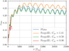 |
Fig. B.1 Time evolution of the disc eccentricity for the Kepler-38 system. The blue curve shows a PLUTO simulation, while all other curves show results from FARGO3D simulations, where the strength of the artificial viscosity was varied. |
For the rest of this section, we compare PLUTO and FARGO3D simulations of a circumbinary disc around Kepler-38 with an embedded planet. Figure B.2 shows the semi-major axis (top row) and the eccentricity time evolution (bottom row) of five planets with different masses from mp = 0.150 Mjup to mp = 0.384 Mjup. The left column shows PLUTO results whereas the right column shows FARGO3D results. The codes agree very well for the mp = 0.384 Mjup case (blue curve in Fig B.2). In both simulations the planet smoothly migrates inward until it reaches a final position slightly below 4 abin. In the FARGO3D simulations the planet migrates faster and a little bit more inward. Additionally, in both simulations the eccentricity of the massive planet stays below 0.05.
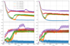 |
Fig. B.2 Orbital elements of planets with different mass. Top panel: semi-major axis of the planets. Bottom panel: eccentricity. Left column: PLUTO simulations. Right column: FARGO3D simulations. |
The codes produce also in the mp = 0.150 Mjup case the same results. This lighter planet does not migrate as far inward as the massive planet discussed earlier. It reaches its final parking position at roughly 5 abin, but its eccentricity is increased to a value between 0.2 and 0.25. In both simulations the planet is captured in a 11:1 resonance with the binary. The only difference here is that in the PLUTO simulation the planet is kicked out of this resonance while in the FARGO3D simulations the planet remains in resonance with the binary. A more detailed analysis of the resonance can be found in Sect. 4.1.2.
For the planets with masses mp = 0.250 Mjup and mp = 0.300 Mjup, the two codes produce the same overall behaviour but deviate in the details. As discussed in Sect. 4.1.2, these planets migrate first inward, then they reverse their migration direction and undergo a period of fast outward migration. After that they start to migrate inward again but on a much longer timescale than during the first inward migration period. This behaviour is observed with both codes. In the FARGO3D simulations the planets start their outward migration period in both cases a bit earlier than in the PLUTO simulations. A reason why in the PLUTO simulations the planets’ outward migration period starts at different times could be the fact that the mp = 0.300 Mjup planet is briefly captured in a 8:1 resonance with the binary between t = 27 000 Tbin and t = 30 000 Tbin. But besides these differences the codes produce the results in good agreement for the final orbital parameters of the planets. A final position around 4.5 abin and an increased eccentricity of around 0.20.
For the case mp = 0.200 Mjup, the codes differ in the final orbital elements of the planet. In the PLUTO simulations, this planet ends up with orbital parameters like the light planet with mass mp = 0.150 Mjup, whereas in the FARGO3D simulations the planet’s final orbital parameter are similar to the intermediate planets with mp = 0.250 Mjup and mp = 0.200 Mjup. As discussed in the main part of this paper, we observe a different migration behaviour and different final orbital elements for light and massive planets. For very massive and very light planets the codes produce consistent and matching results. However, the exact point (in mass) at which the transition between massive and lighter planets occurs depends somewhat on the code used. Whether intermediate mass planets land on the massive or light branch depends on the code, but the absolute difference in mass is not very large. This was not only observed for the Kepler-38 system but also for Kepler-16 and -35.
For example, a FARGO3D simulation of Kepler-35 with a planet of mass mp = 0.550 Mjup shows the same results as the PLUTO simulation. But results of a FARGO3D simulation with planet mass mp = 0.500 Mjup shows the behaviour of a light planet (eccentricity excitation, orbital alignment), whereas in PLUTO simulations the mp = 0.500 Mjup planet is on the massive branch (see Sect. 4.4).
For the Kepler-34 and -413 systems, we only observed one state with both codes. In both codes, the large and highly eccentric inner gap always dominated the planet.
Finally, we comment on the code performance on this problem. In Table B.1, we compare the average CPU-time per time step in seconds for PLUTO and FARGO3D for simulations of a disc around Kepler-38 with and without an embedded planet. The simulations that used a numerical resolution of 684 × 584 grid cells were carried out on one or two Nvidia Titan X GPUs. As seen, the two codes show a relatively similar performance in spite of the different numerical methods used. For both codes, the runs on two GPUs are about 1.6 times faster that on a single GPU.
Average CPU-time per time step in seconds for PLUTO and FARGO3D test simulations (using 684 × 584 grid cells) with and without planet.
References
- Artymowicz, P., & Lubow, S. H. 1994, ApJ, 421, 651 [NASA ADS] [CrossRef] [Google Scholar]
- Benítez-Llambay, P., & Masset, F. S. 2016, ApJS, 223, 11 [NASA ADS] [CrossRef] [Google Scholar]
- Crida, A., Morbidelli, A., & Masset, F. 2006, Icarus, 181, 587 [Google Scholar]
- de Val-Borro, M., Edgar, R. G., Artymowicz, P., et al. 2006, MNRAS, 370, 529 [NASA ADS] [CrossRef] [Google Scholar]
- Doyle, L. R., Carter, J. A., Fabrycky, D. C., et al. 2011, Science, 333, 1602 [NASA ADS] [CrossRef] [MathSciNet] [PubMed] [Google Scholar]
- Dvorak, R. 1986, A&A, 167, 379 [NASA ADS] [Google Scholar]
- Günther, R., & Kley, W. 2002, A&A, 387, 550 [NASA ADS] [CrossRef] [EDP Sciences] [MathSciNet] [Google Scholar]
- Holman, M. J., & Wiegert, P. A. 1999, AJ, 117, 621 [NASA ADS] [CrossRef] [Google Scholar]
- Hunter, J. D. 2007, Comput. Sci. Eng., 9, 90 [Google Scholar]
- Kley, W., & Haghighipour, N. 2014, A&A, 564, A72 [NASA ADS] [CrossRef] [EDP Sciences] [Google Scholar]
- Kley, W., & Haghighipour, N. 2015, A&A, 581, A20 [NASA ADS] [CrossRef] [EDP Sciences] [Google Scholar]
- Kostov, V. B., McCullough, P. R., Carter, J. A., et al. 2014, ApJ, 784, 14 [NASA ADS] [CrossRef] [Google Scholar]
- Kostov, V. B., Orosz, J. A., Welsh, W. F., et al. 2016, ApJ, 827, 86 [NASA ADS] [CrossRef] [Google Scholar]
- Lin, D. N. C., & Papaloizou, J. 1986, ApJ, 309, 846 [NASA ADS] [CrossRef] [Google Scholar]
- Lines, S., Leinhardt, Z. M., Baruteau, C., Paardekooper, S.-J., & Carter, P. J. 2015, A&A, 582, A5 [Google Scholar]
- Marzari, F., Thébault, P., & Scholl, H. 2008, ApJ, 681, 1599 [NASA ADS] [CrossRef] [Google Scholar]
- Masset, F. S., Morbidelli, A., Crida, A., & Ferreira, J. 2006, ApJ, 642, 478 [NASA ADS] [CrossRef] [Google Scholar]
- Meschiari, S. 2012, ApJ, 761, L7 [NASA ADS] [CrossRef] [Google Scholar]
- Mignone, A., Bodo, G., Massaglia, S., et al. 2007, ApJS, 170, 228 [Google Scholar]
- Miranda, R., Muñoz, D. J., & Lai, D. 2017, MNRAS, 466, 1170 [NASA ADS] [CrossRef] [Google Scholar]
- Müller, T. W. A., Kley, W., & Meru, F. 2012, A&A, 541, A123 [NASA ADS] [CrossRef] [EDP Sciences] [Google Scholar]
- Mutter, M. M., Pierens, A., & Nelson, R. P. 2017a, MNRAS, 465, 4735 [NASA ADS] [CrossRef] [Google Scholar]
- Mutter, M. M., Pierens, A., & Nelson, R. P. 2017b, MNRAS, 469, 4504 [NASA ADS] [CrossRef] [Google Scholar]
- Nelson, R. P., & Papaloizou, J. C. B. 2002, MNRAS, 333, L26 [NASA ADS] [CrossRef] [Google Scholar]
- Nelson, R. P., Papaloizou, J. C. B., Masset, F., & Kley, W. 2000, MNRAS, 318, 18 [NASA ADS] [CrossRef] [Google Scholar]
- Orosz, J. A., Welsh, W. F., Carter, J. A., et al. 2012a, ApJ, 758, 87 [NASA ADS] [CrossRef] [Google Scholar]
- Orosz, J. A., Welsh, W. F., Carter, J. A., et al. 2012b, Science, 337, 1511 [NASA ADS] [CrossRef] [PubMed] [Google Scholar]
- Paardekooper, S.-J., Leinhardt, Z. M., Thébault, P., & Baruteau, C. 2012, ApJ, 754, L16 [NASA ADS] [CrossRef] [Google Scholar]
- Pierens, A., & Nelson, R. P. 2007, A&A, 472, 993 [NASA ADS] [CrossRef] [EDP Sciences] [Google Scholar]
- Pierens, A., & Nelson, R. P. 2008, A&A, 483, 633 [NASA ADS] [CrossRef] [EDP Sciences] [Google Scholar]
- Pierens, A., & Nelson, R. P. 2013, A&A, 556, A134 [NASA ADS] [CrossRef] [EDP Sciences] [Google Scholar]
- Scholl, H., Marzari, F., & Thébault, P. 2007, MNRAS, 380, 1119 [NASA ADS] [CrossRef] [Google Scholar]
- Schwamb, M. E., Orosz, J. A., Carter, J. A., et al. 2013, ApJ, 768, 127 [NASA ADS] [CrossRef] [Google Scholar]
- Shakura, N. I., & Sunyaev, R. A. 1973, A&A, 24, 337 [NASA ADS] [Google Scholar]
- Silsbee, K., & Rafikov, R. R. 2015, ApJ, 808, 58 [NASA ADS] [CrossRef] [Google Scholar]
- Stone, J. M., & Norman, M. L. 1992, ApJS, 80, 753 [Google Scholar]
- Tanaka, H., Takeuchi, T., & Ward, W. R. 2002, ApJ, 565, 1257 [NASA ADS] [CrossRef] [Google Scholar]
- Thun, D., Kley, W., & Picogna, G. 2017, A&A, 604, A102 [NASA ADS] [CrossRef] [EDP Sciences] [Google Scholar]
- Ward, W. R. 1997, Icarus, 126, 261 [NASA ADS] [CrossRef] [Google Scholar]
- Welsh, W. F., Orosz, J. A., Carter, J. A., et al. 2012, Nature, 481, 475 [NASA ADS] [CrossRef] [PubMed] [Google Scholar]
- Welsh, W. F., Orosz, J. A., Short, D. R., et al. 2015, ApJ, 809, 26 [NASA ADS] [CrossRef] [Google Scholar]
Kepler-16 (Doyle et al. 2011), Kepler-34 and -35 (Welsh et al. 2012), Kepler-38 (Orosz et al. 2012a), Kepler-47 (Orosz et al. 2012b), Kepler-64 (Schwamb et al. 2013), Kepler-413 (Kostov et al. 2014), Kepler-453 (Welsh et al. 2015), and Kepler-1647 (Kostov et al. 2016).
We use the following notation: R is the 2D position vector in the x − y-plane, R = RêR.
In all simulations, we use the following code units: R0 =abin, M0 = Mbin,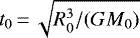 and
and , with the gravitational constant G.
We use a modified version of PLUTO 4.2 which runs on GPUs and is also capable of solving a N-body system.
All Tables
Planet mass mp, disc mass Mdisc and the ratio q = mp∕Mdisc for models using different disc masses.
Final orbital parameters of the embedded planets using the observed mp for the five systems investigated, calculated using the PLUTO simulations.
Average CPU-time per time step in seconds for PLUTO and FARGO3D test simulations (using 684 × 584 grid cells) with and without planet.
All Figures
|
Fig. 1 Azimuthally averaged surface density at various times for the Kepler-38 system calculated with PLUTO. The blue curve shows the initial density distribution. The black vertical line marks the 1 abin location where the density would reach the reference density if we had not imposed an initial gap (blue curve). The dashed horizontal lines mark the reference density (in black) and the density floor (in red). |
| In the text | |
|
Fig. 2 The precession period, semi-major axis, and eccentricity of the disc gap vs. time, for our five different systems. Disc models on the left are calculated with PLUTO and disc models on the right are calculated with FARGO3D. The precession period, Tprec, in the first row is given in terms of the corresponding period number. The horizontal lines indicate the time average starting from 6000 binary orbits, roughly the time when the discs reached a quasi-steady state. See the text for an explanation of the meaning of the + and × signs in the first row. |
| In the text | |
|
Fig. 3 Precession period of the inner gap, scaled by the factor |
| In the text | |
|
Fig. 4 Gap eccentricity plotted against the semi-major axis of the gap. Different bullets correspond to numerical results for different binary eccentricities whereas different colours stand for different binary mass ratios. The five different Kepler systems considered in this paper are marked by the black stars. |
| In the text | |
|
Fig. 5 Azimuthally averaged density profiles after 10 000 binary orbits for the five different Kepler systems. The dots mark the initial planet position. |
| In the text | |
|
Fig. 6 Time evolution of the semi-major axis of a mp = 0.384 Mjup planet with different initial positions in a circumbinary disc around the Kepler-38 system. The black line shows the observed position of the planet. |
| In the text | |
|
Fig. 7 Azimuthally averaged density profiles for the Kepler-38 disc with embedded planets after 12 000 binary orbits. The planets were held on a fixed orbit (ap = 6.0 abin) for 2000 binary orbits. |
| In the text | |
|
Fig. 8 Orbital elements of migrating planets in a circumbinary disc around the Kepler-38 system with different masses. Top panel: semi-major axis of the planet. Bottom panel: eccentricity of the planet. The black lines show the observed values, for the eccentricity only an upper limit is known. The upper mass limit for Kepler-38b is mp = 0.384 Mjup. |
| In the text | |
|
Fig. 9 Three out of eleven resonant angles for the mp = 0.150 Mjup case. While the resonant angles Φ1 and Φ3 cover the fullrange from 0 to 2π the resonant angle Φ2 librates around zero during the resonant phase of the planet (from t = 34 000 Tbin to t = 45 000 Tbin). The resonant angles Φ3 to Φ11 also cover the full range from 0 to 2π but are not shown for clarity. |
| In the text | |
|
Fig. 10 Structure of the inner disc for the Kepler-38 system. The surface density is colour-coded, since the absolute density values are not important for the disc structure we omit the density scale for clarity (brighter colours mean higher surface densities). The top-left panel shows the circumbinary disc after 10 000 binary orbits before the planet is inserted. The remaining three panels show the disc structure with an embedded planet of varying mass after 76 500 binary orbits. The binary components and the planets are marked with black dots. The direction of pericentre of the secondary (green), the planet (blue), and the disc (orange) are marked by the arrows. Additional fitted ellipses to the central cavity are plotted in dashed white lines and the actual orbit of the planet is shown as dashed blue line. Using the fitted ellipses, the size and eccentricity of the disc gap, shown in the upper left edge of each panel, are calculated at the same time. As we saw in Fig. 2 these quantities show small variations in time around some average value. |
| In the text | |
|
Fig. 11 Time evolution of the inner disc eccentricity for Kepler-38. Planets of different mass were introduced into the simulations at 10 000 binary orbits on circular orbits and allowed to migrate through the disc after 12 000 binary orbits. |
| In the text | |
|
Fig. 12 Time evolution of the pericentres of a planet with mass mp = 0.250 Mjup (blue) and the disc (orange) for Kepler-38. Until t = 12 000 Tbin the planet ison a fixed circular orbit and therefore the pericentre is not well defined. After switching on the back-reaction onto the planet, its orbit soon becomes aligned with the inner precessing cavity of the disc. |
| In the text | |
|
Fig. 13 Time evolution of semi-major axis (top) and eccentricity (bottom) of planets with different mass in discs of different mass, for the Kepler-38 system. |
| In the text | |
|
Fig. 14 Orbital elements of migrating planets in a circumbinary disc around the Kepler-16 system with different masses. Top panel: semi-major axis of the planet. Bottom panel: eccentricity of the planet. The black lines show the observed values. The observed mass of Kepler-16b is mp = 0.333 Mjup. |
| In the text | |
|
Fig. 15 Orbital elements of migrating planets in a circumbinary disc around the Kepler-34 system with different masses. Top panel: semi-major axis of the planet. Bottom panel: eccentricity of the planet. The black lines show the observed values. The observed mass of Kepler-34b is mp = 0.220 Mjup. |
| In the text | |
|
Fig. 16 Orbital elements of migrating planets in a circumbinary disc around the Kepler-35 system with different masses. Top panel: semi-major axis of the planet. Bottom panel: eccentricity of the planet. The black lines show the observed values. The observed mass of Kepler-35b is mp = 0.127 Mjup. |
| In the text | |
|
Fig. 17 Orbital elements of migrating planets in a circumbinary disc around the Kepler-413 system with different masses. Top panel: semi-major axis of the planet. Bottom panel eccentricity of the planet. The black lines show the observed values. The observed mass of Kepler-413b is mp = 0.211 Mjup. |
| In the text | |
|
Fig. B.1 Time evolution of the disc eccentricity for the Kepler-38 system. The blue curve shows a PLUTO simulation, while all other curves show results from FARGO3D simulations, where the strength of the artificial viscosity was varied. |
| In the text | |
|
Fig. B.2 Orbital elements of planets with different mass. Top panel: semi-major axis of the planets. Bottom panel: eccentricity. Left column: PLUTO simulations. Right column: FARGO3D simulations. |
| In the text | |
Current usage metrics show cumulative count of Article Views (full-text article views including HTML views, PDF and ePub downloads, according to the available data) and Abstracts Views on Vision4Press platform.
Data correspond to usage on the plateform after 2015. The current usage metrics is available 48-96 hours after online publication and is updated daily on week days.
Initial download of the metrics may take a while.