| Issue |
A&A
Volume 616, August 2018
|
|
|---|---|---|
| Article Number | A67 | |
| Number of page(s) | 19 | |
| Section | Interstellar and circumstellar matter | |
| DOI | https://doi.org/10.1051/0004-6361/201732553 | |
| Published online | 17 August 2018 | |
Complex cyanides as chemical clocks in hot cores
1
Kapteyn Astronomical Institute, University of Groningen,
Groningen,
The Netherlands
e-mail: This email address is being protected from spambots. You need JavaScript enabled to view it.
2
SRON,
Groningen,
The Netherlands
e-mail: This email address is being protected from spambots. You need JavaScript enabled to view it.
3
School of Physics and Astronomy, University of Leeds,
Leeds
LS2 9JT,
UK
Received:
26
December
2017
Accepted:
21
March
2018
Abstract
Context. In the high-mass star-forming region G35.20−0.74N, small scale (~800 AU) chemical segregation has been observed in which complex organic molecules containing the CN group are located in a small location (toward continuum peak B3) within an apparently coherently rotating structure.
Aims. We aim to determine the physical origin of the large abundance difference (~4 orders of magnitude) in complex cyanides within G35.20−0.74 B, and we explore variations in age, gas/dust temperature, and gas density.
Methods. We performed gas-grain astrochemical modeling experiments with exponentially increasing (coupled) gas and dust temperature rising from 10 to 500 K at constant H2 densities of 107 cm−3, 108 cm−3, and 109 cm−3. We tested the effect of varying the initial ice composition, cosmic-ray ionization rate (1.3 × 10⁻¹⁷ s−1, 1 × 10⁻¹⁶ s−1, and 6 × 10⁻¹⁶ s−1), warm-up time (over 50, 200, and 1000 kyr), and initial (10, 15, and 25 K) and final temperatures (300 and 500 K).
Results. Varying the initial ice compositions within the observed and expected ranges does not noticeably affect the modeled abundances indicating that the chemical make-up of hot cores is determined in the warm-up stage. Complex cyanides vinyl and ethyl cyanide (CH2CHCN and C2H5CN, respectively) cannot be produced in abundances (vs. H2) greater than 5 ×10⁻¹⁰ for CH2CHCN and 2 ×10⁻¹⁰ for C2H5CN with a fast warm-up time (52 kyr), while the lower limit for the observed abundance of C2H5CN toward source B3 is 3.4 ×10⁻¹⁰. Complex cyanide abundances are reduced at higher initial temperatures and increased at higher cosmic-ray ionization rates. Reaction-diffusion competition is necessary to reproduce observed abundances of oxygen-bearing species in our model.
Conclusions. Within the context of this model, reproducing the observed abundances toward G35.20−0.74 Core B3 requires a fast warm-up at a high cosmic-ray ionization rate (~1 × 10⁻¹⁶ s−1) at a high gas density (>109 cm−3). The abundances observed at the other positions in G35.20-0.74N also require a fast warm-up but allow lower gas densities (~108 cm−3) and cosmic-ray ionization rates (~1 × 10⁻¹⁷ s−1). In general, we find that the abundance of ethyl cyanide in particular is maximized in models with a low initial temperature, a high cosmic-ray ionization rate, a long warm-up time (>200 kyr), and a lower gas density (tested down to 107 cm−3). G35.20−0.74 source B3 only needs to be ~2000 years older than B1/B2 for the observed chemical difference to be present, which maintains the possibility that G35.20−0.74 B contains a Keplerian disk.
Key words: stars: massive / astrochemistry / ISM: individual objects: G35.20−0.74N / ISM: molecules
© ESO 2018
1 Introduction
In high-mass star formation, the hot molecular core (HMC) stage is marked by high abundances of complex organic molecules (COMs), molecular species containing at least six atoms including carbon and hydrogen (Herbst & van Dishoeck 2009), and emitting from a warm (100–500 K), dense (nH > 107 cm−3), and compact (<0.05 pc) region. The physical nature of this type of region, whether a disk, an outflow cavity, or an envelope, is currently unknown. The COMs seen in hot cores are expected to be abundantly produced in the ice mantles hosted on dust grains around the forming star and released into the gas phase upon warming. Also, COMs can be produced through endothermic reactions in warm gas. The HMC stage is not expected to last more than 105 years, as COMs are dissociated in the expanding HII region around a young high-mass star. As a short-lived stage with specific physical parameters, the HMC is an ideal source for studying the process of high-mass star formation and by tracing the distribution of specific molecular species, we can learn more about the physical and chemical structure of these young objects.
Chemical segregation has been observed in several different star-forming regions on scales from 1000 to 8000 AU, most famously in Orion KL where Blake et al. (1987) observed that the hot core has a much higher abundance of N-bearing species than the compact ridge and surrounding sources. To explain this, Caselli et al. (1993) modeled shells of gas collapsing toward the nearby object IRc2, which are halted and heated up showing different chemical compositions (see Feng et al. 2015 and Crockett et al. 2015 for recent work on Orion KL). A difference in chemical composition has also been seen between W3(OH) and W3(H2O) (Wyrowski et al. 1999) where the latter is a strong N-bearing source with various complex organics, but the former only contains a handful of O-bearing species. AFGL2591 VLA 3 is another source (Jiménez-Serra et al. 2012) where such chemical segregation has been observed on a scale of a few thousand AU, which was explained using models of concentric shells with different temperatures and amounts of extinction.
This paper follows our previous study (Allen et al. 2017) of G35.20-0.74N (G35.20), a high-mass star-forming region containing several high-mass protostars at a distance of 2.19 kpc with a bolometric luminosity of 3.0 ×10⁴ L⊙ (Sánchez-Monge et al. 2014). G35.20 was shown to be a strong Keplerian disk candidate based on position-velocity diagrams for several species and the fit of the velocity field to a Keplerian disk model (Sánchez-Monge et al. 2013). In this source, we observed a segregation in Core B between complex N-bearing species, especially cyanides (those containing the CN group), and other COMs on a scale of less than 1000 AU within an apparently coherent source presenting a potential signature of Keplerian rotation. Within Core B (shown in Fig. 1) there is a higher abundance (generally 1–2 orders of magnitude) of almost all observed species to the southeast (at continuum peak B3), and additionally, the nitrogen-bearing species abundance drops quickly when proceeding to the northwest (to continuum peaks B1 and B2 about 1000 and 2000 AU from source B3, respectively) where most complex N-bearing species (especially those with the CN group) are no longer detected. This is especially prominent in ethyl- and vinyl cyanide (C2 H5CN and CH2CHCN) and in vibrationally excited states and isotopologs of methyl cyanide (CH3 CN) and cyanoacetylene (HC3N). We also model the observed abundances from Core A for comparison, as it is not part of the potential Core B disk system, but has a similar chemical composition to source B3 with high abundances of cyanides and oxygen-bearing species.
We expect G35.20 source B3 to be a high-mass source as a high kinetic temperature is observed toward peak B3 (~300 K) compared topeak B1 and peak B2 (160 and 120 K, respectively). Alongside this high temperature, the deuterium fraction is very high toward source B3 (13% for CH3CN) implying that it has only recently heated up, releasing deuterium enriched ices into the gas phase. There is also a cluster of OH masers toward peak B3 (Hutawarakorn & Cohen 1999). At the outer radius of this disk candidate, the rotation period is between 9700 and 11 100 years, which is fast enough that such a difference in chemistry should not be present because of the mixing of gas. In this work, we use chemical modeling to investigate a cause for chemical segregation between complex cyanides and other species related to age, temperature, warm-up time, or gas density.
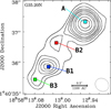 |
Fig. 1 870 μm continuum emission from Cycle 0 ALMA observations of G35.20. The continuum peaks are labeled in order of intensity (i.e., peak B1 has the highest and peak B3 the lowest continuum intensity). Contour levels are 0.03, 0.042, 0.055, 0.067, 0.08, 0.10, 0.13, 0.18, and 0.23 Jy beam−1 (σ = 1.8 mJy beam−1). The pixel-sized colored squares denote each of the spectral extraction points (from Allen et al. 2017). |
2 Chemical model
2.1 Model setup
We used a large gas-grain chemical network (668 species, over 8000 reactions) in which the gas-phase reactions are from the UMIST Database for Astrochemistry (McElroy et al. 2013) known as Rate121, and the grain-surface and gas-grain interactions are extracted from the Ohio State University (OSU) network (detailed description in Walsh et al. 2014). Our network includes the following reaction types: two-body gas-phase reactions, direct cosmic-ray ionization, cosmic-ray-induced photoreactions, photoreactions, cation–grain recombination, adsorption onto grains, thermal desorption, photodesorption, grain-surface cosmic-ray-induced photoreactions, grain-surface photoreactions, two-body grain-surface reactions, and reactive desorption.
In this model, the thermal desorption rate depends on the binding energy of the species (Ebind, A) and the number density of that species on the grain-surface (ns(A)). If there are less than two monolayers, then the following first order rate is used: fthermal,A = kevap,Ans(A) (Cuppen et al. 2017), where kevap,A = ν exp−Ebind,A/kT and ν is the characteristic attempt frequency. Once there are more than two monolayers, then the following zeroth-order approximation: fthermal,A =kevap,ANactχANsσgngrain, where Nact is the number of active monolayers, χA is the fractional abundance of species A, and Nsσgngrain is the number of available surface sites per unit volume. Further details about this chemical code can be found in Drozdovskaya et al. (2014) and Walsh et al. (2014, 2015). Reaction–diffusion competition is included.
The model considers a single embedded (AV = 10) point sourceat a constant gas density that is warming up over time. The relatively high extinction means that the only source of ionization and photodissociation in the model is cosmic rays. A low cosmic-ray ionization rate of 1.3 ×10⁻¹⁷ s−1 was used in the fiducial model. Higher cosmic-ray ionization rates are explored in test cases (Sects. 3.2–3.6).
2.2 Initial conditions
We start a warm-up phase at the end of a theoretical collapse phase that results in a constant H2 density of n= 107, 108, or 109 cm−3 with enhanced ice abundances of several species (see Table 1). The gas density of Core B is expected to be 107 –108 cm−3 and Core A is expected to have a density of 109 cm−3 from Sánchez-Monge et al. (2014). The warm-up phases start with the initial conditions (IC) outlined in Table 1 and the (coupled) gas and dust temperature increases from 10 to 500 K over 52 (fast), 203 (medium), or 1000 (slow) kyr according to the equation T(t) = 10 + κt2 as based upon the methods in Viti et al. (2004), Garrod & Herbst (2006), and Garrod et al. (2008). The values of κ used in this workto warm from 10 to 500 K in the prescribed times for the fast, medium, and slow warm-ups are 1.96× 10⁻²², 1.2 × 10⁻²³, and 4.9 × 10⁻²⁵ K s−2, respectively.
The initial ice abundances for IC 2, 4, and 5 are from ice observations carried out by Gibb et al. (2004) of three high-mass star-forming regions, i.e., AFGL 2136, W33A, and NGC 7538 IRS9, respectively.Initial conditions (IC) 1 and 3 are based on a lower limit of the water abundance of 10−5 vs. H2 and an upper limit of water abundance of 10−4 vs. H2 as suggested in van Dishoeck (2004). Other molecular abundances in IC 1 and 3 are then percentages of 5% (for NH3, CH3OH, and CH4 ice) or 10% (for CO, CO2, HCOOH, and H2CO ice) of water. The atomic gas abundances in our model are the result of subtracting the atoms that have gone into molecules from the typical gas abundances found in the pristine model input. Our approach differs from Garrod et al. (2008) in that their model includes a phase of initial collapse from diffuse cloud to dense core, thereby building up their ices in a model-dependent manner. Our full gas and ice initial conditions are detailed in Appendix A. While we did not include molecular gas in our initial abundances, the chemistry quickly converts the free atoms into stable molecules (Fig. 2). These gas-phase abundances are within an order of magnitude of reported abundances in starless and prestellar cores (Ruoskanen et al. 2011; Koumpia et al. 2016; Vastel et al. 2016).
Initial ice composition vs. H2O ice.
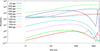 |
Fig. 2 Abundances of simple species over time for a fast warm-up with a gas density of 107 cm−3. Dashed lines show ice abundances and solid lines show gas abundances. |
2.3 Modeling approach
First, we tested the fiducial model (Sect. 3.1): three different densities (based on the expected densities of our observed sources) at three different warm-up speeds based on expected gas warming speed around low-, intermediate-, and high-mass stars (discussed in Sect. 4.3) for the five initial conditions outlined above (Sect. 2.2). After the basic test, we tested models that each changed one feature of the fiducial model for a fast warm-up (as expected for a high-mass source). These were, excluding reaction–diffusion competition (Sect. 3.2), changing the initial temperature to 15 or 25 K (Sect. 3.3), running time at a high temperature (300 K) after the warm-up period (Sect. 3.4), adding HCN to the initial ice (Sect. 3.5), and raising the cosmic-ray ionization rate to 1 × 10⁻¹⁶ s−1 and 6 × 10⁻¹⁶ s−1 (Sect. 3.6). Modeled abundances for each test were compared to the observed abundances from Allen et al. (2017) shown in Table 2 and their associated upper and lower limits to constrain the time period during which all abundances could be reproduced by the model.
Abundances vs. H2 across G35.20 from Allen et al. (2017).
3 Results
We aim to constrain the time periods during which the models reasonably reproduce the observed abundances within observed error limits (detailed in Table 2) of the following molecules: cyanides (CH3CN, CH2CHCN, C2 H5CN), cyanoacetylene (HC3N), methanol (CH3OH), methyl formate (CH3OCHO), acetaldehyde (CH3CHO), and ethanol (C2 H5OH). For a time period to be an acceptable fit, its duration must be less than half a disk rotation period (<5 kyr). The focus species include all of the cyanides observed in G35.20 and most of the complex organic oxygen-bearing species. The abundances in Table 2 were determined using detailed modeling of ALMA observations of spectral lines from the four continuum points in Fig. 1 (Allen et al. 2017) using the software XCLASS (Möller et al. 2017), assuming local thermal equilibrium (LTE). The key result from this analysis was that continuum peak B3 showed higher abundances of almost all modeled species, but especially of those containing the CN group. Two in particular, vinyl and ethyl cyanide (CH2CHCN, C2 H5CN), were not detected at continuum peaks B1 and B2, giving an upper limit to their abundances of 1 × 10⁻¹³ with respectto H2. Upper and lower limits for the XCLASS modeling results can be found in Appendix B.
We find little variation among the different starting conditions (see Fig. 3), so in the following analysis we use the initial ice composition of IC5 as NGC 7538 IRS9 has a similar bolometric luminosity and distance to G35.20 (4 × 10⁴ L⊙ and 2.7 kpcfor NGC 7538 IRS9 vs. 3 × 10⁴ L⊙ and 2.2 kpc for G35.20).
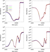 |
Fig. 3 Fractional abundance vs. H2 for one species with different initial conditions (ICs 1-5) for a gas density of 107 cm−3 and a fast warm-up time of 50 kyr. Results are similar for other warm-up times and densities. |
3.1 Fiducial model
In our fiducial model, we begin with gas and dust at 10 K and the initial ice and gas conditions of IC5, then warm the gas and dust at fast, medium, and slow speeds (detailed in Sect. 2.1) to 500 K at a constant gas density. All of the tests in the following subsections begin with the conditions of this fiducial model varying one parameter. Time ranges and corresponding gas temperature ranges for all fits are summarized in Table 3.
Fast warm-up models can reproduce all of the abundances observed for peaks B1/B2 and the C2 H5CN abundance can be reproduced in core A for densities of n =107 and 108 cm−3. The model C2 H5CN abundance at peak B3 cannot be reproduced by the fiducial model, although at a density of 107 cm−3 it is 1.4 × 10⁻¹⁰ lower (50%) than the minimum observed abundance (see Fig. 4). This difference is significantly larger than the tolerance for the model (10−13) and is therefore not a fit. A summary of the time periods where the observed abundances of HC3N, CH3CN, CH2CHCN, C2 H5CN, CH3OCHO, and C2 H5OH are reproduced in a fast warm-up for all sources and gas densities is shown in Fig. 5.
Medium-speed warm-up models can reproduce the C2 H5CN abundance observed in source B3 at late times (after 97 kyr). The time period required to reproduce all observed abundances is >13 kyr, which is longer than a disk rotation period. Abundances in source B1/B2 can be reproduced in a medium warm-up in ~5.5 kyr. See Appendix D for tables detailing the times at which observed abundances are replicated by the fiducial model and further plots of abundance over time.
Slow warm-up models for all three densities can reproduce all of the observed abundances.The time periods needed to reproduce the observed abundances are shorter for n =108 and 109 cm−3, although still very long (>40 kyr). For peaks B1/B2 the shortest time range is 40 kyr at n =109 cm−3 (temperature range 96–113 K). The shortest time range for peak B3 is 65 kyr, corresponding to a temperature range of 102–132 K at n =109 cm−3. These time ranges are not reasonable, as the gas in the disk would have made several revolutions during such a long period.
The fiducial model fits peaks B1/B2 and core A very well using a fast warm-up. Abundances toward peaks B1/B2 can even be reproduced within a time period of 1.3 kyr at a gas density of 108 cm−3. Core A requires a longer time period of 6.4 kyr, but is still well fit at a gas density of 108 cm−3 with a fast warm-up. The best fit models for B1/B2 and A are shown in Fig. 6. The abundances of C2 H5CN toward peak B3 cannot be reproduced using a fast warm-up, but the shortest time period (13 kyr) that reproduces all abundances is using a medium warm-up at a gas density of 107 cm−3. This is too long kinematically (the disk rotational period is ~10 kyr), and we expect it to be a high-mass source with a fast warm-up time because it has a high luminosity, cluster of OH masers (Hutawarakorn & Cohen 1999), and a high kinetic temperature (~300 K) together with a high deuterium fraction implying that it has recently heated up very quickly (Allen et al. 2017). As our model does not use any reactions with deuterium, we can only assume that the model abundances may differ from those listed if these reactions were included.
For nearly all warm-up speeds and densities, the lower time range is constrained by the HC3N abundance in core A and source B3 and by CH3CN in B1/B2. Where this is not the case, CH3OCHO is the lower abundance constraint. The upper time range is constrained by the C2 H5CN abundance for source B3 and core A in medium and slow warm-ups and by CH2CHCN in fast warm-ups, where source B3 cannot be reproduced because of the high C2 H5CN abundance. The C2 H5OH abundance provides the upper time range constraint for sources B1/B2 in most cases, but the CH3OCHO abundance provides the upper limit for the fast warm-up at 107 cm−3 and the slow warm-up at 108 cm−3 and CH3CHO is the upper constraining species for the medium and slow warm-ups at 109 cm−3.
When investigating the time ranges for B1/B2 observations for the abundances of the unobserved cyanides (CH2CHCN and C2 H5CN), we see that they are very low (between 10−10 and 10−14 for all models). The abundances of these species increase rapidly in a short space of time. The most dramatic is C2 H5CN which jumps up 2 orders of magnitude within 1000 years in the fast warm-up at n =107 cm−3 (a temperature change of ~10 K).
Time ranges (in kyr) that fit observed abundances using the fiducial model in the lower abundance sources, B1/B2, those for the higher abundance source, B3, and the other hot core in this group, A.
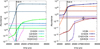 |
Fig. 4 Fractional abundance for B3 fast warm-up (from 10 to 500 K) model at a density of 107 cm−3 for the time period 20 000–35 000 yr with the fiducial model. Oxygen-bearing species are shown to the left and nitrogen bearing to the right. The y-axes have different scales. All species are shown in the key with color-coded dashed horizontal lines showing the observed abundances for B3. The thinner dashed lines indicate the upper limit for HC3 N and the lower limit for C2H5CN, as they are the species that best constrain the time span. The black ellipse highlights the difference between the modeled abundance of C2H5CN and the lower limit of the observed abundance. At the higher densities we tested, the model abundance of C2 H5CN is lower. |
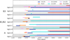 |
Fig. 5 Time periods for which the observed abundances of HC3N, CH3 CN, CH2 CHCN, C2 H5CN, CH3 OCHO, and CH2H5OH are reproduced. The purple “X” marks indicate that the abundance of C2H5CN is not reproduced for this source and gas density. |
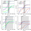 |
Fig. 6 Best fit models of abundances vs. H2 for CH3 OH, C2 H5OH, CH3 CHO, CH3 OCHO, HC3 N, CH3 CN, CH2 CHCN, and C2 H5CN using IC 5. G35.20 B1/B2 (top) is best fit by the fast model with a gas density of 108 cm−3 over a time period of 1.3 kyr. G35.20 A (bottom) is also best fit by the fast model with a gas density of 108 cm−3 over a time period of 6.4 kyr. The line colors for A are the same as B1/B2 as shown in the key. All species are shown in the key with color-coded dashed horizontal lines showing the observed abundances for the source. The thinner dashed lines indicate the upper limit and lower limit species that best constrain the time span. The time ranges in which all abundances can be reproduced within the errors reported in Appendix B are shaded. We truncate the x-axis scale to better highlight the chemistry changes over the temperature range at which the COMs are released from the ice mantles. |
3.2 Reaction–diffusion competition excluded
Reaction–diffusion competition is a mechanism used in chemical modeling to allow grain-surface reactions with energy barriers to proceed more easily. This mechanism compares the relative timescales between the reaction of two species and their diffusion to determine which process will occur (Cuppen et al. 2017). Because reaction–diffusion competition may be overexpressed in a two-phase chemical model (gas and ice), we modeled a test case without it. In this case, key species such as CH3OH, CH3OCHO, and C2 H5OH are underproduced by as much as 2 orders of magnitude compared to the lower limit abundances for any of our observed sources. Figure 7 demonstrates one instance where all three of these species are underproduced for B1-2. More efficient grain-surface chemistry facilitated by reaction–diffusion competition is required to better match the observations, which should be tested in more detailed three-phase chemical models.
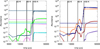 |
Fig. 7 Fractional abundance for B1-2 fast warm-up (from 10 to 500 K) model at a gas density of 107 cm−3 for the time period 5–50 kyr without reaction–diffusion competition. All species are color coded as in Fig. 6 with horizontal lines showing the observed abundances for B1/B2. The abundances of CH3 OH, CH3 OCHO, and C2 H5OH are not reproduced. |
3.3 Varying the initial temperature
It is plausible that for high-mass stars forming in a cluster, possibly sequentially, an initial temperature of 10 K is an underestimation (Tieftrunk et al. 1998). For this reason we also modeled the chemistry of dense gas warming up from 15 to 25 K. Looking at the changes in abundance for constraining species, CH3OCHO, HC3N, and C2 H5CN, we see thatincreasing starting temperatures decrease the abundances of CH3OCHO and C2 H5CN but increase the abundance of HC3N (see Fig. 8). For C2 H5CN, longer timesat as a low temperature allows more to form in the ice, to be later released into the gas phase.
Because the warm-up is exponential, starting at 15 K rather than 10 K results in 6000 years less at a low temperature (and 10 000 for 25 K) for the fast warm-up. Since the formation path to C2 H5CN is mainly in the ice it appears that time at a low temperature is critical. This is demonstrated as well in the medium and slow warm-ups in which high abundances of C2 H5CN are made as these models spend a very long time at low temperatures. The temperature range between 15 and 30 K is critical for grain-surface reactions because the dust temperature determines the sticking efficiency of volatile species (such as H, H2, and CO). At higher temperatures hydrogenation pathways (such as those that lead to C2 H5CN) are less likely to occur.
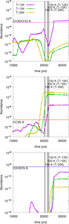 |
Fig. 8 Comparing the fractional abundances for three constraining species, CH3OCHO (top), HC3N (middle), and C2H5CN (bottom), using different initial temperatures (10 K in magenta, 15 K in green, and 25 K in yellow) at a gas density of 107 cm−3 for a fast warm-up. The vertical lines show the time corresponding to a temperature of 100 K for each initial temperature. The observed abundances (horizontal lines) for G35.20 A are shown for reference. |
3.4 Continuing with constant high temperature gas-phase chemistry
To investigate the effect of high temperature gas-phase chemistry on our final abundances in the fast warm-up, we modeled warming up the dense gas to 300 K, then continued at that temperature for an additional 40 kyr. As C2 H5CN is the only species that cannot be fit for source B3, we focus on the abundance of this species produced at different densities with extra time to perform gas-phase chemistry. In Fig. 9, we see that the abundances produced after 300 K do not deviate from those when the gas continues to warm to 500 K. In the extra time, abundances only increase at the highest gas density and then by 36% (~ 1 × 10⁻¹¹), which does not reproduce the observed minimum abundance.
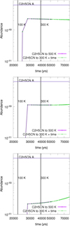 |
Fig. 9 Fractional abundances for C2H5CN comparing warming up to 500 K with warming up to 300 K then continuing at a constant temperature at densities of 107 cm−3 (top), 108 cm−3 (middle), and 109 cm−3 (bottom) fora fast warm-up. The observed abundance (horizontal lines) for G35.20 A is shown for reference. |
3.5 HCN as an initial ice species
HCN has been observed in cometary ice (Mumma & Charnley 2011; Le Roy et al. 2015) and is expected to occur in ices around protostars but has not yet been detected (Boogert et al. 2015). To test the effect of including HCN in the ice, we modeled the following three additional initial abundances of HCN ice: 0.1%, 1%, and 10% vs. H2 O. An abundance of 0.1% reflects the observed abundance in cometary ice (0.08–0.5%), but the higher abundances were used to test if there was any increase in our CN-bearing species using an unrealistic concentration of HCN. In Fig. 10 we see that the constraining species are barely affected by this change in HCN abundance, while the HCN gas abundances are directly affected. We conclude that HCN is not an important progenitor to any of the nitrogen-bearing species that we are focusing on and for the range of physical conditions explored in this work.
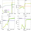 |
Fig. 10 Fractional abundances for nitrogen-bearing species with a gas density of 107 cm−3 and a fast warm-up. HCN gas (solid lines) and ice (dashed lines) abundances with the color key for all four panels (top left), HC3 N gas (top right), CH3CN gas (bottom left), and C2H5CN gas (bottom right) abundances over time are shown for four initial HCN ice abundances (0, 0.1, 1, and 10%). The observed abundances (horizontal lines) for G35.20 A are shown for reference. |
3.6 Varying the cosmic-ray ionization rate
The fiducialmodel uses a low cosmic-ray ionization rate commonly used in chemical modeling of 1.3 × 10⁻¹⁷ s−1, which is low compared with more distant observed star-forming regions (Indriolo et al. 2015). We modeled the chemistry over time for two higher cosmic-ray ionization rates, 1 × 10⁻¹⁶ s−1 and 6 × 10⁻¹⁶ s−1, to be comparable to the mean and uppermost values from Indriolo et al. (2015). When comparing the changes in abundance for constraining species, CH3CN, CH3OCHO, HC3N, and C2 H5CN, we see that a higher cosmic-ray ionization rate increases their abundances, although after ~25 kyr the abundances for a cosmic-ray ionization rate of 6 × 10⁻¹⁶ s−1 drop sharply (see Fig. 11). This sharp drop in our key species is due to either a high abundance of H3 O+ and HNCH+ in the case of CH3CN, CH3OCHO, and HC3N, or dissociation by cosmic rays for C2 H5CN. A cosmic-ray ionization rate of 1 × 10⁻¹⁶ s−1 presents a solution that fits the observed abundances in source B3 with a fast warm-up.
The shortest time period that fits the observed abundances in source B3 is 3.3 kyr in a fast warm-up with a cosmic-ray ionization rate of 1 × 10⁻¹⁶ s−1 and a gas density of 109 cm−3 (Fig. 12). The observed abundances of A and B1-2 are also well fit with a cosmic-ray ionization rate of 1 × 10⁻¹⁶ s−1. A rate of 6 × 10⁻¹⁶ s−1 raises the modeled abundance of HC3N such that itno longer fits any of the observed abundances and so is not a viable solution for the model assumptions and parameters explored here. Table A.1 summarizes the time ranges where the model abundances fit the observed abundances at a cosmic-ray ionization rate of 1 × 10⁻¹⁶ s−1, with corresponding temperatures. It is clear that for the same H2 density and cosmic-ray ionization rate, there is a small time overlap between sources B1/B2 and source B3, and B3 is always a few thousand years older than B1/B2.
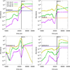 |
Fig. 11 Comparing fractional abundances for four constraining species with different cosmic-ray ionization rates with a gas density of 107 cm−3 for a fast warm-up. CH3CN with the color key for all four panels (top left), HC3N (top right), CH3OCHO (bottom left), and C2H5CN gas (bottom right) abundances over time are shown for three cosmic-ray ionization rates (1.3 × 10⁻¹⁷, 1 × 10⁻¹⁶, and 6 × 10⁻¹⁶ s−1). The observed abundances (horizontal lines) for G35.20 A are shown for reference. |
 |
Fig. 12 Fractional abundances for source B3 with a cosmic-ray ionization rate of 1 × 10⁻¹⁶ s−1, a gas densityof 109 cm−3 for a fast warm-up. All species are shown in the key with color-coded dashed horizontal lines showing the observed abundances for source B3. The thinner dashed lines indicate the upper limit for HC3 N and the lower limit for C2H5CN, as they are the species that constrain the time span. The best fit time period of 3.4 kyr is shaded. The colors are coded as in Fig. 6. |
3.7 Dominant formation routes
We studied the reactions behind each of our eight focus species to determine whether they were formed mostly through ice processing and sublimation, through gas-phase formation following the sublimation of their precursors, or a mixture of both.
CH3OH, HC3N, and C2 H5CN are predominantly produced on the grain surfaces then sublimated with little to no gas-phase production. Significant amounts of CH3CN are produced on the grain surface, but after sublimation gas-phase processes increase the abundance of CH3CN gas to ~8 times the maximum ice abundance. C2 H5OH is also produced predominantly in the ice, but gas processes double the maximum ice abundance.
The ice and gas-phase abundances of CH3CHO are unusual in that the ice abundance drops sharply around 63–70 K in the fast warm-up (at different densities). This appears to coincide with an increase in CH3OH and CH3OCHO gas abundances. At this temperature in the model, grain surface CH3CHO reacts with CH2OH to form either C2 H5OH and HCO orCH3 and CH2OHCHO in the ice, or it reacts with NH2 to form NH3 and CH3CO in the ice as well. CH2OHCHO is important in forming CH3OH and CH3OCHO on grain surfaces. The CH3CHO gas abundance does not increase until the temperature reaches ~100 K. At that temperature, the main production pathway is through neutral-neutral reactions between CH3OH and CH in the gas phase. So despite the significant abundances of CH3CHO that are produced in the ice, very little of this sublimates into the gas phase. The CH3CHO gas is mainly a product of CH3OH and CH.
CH3OCHO is made abundantly in the ice, but reacts with OH in the ice to form COOCH3 and water ice by hydrogen abstraction. COOCH3 is hydrogenated in the ice and the resulting CH3OCHO is released to the gas (H(ice) + COOCH3(ice) = CH3OCHO). This is the main mechanism for creating CH3OCHO in the gas rather than sublimation of CH3OCHO from the ice or formation in the gas.
CH2CHCN is another species that can be made at low fractional abundances (10−12–10−10) in the ice and gas. Ice phase CH2CHCN is dominantly produced through the dissociation of C2 H5CN by cosmic rays, whereas the gas-phase formation route is the reaction of CN with either C2 H4 or CH3CHCH2. After a temperature of ~115 K, the CH2CHCN in the ice is sublimated and adds to the gas-phase abundance.
4 Discussion
4.1 General test differences
The first interesting result is that our model abundances are almost independent of initial ice conditions that we used, which are constrained by the observations of Gibb et al. (2004) and theoretical abundance ratios from van Dishoeck (2004). The range of ice abundances in our different IC sets is not large, but it is based on real sources. The models suggest that the initial ice composition is not crucial to modeling the chemical composition of a later state, thereby showing that the warm-up stage determines the composition of the hot core. It is possible that adding molecular gas to the initial conditions would have an effect on the final abundances; however, such a parameter-space exploration of the initial gas composition requires a dedicated suite of models and is beyond the scope of this work. This should be carried out in the future.
The second interesting result is a much debated topic in chemical modeling (Cuppen et al. 2017): the importance of approximating reaction–diffusion competition in rate equation based models. In this work, in order to reproduce the lower limit abundances of the species that we focus on from G35.20, reaction–diffusion competition is needed, otherwise oxygen-bearing complex organic species are underproduced by as much as 2 orders of magnitude. Reaction–diffusion competition has also been shown to be necessary in the work of Ruaud et al. (2016) and Quénard et al. (2018) among others, but it is important to note that gas-phase reactions for COMs in chemical networks have also been shown to be incomplete (Balucani et al. 2015).
The modeled gas temperatures at which the abundances are reproduced are lower than the kinetic temperatures (300 K for source B3, 285 K for core A, 160 K for source B1, 120 K for source B2) determined in Allen et al. (2017). The gas temperatures from our chemical model are 110-130 K for source B3, 100-110 K for sources B1/B2, and 100-130 K for core A. As we have demonstrated that increasing the temperature and running the chemistry for longer does not significantly affect the final abundances, then the reproduction of the observed abundances at lower temperatures is an advantage.
4.2 Reproducing source B3
In our fiducial model, the warm-up time is the most significant factor in reproducing the abundances of the observed species. The high abundances of C2 H5CN seen in source B3 cannot be produced in a fast warm-up in our fiducial model. While relatively short time ranges can be found to reproduce the abundances seen in sources B1/B2 in any of our models (with the shortest time range of 1.3 kyr from a fast model at 108 cm−3), those of source B3 can only be reproduced in medium or slow warm-up models. These longer warm-up times imply a lower mass protostar. Observational evidence points to source B3 being associated with a high-mass protostar: there are numerous masers about its position and the kinetic temperature is high (~300 K). On the other hand, a high deuterium fraction (13%) for CH3CN (Allen et al. 2017) indicates that it was recently very cold and therefore needs a faster warm-up time.
We reproduced the observed abundances in source B3 well using a cosmic-ray ionization rate a few times higher than in the standard value (van der Tak & van Dishoeck 2000) for the interstellar medium. A higher mean cosmic-ray ionization rate of 1.78 × 10⁻¹⁶ s−1 was found in observations by Indriolo et al. (2015) and our models seem to agree with this higher rate. Source B1/B2 is also well reproduced within a 1.3 kyr time period using a cosmic-ray ionization rate of 1 × 10⁻¹⁶ s−1, without the abundances of the complex cyanides becoming too high.
It is possible that adding gas-phase reactions forming C2 H5CN to the network will make it possible to reproduce the higher abundances seen in source B3 with the fiducial model, as the network currently contains no gas-phase reactions to produce this species. Such reactions are not often tested in the laboratory as cyanides are dangerous to work with, but it would be extremely useful for labs to test these reactions in the future to improve the chemical networks.
4.3 Warm-up times
The Garrod models (Garrod & Herbst 2006; Garrod et al. 2008) and their predecessor models (Viti & Williams 1999) derive their warm-up times from the work of Bernasconi & Maeder (1996; BM96 from here on). In BM96 work, the contraction times for different masses of stars (from 0.8 to 60 M⊙) are determined under the assumption that the accretion rate is between 10−5 and 10−4 M⊙ yr−1. It has been reported more recently that mass accretion rates can be as high as 10−3 M⊙ yr−1 (Tan et al. 2014), although this may be episodic. Hosokawa & Omukai (2009) found that these high accretion rates led to pre-main sequence stars with larger-than-typical radii. Ramírez-Tannus et al. (2017) has recently reported observational evidence for this in M17. In any case, our fast, medium, and slow warm-up times correspond to 60, 15, and 6 M⊙ objects from the original BM96 paper, considered to be very high, high, and intermediate mass sources. If we assume that the accretion rate of our objects is ten times higher and decrease the contraction times of the BM96 objects accordingly, that gives more reasonable stellar masses of 8, 4, and 1 M⊙ for the fast, medium, and slow warm ups, respectively. This is not a strictly accurate way of determining the relationship between mass at warm-up time, but it leads to much more reasonable masses and takes into account the observational and theoretical work that has been carried out since BM96 was published.
5 Conclusions
The disagreement between the disk-like kinematics of the high-mass star-forming region in G35.20−0.74 B and its chemical segregation across its individual cores is not easily explained. The high cyanide abundances observed toward peak B3 can be reproduced in a fast warm-up, but only with a higher cosmic-ray ionization rate of 1 × 10⁻¹⁶ s−1. The smallest time period required to reproduce the abundances in source B3 is 3.3 kyr at a gas density of 109 cm−3. This is a reasonable cosmic-ray ionization rate as evidenced by observations by Indriolo et al. (2015). The abundances observed in the rest of the disk candidate (B1/B2) can easily be reproduced with a fast warm-up at a gas density of 108 cm−3 and a low rate of cosmic-ray ionization in a very short time period (~1.3 kyr), but can also be reproduced with the higher cosmic-ray ionization rate of 1 × 10⁻¹⁶ s−1 at a gas density of 109 cm−3 in 1.3 kyr.
We find that the abundance of ethyl cyanide in particular is maximized in models with a low initial temperature, a high cosmic-ray ionization rate, a long warm-up time, or a lower gas density. The model is most sensitive to age in the context of a warm-up model (therefore temperature), and to cosmic-ray ionization rate. It is not sensitive to the initial ice composition (within observed ranges) and not strongly dependent on gas density showing that the warm-up phase determines the composition.
If we assume that the cosmic-ray ionization rate is the same around sources B1/B2 and source B3 at 1 × 10⁻¹⁶ s−1 and the sources have a gas density of 109 cm−3, then the age of sources B1/B2 is 22.3–23.6 kyr while the age of source B3 is 22.7–26 kyr. This indicates that both these sources began forming within a few thousand years and source B3 is 2000 years older. Based on an outer disk rotation period between 9700 and 11 100 years, this age difference is physically possible. So we conclude that the detection of CH2CHCN and C2 H5CN can indicate a lower limit for the age of a hot core and a nondetection indicates an upper age limit. This can be useful when observing a potential multiple system at a lower resolution, where if CH2CHCN or C2 H5CN is detected toward one part of a source and undetected in others, it indicates a young high-mass system with protostars of different ages.
We have covered a variety of star formation scenarios including a range of gas densities, regions with triggered star formation (starting at temperatures above 10 K), regions with higher and lower cosmic-ray ionization rates, and a range of masses (via warm-up speeds). With this coverage of parameter space we propose that these model results can be used to interpret and predict observations from a variety of embedded high-mass sources and intend to investigate other sources in the future. While we have explored the parameter space in these models comprehensively and noted the trends arising from this analysis, there is still much work to be carried out theoretically and experimentally to understand the gas and ice chemistry of cyanides. Without this work, our ability to study complex cyanide chemistry will remain hindered.
Time ranges (in kyr) that are needed fit observed abundances in the lower abundance sources, B1/B2, those for the higher abundance source, B3, at a cosmic-ray ionization rate of 1 × 10⁻¹⁶ s−1 in a fast warm up.
Acknowledgements
We would like to thank our referee, Professor Serena Viti, for her constructive comments and quick reading. The PhD project of V. Allen is funded by the Netherlands Organisation for Scientific Research (NWO) and Netherlands Institute for Space Research (SRON). C. Walsh acknowledges NWO (program 639.041.335) and the University of Leeds for financial support.
Appendix A: Initial conditions
Full initial conditions (abundance of each species vs. total composition).
Appendix B: Abundance ranges with errors
Abundance range observed in Allen et al. (2017).
Appendix C: Comparison with Garrod et al. (2008)
We compared our model without reaction–diffusion competition to the well-known model in Garrod et al. (2008) and found significant differences. At all warm-up speeds the difference between our abundances and their reduced model is 1 to 4 orders of magnitude for more complex species, while the abundances of simpler species (H2 O, CO, NH3, and CH4) are similar to those in Garrod et al. (2008). The model abundances from Garrod et al. (2008) cannot reproduce the observed abundances in G35.20 B3, as the fractional abundances of C2 H5OH, CH3OCHO, and CH3CHO are at least one order of magnitude too low. These authors did not report abundances of CH2CHCN or C2 H5CN so that cannot be compared. There are some notable differences between our model results and those of Garrod. The initial ice composition not the same, although we found that the initial ice composition does not strongly affect the final abundances. Without knowing their grain-surface parameters, that cannot be compared. Garrod et al. also used a different gas network from us (UMIST vs. OSU) and both networks have been updated significantly since 2008. Most updates to the networks involve updating the binding energies of surface species (Penteado et al. 2017). We also take further steps in varying the cosmic-ray ionization rate and gas densities to investigate the effect of these parameters on the chemical make-up of our modeled sources.
Appendix D: Time ranges
Tables and figures showing the time ranges that are required to reproduce observed abundances within errors.
Approximate time period (in years) during which the modeled abundance range matches the observed abundance range for B3.
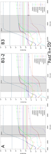 |
Fig. D.1 Abundances vs. H2 for CH3OH, C2 H5OH, CH3 CHO, CH3 OCHO, HC3 N, CH3 CN, CH2 CHCN, and C2H5CN using IC 5 with a density of 107 cm−3 and a fast warm-up time of 50 kyr are shown for G35.20 A (left), B1/B2 (middle), and B3 (right). The time period shown is only a part of the modeled time, from 180 00 to 35 000 yr. The time range in which all abundancescan be reproduced with an error of 1 order of magnitude are shaded in gray. The abundance of C2 H5CN in B3 is not reproduced so a small black ellipse shows the gap between the lower abundance limit and the modeled abundance. |
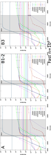 |
Fig. D.2 Abundances vs. H2 for CH3OH, C2 H5OH, CH3 CHO, CH3 OCHO, HC3 N, CH3 CN, CH2 CHCN, and C2H5CN using IC 5 with a density of 108 cm−3 and a fast warm-up time of 50 kyr are shown for G35.20 A (left), B1/B2 (middle), and B3 (right). The time period shown is only a part of the modeled time, from 18 000 to 35 000 yr. The time range in which all abundancescan be reproduced with an error of 1 order of magnitude are shaded in gray. The abundance of C2 H5CN in B3 is not reproduced so a small black ellipse shows the gap between the lower abundance limit and the modeled abundance. |
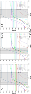 |
Fig. D.3 Abundances vs. H2 for CH3OH, C2 H5OH, CH3 CHO, CH3 OCHO, HC3 N, CH3 CN, CH2 CHCN, and C2H5CN using IC 5 with a density of 109 cm−3 and a fast warm-up time of 50 kyr are shown for G35.20 A (left), B1/B2 (middle), and B3 (right). The time period shown is only a part of the modeled time, from 18 000 to 35 000 yr. The time range in which all abundancescan be reproduced with an error of 1 order of magnitude are shaded in gray. The abundance of C2 H5CN in A and B3 is not reproduced so a small black ellipse shows the gap between the lower abundance limit and the modeled abundance. |
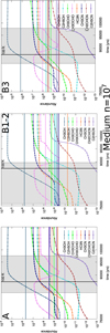 |
Fig. D.4 Abundances vs. H2 for CH3OH, C2 H5OH, CH3 CHO, CH3 OCHO, HC3 N, CH3 CN, CH2 CHCN, and C2H5CN using IC 5 with a density of 107 cm−3 and a medium warm-up time of 200 kyr are shown for G35.20 A (left), B1/B2 (middle), and B3 (right). The time period shown is only a part of the modeled time, from 70 to 120 kyr for A and B3 and 30–105 kyr for B1/B2. The time range in which all abundances can be reproduced with an error of 1 order of magnitude are shaded in gray. |
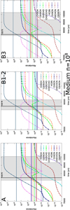 |
Fig. D.5 Abundances vs. H2 for CH3OH, C2 H5OH, CH3 CHO, CH3 OCHO, HC3 N, CH3 CN, CH2 CHCN, and C2H5CN using IC 5 with a density of 108 cm−3 and a medium warm-up time of 200 kyr are shown for G35.20 A (left), B1/B2 (middle), and B3 (right). The time period shown is only a part of the modeled time, from 70 to 120 kyr for A and B3 and 30–105 kyr for B1/B2. The time range in which all abundances can be reproduced with an error of 1 order of magnitude are shaded in gray. The abundance of C2 H5CN in B3 is not reproduced. |
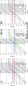 |
Fig. D.6 Abundances vs. H2 for CH3OH, C2 H5OH, CH3 CHO, CH3 OCHO, HC3 N, CH3 CN, CH2 CHCN, and C2H5CN using IC 5 with a density of 109 cm−3 and a medium warm-up time of 200 kyr are shown for G35.20 A (left), B1/B2 (middle), and B3 (right). The time period shown is only a part of the modeled time, from 70 to 120 kyr for A and B3 and 30–105 kyr for B1/B2. The time range in which all abundances can be reproduced with an error of 1 order of magnitude are shaded in gray. The abundance of C2 H5CN in B3 is not reproduced. |
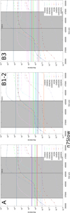 |
Fig. D.7 Abundances vs. H2 for CH3OH, C2 H5OH, CH3 CHO, CH3 OCHO, HC3 N, CH3 CN, CH2 CHCN, and C2H5CN using IC 5 with a density of 107 cm−3 and a slow warm-up time of 1 Myr are shown for G35.20 A (left), B1/B2 (middle), and B3 (right). The time period shown is only a part of the modeled time, from 350 to 510 kyr. The time range in which all abundances can be reproduced with an error of 1 order of magnitude are shaded in gray. |
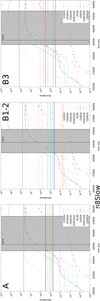 |
Fig. D.8 Abundances vs. H2 for CH3OH, C2 H5OH, CH3 CHO, CH3 OCHO, HC3 N, CH3 CN, CH2 CHCN, and C2H5CN using IC 5 with a density of 107 cm−3 and a slow warm-up time of 1 Myr are shown for G35.20 A (left), B1/B2 (middle), and B3 (right). The time period shown is only a part of the modeled time, from 350 to 510 kyr. The time range in which all abundances can be reproduced with an error of 1 order of magnitude are shaded in gray. |
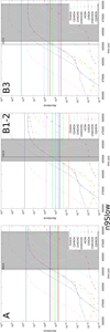 |
Fig. D.9 Abundances vs. H2 for CH3OH, C2 H5OH, CH3 CHO, CH3 OCHO, HC3 N, CH3 CN, CH2 CHCN, and C2H5CN using IC 5 with a density of 109 cm−3 and a slow warm-up time of 1 Myr are shown for G35.20 A (left), B1/B2 (middle), and B3 (right). The time period shown is only a part of the modeled time, from 350 to 510 kyr. The time range in which all abundances can be reproduced with an error of 1 order of magnitude are shaded in gray. |
References
- Allen, V., van der Tak, F. F. S., Sánchez-Monge, Á., Cesaroni, R., & Beltrán, M. T. 2017, A&A, 603, A133 [NASA ADS] [CrossRef] [EDP Sciences] [Google Scholar]
- Balucani, N., Ceccarelli, C., & Taquet, V. 2015, MNRAS, 449, L16 [Google Scholar]
- Bernasconi, P. A., & Maeder, A. 1996, A&A, 307, 829 [NASA ADS] [Google Scholar]
- Blake, G. A., Sutton, E. C., Masson, C. R., & Phillips, T. G. 1987, ApJ, 315, 621 [NASA ADS] [CrossRef] [Google Scholar]
- Boogert, A. C. A., Gerakines, P. A., & Whittet, D. C. B. 2015, ARA&A, 53, 541 [Google Scholar]
- Caselli, P., Hasegawa, T. I., & Herbst, E. 1993, ApJ, 408, 548 [NASA ADS] [CrossRef] [Google Scholar]
- Crockett, N. R., Bergin, E. A., Neill, J. L., et al. 2015, ApJ, 806, 239 [NASA ADS] [CrossRef] [Google Scholar]
- Cuppen, H. M., Walsh, C., Lamberts, T., et al. 2017, Space Sci. Rev., 212, 1 [NASA ADS] [CrossRef] [Google Scholar]
- Drozdovskaya, M. N., Walsh, C., Visser, R., Harsono, D., & van Dishoeck E. F. 2014, MNRAS, 445, 913 [NASA ADS] [CrossRef] [Google Scholar]
- Feng, S., Beuther, H., Henning, T., et al. 2015, A&A, 581, A71 [NASA ADS] [CrossRef] [EDP Sciences] [Google Scholar]
- Garrod, R. T., & Herbst, E. 2006, A&A, 457, 927 [NASA ADS] [CrossRef] [EDP Sciences] [Google Scholar]
- Garrod, R. T., Widicus Weaver, S. L., & Herbst, E. 2008, ApJ, 682, 283 [NASA ADS] [CrossRef] [Google Scholar]
- Gibb, E. L., Whittet, D. C. B., Boogert, A. C. A., & Tielens, A. G. G. M. 2004, ApJS, 151, 35 [NASA ADS] [CrossRef] [PubMed] [Google Scholar]
- Herbst, E., & van Dishoeck E. F. 2009, ARA&A, 47, 427 [NASA ADS] [CrossRef] [Google Scholar]
- Hosokawa, T., & Omukai, K. 2009, ApJ, 691, 823 [NASA ADS] [CrossRef] [Google Scholar]
- Hutawarakorn, B., & Cohen, R. J. 1999, MNRAS, 303, 845 [NASA ADS] [CrossRef] [Google Scholar]
- Indriolo, N., Neufeld, D. A., Gerin, M., et al. 2015, ApJ, 800, 40 [NASA ADS] [CrossRef] [Google Scholar]
- Jiménez-Serra, I., Zhang, Q., Viti, S., Martín-Pintado, J., & de Wit W.-J. 2012, ApJ, 753, 34 [NASA ADS] [CrossRef] [Google Scholar]
- Koumpia, E., van der Tak, F. F. S., Kwon, W., et al. 2016, A&A, 595, A51 [NASA ADS] [CrossRef] [EDP Sciences] [Google Scholar]
- Le Roy, L., Altwegg, K., Balsiger, H., et al. 2015, A&A, 583, A1 [Google Scholar]
- McElroy, D., Walsh, C., Markwick, A. J., et al. 2013, A&A, 550, A36 [NASA ADS] [CrossRef] [EDP Sciences] [Google Scholar]
- Möller, T., Endres, C., & Schilke, P. 2017, A&A, 598, A7 [NASA ADS] [CrossRef] [EDP Sciences] [Google Scholar]
- Mumma, M. J., & Charnley, S. B. 2011, ARA&A, 49, 471 [NASA ADS] [CrossRef] [Google Scholar]
- Penteado, E. M., Walsh, C., & Cuppen, H. M. 2017, ApJ, 844, 71 [NASA ADS] [CrossRef] [Google Scholar]
- Quénard, D., Jiménez-Serra, I., Viti, S., Holdship, J., & Coutens, A. 2018, MNRAS, 474, 2796 [NASA ADS] [CrossRef] [Google Scholar]
- Ramírez-Tannus, M. C., Kaper, L., de Koter, A., et al. 2017, A&A, 604, A78 [NASA ADS] [CrossRef] [EDP Sciences] [Google Scholar]
- Ruaud, M., Wakelam, V., & Hersant, F. 2016, MNRAS, 459, 3756 [NASA ADS] [CrossRef] [Google Scholar]
- Ruoskanen, J., Harju, J., Juvela, M., et al. 2011, A&A, 534, A122 [NASA ADS] [CrossRef] [EDP Sciences] [Google Scholar]
- Sánchez-Monge, Á., Cesaroni, R., Beltrán, M. T., et al. 2013, A&A, 552, L10 [NASA ADS] [CrossRef] [EDP Sciences] [Google Scholar]
- Sánchez-Monge, Á., Beltrán, M. T., Cesaroni, R., et al. 2014, A&A, 569, A11 [NASA ADS] [CrossRef] [EDP Sciences] [Google Scholar]
- Tan, J. C., Beltrán, M. T., Caselli, P., et al. 2014, Protostars and Planets VI, eds. H. Beuther, R. S. Klessen, C. P. Dullemond, & T. Henning (Tucson: University of Arizona Press), 149 [Google Scholar]
- Tieftrunk, A. R., Gaume, R. A., & Wilson, T. L. 1998, A&A, 340, 232 [NASA ADS] [Google Scholar]
- van der Tak, F. F. S., & van Dishoeck E. F. 2000, A&A, 358, L79 [NASA ADS] [Google Scholar]
- van Dishoeck, E. F. 2004, ARA&A, 42, 119 [NASA ADS] [CrossRef] [Google Scholar]
- Vastel, C., Ceccarelli, C., Lefloch, B., & Bachiller, R. 2016, A&A, 591, L2 [NASA ADS] [CrossRef] [EDP Sciences] [Google Scholar]
- Viti, S., & Williams, D. A. 1999, MNRAS, 305, 755 [NASA ADS] [CrossRef] [Google Scholar]
- Viti, S., Collings, M. P., Dever, J. W., McCoustra, M. R. S., & Williams, D. A. 2004, MNRAS, 354, 1141 [NASA ADS] [CrossRef] [Google Scholar]
- Walsh, C., Millar, T. J., Nomura, H., et al. 2014, A&A, 563, A33 [NASA ADS] [CrossRef] [EDP Sciences] [Google Scholar]
- Walsh, C., Nomura, H., & van Dishoeck E. 2015, A&A, 582, A88 [NASA ADS] [CrossRef] [EDP Sciences] [Google Scholar]
- Wyrowski, F., Schilke, P., Walmsley, C. M., & Menten, K. M. 1999, ApJ, 514, L43 [NASA ADS] [CrossRef] [Google Scholar]
All Tables
Time ranges (in kyr) that fit observed abundances using the fiducial model in the lower abundance sources, B1/B2, those for the higher abundance source, B3, and the other hot core in this group, A.
Time ranges (in kyr) that are needed fit observed abundances in the lower abundance sources, B1/B2, those for the higher abundance source, B3, at a cosmic-ray ionization rate of 1 × 10⁻¹⁶ s−1 in a fast warm up.
Approximate time period (in years) during which the modeled abundance range matches the observed abundance range for B3.
All Figures
|
Fig. 1 870 μm continuum emission from Cycle 0 ALMA observations of G35.20. The continuum peaks are labeled in order of intensity (i.e., peak B1 has the highest and peak B3 the lowest continuum intensity). Contour levels are 0.03, 0.042, 0.055, 0.067, 0.08, 0.10, 0.13, 0.18, and 0.23 Jy beam−1 (σ = 1.8 mJy beam−1). The pixel-sized colored squares denote each of the spectral extraction points (from Allen et al. 2017). |
| In the text | |
|
Fig. 2 Abundances of simple species over time for a fast warm-up with a gas density of 107 cm−3. Dashed lines show ice abundances and solid lines show gas abundances. |
| In the text | |
|
Fig. 3 Fractional abundance vs. H2 for one species with different initial conditions (ICs 1-5) for a gas density of 107 cm−3 and a fast warm-up time of 50 kyr. Results are similar for other warm-up times and densities. |
| In the text | |
|
Fig. 4 Fractional abundance for B3 fast warm-up (from 10 to 500 K) model at a density of 107 cm−3 for the time period 20 000–35 000 yr with the fiducial model. Oxygen-bearing species are shown to the left and nitrogen bearing to the right. The y-axes have different scales. All species are shown in the key with color-coded dashed horizontal lines showing the observed abundances for B3. The thinner dashed lines indicate the upper limit for HC3 N and the lower limit for C2H5CN, as they are the species that best constrain the time span. The black ellipse highlights the difference between the modeled abundance of C2H5CN and the lower limit of the observed abundance. At the higher densities we tested, the model abundance of C2 H5CN is lower. |
| In the text | |
|
Fig. 5 Time periods for which the observed abundances of HC3N, CH3 CN, CH2 CHCN, C2 H5CN, CH3 OCHO, and CH2H5OH are reproduced. The purple “X” marks indicate that the abundance of C2H5CN is not reproduced for this source and gas density. |
| In the text | |
|
Fig. 6 Best fit models of abundances vs. H2 for CH3 OH, C2 H5OH, CH3 CHO, CH3 OCHO, HC3 N, CH3 CN, CH2 CHCN, and C2 H5CN using IC 5. G35.20 B1/B2 (top) is best fit by the fast model with a gas density of 108 cm−3 over a time period of 1.3 kyr. G35.20 A (bottom) is also best fit by the fast model with a gas density of 108 cm−3 over a time period of 6.4 kyr. The line colors for A are the same as B1/B2 as shown in the key. All species are shown in the key with color-coded dashed horizontal lines showing the observed abundances for the source. The thinner dashed lines indicate the upper limit and lower limit species that best constrain the time span. The time ranges in which all abundances can be reproduced within the errors reported in Appendix B are shaded. We truncate the x-axis scale to better highlight the chemistry changes over the temperature range at which the COMs are released from the ice mantles. |
| In the text | |
|
Fig. 7 Fractional abundance for B1-2 fast warm-up (from 10 to 500 K) model at a gas density of 107 cm−3 for the time period 5–50 kyr without reaction–diffusion competition. All species are color coded as in Fig. 6 with horizontal lines showing the observed abundances for B1/B2. The abundances of CH3 OH, CH3 OCHO, and C2 H5OH are not reproduced. |
| In the text | |
|
Fig. 8 Comparing the fractional abundances for three constraining species, CH3OCHO (top), HC3N (middle), and C2H5CN (bottom), using different initial temperatures (10 K in magenta, 15 K in green, and 25 K in yellow) at a gas density of 107 cm−3 for a fast warm-up. The vertical lines show the time corresponding to a temperature of 100 K for each initial temperature. The observed abundances (horizontal lines) for G35.20 A are shown for reference. |
| In the text | |
|
Fig. 9 Fractional abundances for C2H5CN comparing warming up to 500 K with warming up to 300 K then continuing at a constant temperature at densities of 107 cm−3 (top), 108 cm−3 (middle), and 109 cm−3 (bottom) fora fast warm-up. The observed abundance (horizontal lines) for G35.20 A is shown for reference. |
| In the text | |
|
Fig. 10 Fractional abundances for nitrogen-bearing species with a gas density of 107 cm−3 and a fast warm-up. HCN gas (solid lines) and ice (dashed lines) abundances with the color key for all four panels (top left), HC3 N gas (top right), CH3CN gas (bottom left), and C2H5CN gas (bottom right) abundances over time are shown for four initial HCN ice abundances (0, 0.1, 1, and 10%). The observed abundances (horizontal lines) for G35.20 A are shown for reference. |
| In the text | |
|
Fig. 11 Comparing fractional abundances for four constraining species with different cosmic-ray ionization rates with a gas density of 107 cm−3 for a fast warm-up. CH3CN with the color key for all four panels (top left), HC3N (top right), CH3OCHO (bottom left), and C2H5CN gas (bottom right) abundances over time are shown for three cosmic-ray ionization rates (1.3 × 10⁻¹⁷, 1 × 10⁻¹⁶, and 6 × 10⁻¹⁶ s−1). The observed abundances (horizontal lines) for G35.20 A are shown for reference. |
| In the text | |
|
Fig. 12 Fractional abundances for source B3 with a cosmic-ray ionization rate of 1 × 10⁻¹⁶ s−1, a gas densityof 109 cm−3 for a fast warm-up. All species are shown in the key with color-coded dashed horizontal lines showing the observed abundances for source B3. The thinner dashed lines indicate the upper limit for HC3 N and the lower limit for C2H5CN, as they are the species that constrain the time span. The best fit time period of 3.4 kyr is shaded. The colors are coded as in Fig. 6. |
| In the text | |
|
Fig. D.1 Abundances vs. H2 for CH3OH, C2 H5OH, CH3 CHO, CH3 OCHO, HC3 N, CH3 CN, CH2 CHCN, and C2H5CN using IC 5 with a density of 107 cm−3 and a fast warm-up time of 50 kyr are shown for G35.20 A (left), B1/B2 (middle), and B3 (right). The time period shown is only a part of the modeled time, from 180 00 to 35 000 yr. The time range in which all abundancescan be reproduced with an error of 1 order of magnitude are shaded in gray. The abundance of C2 H5CN in B3 is not reproduced so a small black ellipse shows the gap between the lower abundance limit and the modeled abundance. |
| In the text | |
|
Fig. D.2 Abundances vs. H2 for CH3OH, C2 H5OH, CH3 CHO, CH3 OCHO, HC3 N, CH3 CN, CH2 CHCN, and C2H5CN using IC 5 with a density of 108 cm−3 and a fast warm-up time of 50 kyr are shown for G35.20 A (left), B1/B2 (middle), and B3 (right). The time period shown is only a part of the modeled time, from 18 000 to 35 000 yr. The time range in which all abundancescan be reproduced with an error of 1 order of magnitude are shaded in gray. The abundance of C2 H5CN in B3 is not reproduced so a small black ellipse shows the gap between the lower abundance limit and the modeled abundance. |
| In the text | |
|
Fig. D.3 Abundances vs. H2 for CH3OH, C2 H5OH, CH3 CHO, CH3 OCHO, HC3 N, CH3 CN, CH2 CHCN, and C2H5CN using IC 5 with a density of 109 cm−3 and a fast warm-up time of 50 kyr are shown for G35.20 A (left), B1/B2 (middle), and B3 (right). The time period shown is only a part of the modeled time, from 18 000 to 35 000 yr. The time range in which all abundancescan be reproduced with an error of 1 order of magnitude are shaded in gray. The abundance of C2 H5CN in A and B3 is not reproduced so a small black ellipse shows the gap between the lower abundance limit and the modeled abundance. |
| In the text | |
|
Fig. D.4 Abundances vs. H2 for CH3OH, C2 H5OH, CH3 CHO, CH3 OCHO, HC3 N, CH3 CN, CH2 CHCN, and C2H5CN using IC 5 with a density of 107 cm−3 and a medium warm-up time of 200 kyr are shown for G35.20 A (left), B1/B2 (middle), and B3 (right). The time period shown is only a part of the modeled time, from 70 to 120 kyr for A and B3 and 30–105 kyr for B1/B2. The time range in which all abundances can be reproduced with an error of 1 order of magnitude are shaded in gray. |
| In the text | |
|
Fig. D.5 Abundances vs. H2 for CH3OH, C2 H5OH, CH3 CHO, CH3 OCHO, HC3 N, CH3 CN, CH2 CHCN, and C2H5CN using IC 5 with a density of 108 cm−3 and a medium warm-up time of 200 kyr are shown for G35.20 A (left), B1/B2 (middle), and B3 (right). The time period shown is only a part of the modeled time, from 70 to 120 kyr for A and B3 and 30–105 kyr for B1/B2. The time range in which all abundances can be reproduced with an error of 1 order of magnitude are shaded in gray. The abundance of C2 H5CN in B3 is not reproduced. |
| In the text | |
|
Fig. D.6 Abundances vs. H2 for CH3OH, C2 H5OH, CH3 CHO, CH3 OCHO, HC3 N, CH3 CN, CH2 CHCN, and C2H5CN using IC 5 with a density of 109 cm−3 and a medium warm-up time of 200 kyr are shown for G35.20 A (left), B1/B2 (middle), and B3 (right). The time period shown is only a part of the modeled time, from 70 to 120 kyr for A and B3 and 30–105 kyr for B1/B2. The time range in which all abundances can be reproduced with an error of 1 order of magnitude are shaded in gray. The abundance of C2 H5CN in B3 is not reproduced. |
| In the text | |
|
Fig. D.7 Abundances vs. H2 for CH3OH, C2 H5OH, CH3 CHO, CH3 OCHO, HC3 N, CH3 CN, CH2 CHCN, and C2H5CN using IC 5 with a density of 107 cm−3 and a slow warm-up time of 1 Myr are shown for G35.20 A (left), B1/B2 (middle), and B3 (right). The time period shown is only a part of the modeled time, from 350 to 510 kyr. The time range in which all abundances can be reproduced with an error of 1 order of magnitude are shaded in gray. |
| In the text | |
|
Fig. D.8 Abundances vs. H2 for CH3OH, C2 H5OH, CH3 CHO, CH3 OCHO, HC3 N, CH3 CN, CH2 CHCN, and C2H5CN using IC 5 with a density of 107 cm−3 and a slow warm-up time of 1 Myr are shown for G35.20 A (left), B1/B2 (middle), and B3 (right). The time period shown is only a part of the modeled time, from 350 to 510 kyr. The time range in which all abundances can be reproduced with an error of 1 order of magnitude are shaded in gray. |
| In the text | |
|
Fig. D.9 Abundances vs. H2 for CH3OH, C2 H5OH, CH3 CHO, CH3 OCHO, HC3 N, CH3 CN, CH2 CHCN, and C2H5CN using IC 5 with a density of 109 cm−3 and a slow warm-up time of 1 Myr are shown for G35.20 A (left), B1/B2 (middle), and B3 (right). The time period shown is only a part of the modeled time, from 350 to 510 kyr. The time range in which all abundances can be reproduced with an error of 1 order of magnitude are shaded in gray. |
| In the text | |
Current usage metrics show cumulative count of Article Views (full-text article views including HTML views, PDF and ePub downloads, according to the available data) and Abstracts Views on Vision4Press platform.
Data correspond to usage on the plateform after 2015. The current usage metrics is available 48-96 hours after online publication and is updated daily on week days.
Initial download of the metrics may take a while.