| Issue |
A&A
Volume 615, July 2018
|
|
|---|---|---|
| Article Number | A174 | |
| Number of page(s) | 11 | |
| Section | Interstellar and circumstellar matter | |
| DOI | https://doi.org/10.1051/0004-6361/201832769 | |
| Published online | 07 August 2018 | |
Optimal extinction measurements
I. Single-object extinction inference
Department of Physics, University of Milan, via Celoria 16, 20133 Milan, Italy
e-mail: This email address is being protected from spambots. You need JavaScript enabled to view it.
Received:
5
February
2018
Accepted:
23
April
2018
Abstract
In this paper we present XNICER, an optimized multi-band extinction technique based on the extreme deconvolution of the intrinsic colors of objects observed through a molecular cloud. XNICER follows a rigorous statistical approach and provides the full Bayesian inference of the extinction for each observed object. Photometric errors in both the training control field and in the science field are properly taken into account. XNICER improves over the known extinction methods and is computationally fast enough to be used on large datasets of objects. Our tests and simulations show that this method is able to reduce the noise associated with extinction measurements by a factor 2 with respect to the previous NICER algorithm, and it has no evident bias even at high extinctions.
Key words: ISM: clouds / dust, extinction / ISM: structure / methods: statistical
© ESO 2018
1. Introduction
Understanding the anatomy of molecular clouds is critical to decipher the process of star and planet formation. However, since molecular clouds are mainly composed of cold (~10 K) molecular hydrogen and helium, which are virtually invisible, studies of these objects have to rely on rare tracers and extrapolate their small abundancies to obtain the full mass distribution.
Of the techniques that are used to study molecular clouds, the ones based on optical and infrared extinction are probably the most consistent (Goodman et al. 2009). They are based on what is widely thought to be the most reliable gas tracer at our disposal: dust. Moreover, they use a very small set of assumptions and are free from many of the uncertainties that plague other methods. Infrared extinction, in particular, has been successfully employed to investigate the interstellar medium at many different scales: from small cores (e.g. Alves et al. 2001), to giant molecular clouds (Lombardi et al. 2010), to the entire sky (using star counts, as described by Dobashi 2011 and Dobashi et al. 2013, or color excess, as described by Juvela & Montillaud 2016a).
Extinction measurements are not only powerful per se: they are also often used to calibrate other techniques, so as to reduce many uncertainties. For example, submillimeter dust emission observations can be used to produce exquisite dust emission maps, which often present spectacular views of entire molecular clouds at relatively high resolution. These maps, however, would be scientifically of little use without a proper calibration, which is often achieved using (lower resolution) extinction maps of the same area (e.g. Lombardi et al. 2014; Zari et al. 2016). Similarly, extinction is used to calibrate maps of near-infrared scattered light (Juvela et al. 2006; see also, e.g. Malinen et al. 2013). Finally, extinction is crucial also to infer the X-factor of radio observations of different molecules.
As early recognized by Lada et al. (1994), extinction is best measured from the color excess of background stars. Most studies since then have been carried out in the near-infrared (NIR), because at these wavelengths molecular clouds are more transparent than at visible bands, and as a result, one is able to probe denser regions. An additional important benefit is that most stellar objects have similar colors in the NIR, which makes the measurement of the color excess more accurate for these objects. Similarly, different reddening laws show little scatter in the NIR, and this makes infrared extinction measurements very consistent (Indebetouw et al. 2005; Flaherty et al. 2007; Ascenso et al. 2013).
The original NIR extinction studies have been carried out using the Near Infrared Color Excess (NICE) algorithm (Lada et al. 1994) using only two NIR bands (typically, the combination H − K). Subsequently, the algorithm has been refined into NICER to take advantage of multi-band photometry and to include a better description of the errors involved (Lombardi & Alves 2001) while retaining much of its simplicity. NICER has since then been used in many different studies of molecular clouds (see, e.g. Lombardi et al. 2006, 2011; Alves et al. 2014; Juvela & Montillaud 2016a), in many cases involving data from the Two Micron All Sky Survey (2MASS, Skrutskie et al. 2006).
The advent of more powerful instruments and deeper observations has shown some of the limitations of the NICER algorithm, which describes the intrinsic colors of stars as a multivariate Gaussian distribution. The reality is much more complex, and this has stimulated a number of authors to investigate more advanced methods to meet the challenges posed by the new data (Lombardi 2005; Juvela & Montillaud 2016b; Meingast et al. 2017). The need for a better understanding of the whole process has been triggered not only from NIR, but also from deep optical surveys such as Pan-STARRS (Kaiser et al. 2010), and is likely to be even stronger with the future releases of the Gaia mission (Gaia Collaboration 2016).
This paper follows this trend and aims at providing a more accurate and reliable framework to perform extinction studies from multi-band photometry. The method presented here, named XNICER, shares much of the simplicity and speed of the NICER algorithm while allowing a complex description of the intrinsic (unextinguished) colors of background objects. XNICER follows a rigorous statistical approach and provides a method for obtaining a full Bayesian inference of the extinction of an object given a training set (control field). In this first paper we limit our investigation to the simplest version of the algorithm and to measurements of individual extinctions; more complex analyses are deferred to follow-up papers.
The paper is structured as follows. In Sect. 2 we describe XNICER and all necessary steps and improvements needed to use it best. A comparison with alternative techniques is given in Sect. 3. We then describe several tests that were carried out in a control field to assess the merits and limitations of XNICER (also compared to alternative methods) in Sect. 4. A sample application to Orion A is briefly discussed in Sect. 5. Finally, we provide an overview of the implementation in Sect. 6 and summarize the results of this paper in Sect. 7.
2. Method description
XNICER works similarly to other color-excess methods. The method is purely empirical and requires photometric measurements on a control field, where the extinction is presumably absent, and on a science field, containing the area of interest. More precisely, for each object in both fields, we presume to have at our disposal magnitudes and associated errors in different bands.
XNICER, in many senses, generalizes the NICER technique (Lombardi & Alves 2001) to situations where the intrinsic color distribution of background objects cannot be described in terms of mean and covariance alone. In order to better understand how XNICER works in a qualitative way, it is useful to consider the distribution of intrinsic star colors; later on, we will provide a rigorous statistical description of the method. For this purpose, we make use of the Vienna Survey in Orion dataset (VISION, Meingast et al. 2016), a deep NIR survey of the Orion A molecular cloud in the J, H, and Ks passbands. The use of VISION ensures that we test the method on relatively complex data, including also extended background objects (mostly galaxies) in addition to point-like ones. We stress, however, that XNICER can be applied equally well to any number and combination of photometric measurements, including optical and mid-infrared ones.
Figure 1 shows the distribution in color space of objects in the control field with accurate photometric measurements. We refer to the intrinsic distribution of object colors throughout, that is, the distribution that would be observed with measurements that are unaffected by photometric errors and have no extinction, such as the intrinsic probability density function (PDF, or iPDF for short). The data shown in Fig. 1 follow to a first approximation the iPDF if we ignore the (relatively small) photometric errors present in these data. Clearly, this figure shows that the iPDF is multimodal and cannot be accurately described by a simple Gaussian: this is, however, implicitly what the NICER technique does.
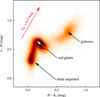 |
Fig. 1. Color distribution of stars with accurate photometry (photometric error below 0.1 mag in both colors). The various clumps have a simple direct interpretation, as indicated by the black arrows. The red arrow indicates the shift operated by a 0.5 mag K-band extinction. |
When a uniform extinction is present, the color distribution of stars is (to a first approximation, see below Sect. 2.6) shifted along the reddening vector. This suggests that we can infer the extinction that affects each object by tracing the observed colors of each object back along the reddening vector and considering the amplitudes (i.e. the values) of the iPDF along this line. These can be directly interpreted as an extinction probability distribution for the star. The same method was essentially also used by Meingast et al. (2017) in the PNICER technique.
In reality, this simple scheme has some problems that need to be solved before it can be applied in a rigorous way to real data:
-
any background object will likely have photometric errors that will affect the observed colors and that need to be taken into account;
-
some objects will also have missing bands, a fact that clearly needs to be taken into account;
-
the same two issues mentioned above (photometric errors and missing bands) will also affect the objects observed in the control field, and this will affect our capability of inferring the iPDF;
-
the population of observed background objects differs from the control field population because of the effects of extinction itself (essentially, we will miss the faintest objects).
In the following subsections we consider all these problems in detail.
2.1. Intrinsic star color distribution (iPDF)
We assume throughout that observations are carried out on D + 1 different magnitude bands. Not all objects need to have complete observations in all bands. Out of these D + 1 magnitudes, we can construct D independent color combinations. We generally build colors by subtracting two consecutive magnitude bands (we generalize below to situations where one or more bands are missing).
We desire to model the stars’ intrinsic color distribution, that is, the unextinguished colors of stars measured with no error. Here we assume that the distribution of intrinsic colors can be well described by a Gaussian mixed model (GMM): that is, calling c the D-dimensional vector of colors of a star, we have (1)
(1)
where pk(c) is the distribution of the kth component (k ∈ {1, …, K}) and wk is the associated weight. The weights are taken to be normalized to unity, so that (2)
(2)
Each component of the GMM is modeled as a multivariate normal distribution with mean bk and covariance 𝒱k: (3)
(3)
The normalizing term Z(𝒱) takes the form (4)
(4)
We model the photometric error in each band using a normal distribution, and we take the magnitude errors to be independent in each band (as is usually the case). Calling m = {m1, m2, …, mD+1} the magnitude of a star, the measured magnitudes are distributed as (5)
(5)
Following what we said earlier, we call the star colors c = (c1, c2, …, cD), where ci = mi − mi+1. With this definition, the measured colors are associated with a correlated error, where the correlation matrix takes the form (6)
(6)
Hence, a measured color ĉ is distributed according to (7)
(7)
where pk(ĉ) is the distribution of the kth component over the observed colors: (8)
(8)
We note that the error matrix 𝓔 is different for each star, and therefore this distribution changes for each star.
We model situations where one or more bands are missing with the help of a (rank-deficient) projection matrix 𝒫: that is, we assume that in such cases, instead of the full color vector ĉ, we only measure a linear combination of it given by 𝒫ĉ. For example, for the simple case D = 2, if we only measure the magnitude m1 and m3, that is, if the band 2 is missing, we set (9)
(9)
so that 𝒫ĉ = ĉ1 + ĉ2 = m̂1 − m̂3. We note that 𝒫ĉ also follows a Gaussian mixture model (GMM), with means 𝒫bk and variances 𝒫(𝒱k + 𝓔)𝒫T. With the help of a suitable P matrix, we can represent all cases of missing data, as long as at least two bands are available. We assume that this is always the case (i.e. that data with a single band are discarded a priori, since they are essentially useless for color extinction measurements).
2.2. Extreme deconvolution
A critical task of XNICER is to infer the KD(D + 3)/2 − 1 parameters of the GMM of the iPDF. In principle, this could be carried out in a Bayesian framework using standard Bayesian inference, and sampling the posterior probability with techniques such as Markov chain Monte Carlo. In practice, this task is often non-trivial because the control field typically includes a large number of objects (~billions) and very many parameters.
A simpler but very effective way of solving this problem is to use a technique called extreme deconvolution (Bovy et al. 2011). This generalizes the well-known expectation-maximization technique used in the K-clustering algorithm (see, e.g. MacKay 2003) to situations where the observed data are incomplete or have errors.
The algorithm used satisfies all our requirements: it accepts noisy and incomplete data and provides a set of best-fit parameters for a GMM model. We note that when we use this technique, we are in the position of using the entire control field data, including objects with very noisy measurements, to infer the iPDF. We also note that the results provided are, as much as possible, noise-free: that is, the recovered parameters of the GMM model in principle only include the intrinsic scatter in the true colors, and not the scatter caused by their photometric errors.
We find the optimal number of components using the Bayesian information criterion (BIC, Schwarz 1978; see also Liddle 2007). In practice, however, our validation tests show that one can limit the K Gaussian components to a relatively small number (~5–10) without significant drawbacks.
Figure 2 shows an example of extreme deconvolution with K = 5 in the control field of the VISION dataset.
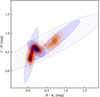 |
Fig. 2. Extreme deconvolution of the control field colors. Overimposed on the same density plot as in Fig. 1, we show ellipses corresponding to the various Gaussian distributions used in the mixture that describes this intrinsic color probability distribution. For clarity, the ellipses are 50% larger than the covariance matrices of the corresponding components. The ellipse fill color is proportional to the weight of each component. Although the model used here has five components, only four are evident: the fifth is a large ellipse that encompasses the entire figure, with a very small weight. |
2.3. Single-object extinction measurements
Extinction acts on the intrinsic star colors by shifting them: that is, an extinguished star will have its colors change as (10)
(10)
where A is the extinction (in a given band) and k is the reddening vector.
As a result, the observed distribution of an extinguished star is (11)
(11)
where as before![Mathematical equation: $$ p_k{(\widehat{\boldsymbol c})}=Z{{({\mathcal V}_k+\varepsilon)}\exp\left[-\frac12{(\widehat{\boldsymbol c}-{\boldsymbol b}_k)}^\mathrm T{({\mathcal V}_k+\varepsilon)}^{-1}{(\widehat{\boldsymbol c}-{\boldsymbol b}_k)}\right]}. $$](/articles/aa/full_html/2018/07/aa32769-18/aa32769-18-eq12.gif) (12)
(12)
We now wish to derive the distribution for the extinction, that is, p(A | ĉ), using just a single star. This can be done with Bayes’s theorem: (13)
(13)
where p(ĉ) is the marginalized likelihood or evidence: (14)
(14)
In the simplest approach, we assume a flat prior p(A) for A over the region of interest. In this way, we immediately find (15)
(15)
Here the integral in the denominator, the evidence, can be used to assess the relative goodness of fit of the GMM. This can be useful to remove potential outliers in the star distribution, that is, objects with unusual intrinsic colors (e.g. young stellar objects, YSOs) or color measurements (e.g. spurious detections). These objects will have likely incorrect extinction measurements and clearly should be excluded from the analysis.
It is convenient to analyze each term in the sum in the numerator of Eq. (15) independently. We immediately find (16)
(16)
Calling 𝒲k = 𝒱k + 𝓔 and reorganizing the various terms, we obtain (17)
(17)
where (18)
(18)
 (19)
(19)
and (20)
(20)
We note that these solutions can be written more concisely if we define a scalar product 〈· | ·〉 using the matrix  . Then we immediately have
 (21)
(21)
 (22)
(22)
and (23)
(23)
This suggests that we could perform a Cholesky decomposition of 𝒲k = ℒℒT and then apply forward substitution to calculate υ ≡ ℒ−1k and w ≡ ℒ−1(c − bk), quantities that can be used to compute all the rest: (24)
(24)
 (25)
(25)
and (26)
(26)
Finally, the integral appearing in the denominator of Eq. (15), including the component weight, is![Mathematical equation: $$ f_k\equiv w_k\;\int\;p_k{(\widehat{\boldsymbol c}-A'\boldsymbol k)}\mathrm dA'=w_kZ{({\mathcal W}_k)}\sqrt{2\pi\sigma_k^2}\exp\left[-\frac{C_k}2\right]. $$](/articles/aa/full_html/2018/07/aa32769-18/aa32769-18-eq28.gif) (27)
(27)
Therefore, the resulting distribution for p(A | ĉ) is again a mixture of Gaussian distributions and can be written directly as![Mathematical equation: $$ p{(A\;\vert\;\widehat{\boldsymbol c})}=\frac{\overset K{\underset{k=1}{\mathrm\Sigma}}\frac{f_k}{\sqrt{2\pi\sigma_k^2}}\exp{\left[-\frac{{(A-A_k)}^2}{2\sigma_k^2}\right]}}{\overset K{\underset{k=1}{\mathrm\Sigma}}f_k}. $$](/articles/aa/full_html/2018/07/aa32769-18/aa32769-18-eq29.gif) (28)
(28)
The evidence of the measurement is provided by the denominator.
We note that p(A | ĉ), as a function of A, is just a mixture of simple univariate normal distributions. In general, therefore, it will have up to K peaks, where K is the number of components used to describe the color distribution of stars.
2.4. Partial measurements
In many cases we expect to have objects that have only partial photometric measurements, that is, some missing bands. We can easily adjust the equations written above for these cases: for this purpose, we adopt a technique similar to the one used in the extreme deconvolution.
As discussed above, we can introduce for each object a possibly rank-deficient projection matrix 𝒫, and assume that instead of measuring the color vector ĉ of an object, we can only measure the quantity 𝒫ĉ. The covariance matrix associated with photometric errors of 𝒫ĉ is just 𝒫𝓔𝒫T. We therefore redefine 𝒲k as (29)
(29)
As before, we then compute the Cholesky decomposition ℒ of 𝒲k and the associated vectors υ ≡ ℒ−1𝒫k and w ≡ ℒ−1𝒫(c−bk). With these quantities, we can then compute σk, Ak, Ck, and fk as above in Eqs. (24–26).
2.5. Mixture reduction
In some cases it might be desirable to reduce the number of components of the extinction GMM: that is, one might wish to approximate the mixture with a mixture with fewer components. Often, the approximation is obtained by merging a number of components of the mixture. This procedure is usually carried out by requiring that the merged Gaussian preserves the first moments of the merged components. Using the notation of the Gaussian mixture in the color space, this requires that (30)
(30)
 (31)
(31)
and (32)
(32)
In the above equations, all sums run over the merged components {m}. Alternatively, one can perform pruning, that is, just removing some components and redistributing the weights. This, however, is generally less effective.
When applying XNICER, we typically describe the control field colors using a handful of components. The final extinction estimates for each object will have the same number of components as the control field GMM. For some applications, we might wish to have a single extinction measurement (with associated error) for each object: this is easily achieved by using the Eqs. (30–32) above and merging all components. The resulting bmerged will be the extinction value associated with the object; likewise, the resulting Vmerged will be its variance.
2.6. Number counts and extinction
The simple approach described above ignores a key point: because of extinction, the population of observed stars changes, as intrinsically faint stars will never be observed behind a dense cloud. In general, different populations of objects will suffer in different ways from extinction: galaxies are intrinsically faint, and will be the first objects to be wiped out by a cloud.
In order to describe the effects of extinction on the population of objects, we need to know the completeness function: this is just the probability for a star of magnitude m in a given band to be observed (at that band). In general, we will have a completeness function in each band considered; in the case of the VISION data considered here, we will have three functions, corresponding to the three bands J, H, and Ks.
We model each completeness function as a complementary error function erfc: (33)
(33)
In order to fit the two parameters, the 50% completeness limit mc and the width sc, we model the number counts as simple power laws. Figure 3 shows the number counts in the J, H, and Ks bands measured in the VISION control field, together with the corresponding best fits obtained for a function of the form
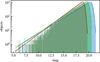 |
Fig. 3. Histograms of the number counts in the J band (blue), H band (green), and Ks band (red), together with their best-fit models in terms of exponential distributions truncated by the completeness function c(m) of Eq. (33). |
 (34)
(34)
where N0 and α are two band-dependent constants. The fact that the lines, representing the parametrization of Eq. (34), are very close to the corresponding histograms shows that the selected model for the completeness function is appropriate. This is especially true close to the completeness limit, which is the region really described by the three c functions.1 We stress, however, that any other functional form for the completeness functions can be used, as XNICER is not particularly tailored to any specific choice of c(m).
Now that we know the completeness functions, that is, the two parameters cm and sm for each band, we can simulate the presence of a cloud and artificially remove stars that cannot be observed because they are too faint. This process is carried out by computing for each star the ratio c(m + A)/c(m), where A is the extinction. This ratio gives for each star the probability to be observed when there is an extinction A. We introduce the denominator 1/c(m) in order to take into account the fact that stars in the control field have already suffered decimation by the completeness function.
Figure 4 shows the change in population of observed background stars when they are observed at increasing levels of extinction. It is evident that different components have different “survival likelihoods”: extended objects disappear almost completely when A = 2 mag, while main-sequence stars survive, although significantly decimated, up to A > 5 mag. This reflects the different number count slopes of stars and galaxies: the former are distributed in the infrared approximately as (Lombardi 2009)
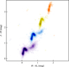 |
Fig. 4. Effects of extinction on the color distribution, from AK = 0 mag (violet) to AK = 3 mag (orange). Not only is there a global shift of the distribution, but some components disappear progressively. The various distributions are renormalized: in reality, the AK = 3 mag density is built from only the 3% brightest objects. |
 (35)
(35)
while galaxies approximately follow Hubble’s number counts (strictly valid for a static, Euclidean universe with no galaxy evolution; see, e.g. Peebles 1993): (36)
(36)
The fact that different components have different behavior behind a cloud indicates that we should use different GMMs at different extinction levels. In order to show how the population is modified, we plot in Fig. 5 the same data as in Fig. 4, but we also shift the points back along the reddening vector, so that the offset in color introduced by extinction is canceled out. This plot shows that to first order, the position and shapes of the various components are left unaffected by extinction, and that only their weights change (eventually vanishing if one component disappears).
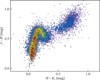 |
Fig. 5. Change in the observed background population with increasing extinction, from AK = 0 mag (violet) to AK = 3 mag (red). The shift of Fig. 4 is removed. The dominant effect is a change in relative weight of the various components, with no significant shift or change in shape. |
We therefore adopt the following strategy to take into account the effects of extinction in the population change. We build several GMMs of our objects at different extinction levels. For each object, we then use an iterative technique:
-
Initially, we assume for all objects a vanishing extinction and use the GMMs at zero extinction to infer the extinction probability distribution p(A) for each of them.
-
We then use the p(A) as a weight for the various GMMs models: that is, we build a GMM model that itself is a mixture of the GMMs models at various extinction, weighted by the corresponding p(A). Since the components of the various mixtures for different extinctions share their centers and covariances, the final GMM has the same number of components as the original GMM: this procedure does not add any further complexity to the method.
-
We repeat step 2 a few times to ensure convergence (which is achieved very quickly).
2.7. Further improvements
We can further improve our method by taking advantage of other indicators that can help us to distinguish different populations of objects. This additional step is effective if the different populations have little superposition and if they are at different places along the reddening vector.
One of the simplest possible strategies is using a reliable morphological classification to separate the objects in the color space. In our specific case, the colors of extended objects (galaxies) are very different from point-like objects (stars).
To proceed in this way, we perform two extreme deconvolutions for the different classes of objects (in a way that shares some similarities with the GNICER method of Foster et al. 2008). When computing the extinction against one object, we then use the corresponding class of the object. There are two basic ways of doing this:
-
Hard classification: every object is taken to belong to a single class. In this case, we perform separate extreme deconvolutions for each class, and use the appropriate class for each object when inferring its extinction.
-
Soft classification: each object has a set of probabilities to belong to each class. In this case, we perform separate extreme deconvolutions, but using all objects with weights corresponding to each probability; we describe the final extinction probability as a mixture of the extinction probabilities we obtain for the various classes, weighted by the object classification parameter.
We opt here for the second technique, which is more general than the first: the first technique indeed can be thought of as a particular case of the second, where the probabilities (and thus the weights) are either zero or one.
3. Comparison with different techniques
In this section we briefly compare from a purely theoretical point of view XNICER with some of the techniques that are available for extinction studies. A discussion of the various performances is carried out in the next section.
3.1. NICER
As noted above, XNICER generalizes NICER, in the sense that it decomposes the iPDF in terms of a mixture of Gaussian distributions, while NICER only uses (implicitly) a single Gaussian. In order to better understand and quantify this statement, however, it is useful to reformulate NICER from a perspective that is similar to XNICER.
NICER is implemented by considering the distribution of star colors in the control field: there, for objects with accurate photometric measurements in all bands, one measures the average color and associated covariance matrix. In the limit of negligible photometric errors, this is totally equivalent to an extreme deconvolution with a single component.
NICER then combines the control field calibration with the colors of each object to infer the extinction. The corresponding equations are virtually identical to Eqs. (19) and (18) for the extinction estimate and associated error, respectively. That is, again, NICER is a special case of a single component XNICER.
In spite of these similarities, the NICER implementation shows some significant differences if one looks in detail at its implementation. The fact that NICER does not take directly into account the photometric errors in the control field generally result in an inaccurate calibration, as we show below. This has two important consequences: extinction measurements can be (slightly) biased, and the computed errors are overestimated. We quantify both these effects for the VISION data below.
A second important difference is the lack in NICER of a correction for the population change for increasing extinction. This again results in a bias in the extinction estimated (which in general increases with extinction).
Additionally, it is worth noting that the amount of the two inaccuracies we described depends on the depth of the data used. NICER has been developed and generally used with relatively shallow data, such as are offered by the Two Micron All Sky Survey (2MASS). Additionally, the use of NICER has generally been restricted to point-like objects. Together, all this limits the biases present in NICER, since the galaxy component in the color-color plot (which is responsible for most of the population bias, the most severe one) is absent.
3.2. SCEX
Juvela & Montillaud (2016b) have developed SCEX, a series of relatively complex techniques that also aim at representing the distribution of the intrinsic colors more precisely than NICER. SCEX, in contrast to XNICER, adopts a fully non-parametric approach to describe the iPDF, which is directly inferred using kernel density estimation (KDE) techniques. Thus SCEX might be thought to be better at capturing peculiarities in the iPDF, since KDE surely allows more freedom than GMM (unless an exceedingly larger number of components is used, which generally is not the case).
In reality, precisely because of the use of KDE techniques, SCEX is completely unable to cope with photometric errors, both in the control field and in the science field. The control field color PDF is obtained from a smoothing of the star colors with a fixed kernel of 0.1 mag. However, this procedure does not lead to an estimate of the iPDF, but rather provides something that is close to a smoothed distribution of observed colors. Additionally, photometric errors are used in a very simplified way for the extinction estimate.
3.3. PNICER
PNICER uses some of the ideas of SCEX and therefore shares several similarities with XNICER. It also adopts a fully non-parametric approach to describe the iPDF, which is directly inferred using KDE techniques. Therefore, similarly to SCEX, PNICER is in principle able to better describe complex star color distributions than XNICER. Additionally, when used on single objects, instead of a simple extinction measurement with associated error, it can return a representation of the probability distribution of the extinction in terms of Gaussian mixtures. XNICER does exactly the same in a direct and natural way.
In order to understand the limitations of PNICER, it is useful to consider its implementation in detail. This algorithm works by building a representation of the control field either in magnitude or color space. Essentially, it takes all control field objects that have complete measurements on a given set of passbands and computes the density distribution using a KDE based on simple kernels with fixed bandwidth. The user is free to perform the calculations in magnitude space or color space. For a color-based PNICER, the probability that a star has a given color combination is obtained by counting how many stars in the control field have similar colors; something similar, but in magnitude space, happens for a magnitude-based PNICER. This approach necessarily introduces a number of simplifications:
-
First, similarly to SCEX, the KDE technique itself forces the code to use a single scale for the kernel. In particular, the kernel is the same not only for each star (i.e. stars with wildly different photometric errors are still used in the same way for the density estimate), but also for different color combinations. In its current implementation, the bandwidth of the kernel is chosen by taking the mean error along all color combinations.
-
PNICER, in contrast to XNICER, does not try in any way to obtain the intrinsic color (or magnitude) probability distribution iPDF: it only works on the observed distribution.
-
Additionally, when inferring the extinction of a star, PNICER ignores all star photometric errors. Simply, the observed star colors are taken as the true ones, and the error on the star extinction is just the result of the width of the control field color distribution along the reddening vector originating from the star.
-
Finally, in its current implementation, PNICER ignores all selection effects introduced by extinction; these are discussed in Sect. 2.6.
The lack of an appropriate error treatment in PNICER also implies that the errors estimated by this method are inaccurate, and indeed, our tests have shown that PNICER generally overestimates the true extinction errors by almost a factor of 2.
4. Control field analysis
As a simple test, we used the same VISION control field stars to check the performance of XNICER. For our analysis we took the control field photometric measurements and split them randomly into two sets of the same size. We then considered one of these two sets as a control field and used it to train the various algorithms, and the other as a sort of science field. In all cases, we asked the algorithms to return a single estimate for each object: this is the only possibility of NICER, and also the standard output returned by PNICER. XNICER, instead, by default provides a GMM of the inferred extinction for each object: for a more direct comparison with the other techniques, the returned GMM was converted into a single Gaussian using Eqs. (30–32).
For our tests, we considered two cases, considered separately in the following subsections:
-
Absence of any extinction, so that the “science field” is used without any modification.
-
Presence of a constant extinction value. In this case, we added to the magnitudes of all objects in the science field a suitable value (which depends on the extinction law) and simulated the effects of incompleteness.
In order to quantify the merits and weaknesses of each algorithm, it is necessary to define some quantities that summarize the bias and the average noise. Specifically, calling An and σn the extinction measurement and its associate error for the nth star, we define (37)
(37)
where Atrue is the true extinction value (set to zero in the next subsection, and to 1 mag or 2 mag in the following one). The use of the  weights in the above equations is justified by simple statistical arguments: if the {σn} are reliable estimates of the measurement errors for the {An}, the chosen weights minimize the final variance. For this reason, these weight terms are used very often when different extinction measurements need to be averaged together, as in many extinction maps of molecular clouds (see, e.g. Lombardi et al. 2010; Alves et al. 2014; Meingast et al. 2018).
In summary, b can be interpreted as the bias, and e can be interpreted as the average total error associated with each extinction measurement. In the way it is defined, e includes both the statistical error (associated with the scatter of the various An) and the systematic error (associated with the bias b).
In the following we mainly use e as a measurement of the expected total error of each method. Ideally, we would like to have e as small as possible and b as close as possible to zero. Additionally, it would be desirable that the average estimated error, 〈σn〉, be close to e, indicating that the error estimate is reliable. An inspection of the definition of e in Eq. (37) also shows that the quantity e reduces to (38)
(38)
if σn is correctly estimated and the bias b vanishes. Therefore, in the following we also consider ē to verify that the various algorithms correctly estimate their errors, so that e ≃ ē.
4.1. No extinction
In the first version of the check, we used the “science field” data without any modification. As a result, we expect to observe a vanishing extinction on average.
Figure 6 shows the extinction distributions2 obtained in the control field using XNICER, NICER, and the two PNICER variants, which we call PNICER-c (for the color-based one) and PNICER-m (for the magnitude-based one)3. For this and for the entire following analysis, we made use of the Indebetouw et al. (2005) extinction law. It is already evident from this figure that XNICER and the two PNICER versions show significantly narrower distributions than NICER. This qualitative statement is confirmed by the first column of Table 1. Moreover, PNICER-m performs better than PNICER-c, which is not immediately evident from Fig. 6: presumably, this is related to a better estimate of the weights by PNICER-m. XNICER and the two PNICER versions also have a negligible bias b.
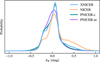 |
Fig. 6. Distribution of extinction for the control field stars, as determined using XNICER, NICER, and PNICER, both in color space (PNICER-c) and magnitude space (PNICER-m), shown using a KDE with size 0.05 mag. |
Control field results.
Figure 7 shows the distribution of noise estimates for the various methods. Interestingly, XNICER has a relatively wide distribution: in practice, it strongly distinguishes between different objects, and the noise estimate spans one order of magnitude. This distribution has a peak at very low values of σAK, which also implies that XNICER will give relatively high weights to some objects. In contrast, PNICER-c and NICER have narrow (and very similar) noise distributions, and will therefore use little weighting in the Eq. (37). PNICER-m, instead, has a large noise distribution, shifted toward relatively high values. This wide distribution is the result of an inaccurate noise estimate: as indicated in Table 1, PNICER-m predicts a noise level of ē = 0.26 mag, but the real noise is only 0.15 mag.
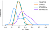 |
Fig. 7. Distribution of nominal errors for the extinction values for the control field stars, as determined using XNICER, NICER, and the two PNICER versions. |
Judging from both Fig. 7 and Table 1, PNICER-c seems to have more consistent noise properties. In reality, the algorithm shows some peculiarities in its current version, highlighted by Fig. 8: many objects are reported to have the same formal noise. This is the result of some binning operated in the PNICER-c implementation, which is necessary to implement a high speed of the algorithm. Although this does not seem to cause any severe problem for the use of the algorithm, we speculate that it might make the algorithm less efficient and might be related to the fact that PNICER-c has a slightly higher noise than PNICER-m.
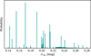 |
Fig. 8. Distribution of nominal errors PNICER-c, shown as a histogram. Many objects show the same nominal error. |
4.2. Non-vanishing extinction
We can easily simulate the effects of extinction by adding a term proportional to the reddening vector to each band. We then simulate the effects of incompleteness by statistically dropping photometric measurements for faint stars, similarly to what was done in Sect. 2.6.
Figures 9 and 10 show the results obtained for the various methods for a AK = 1mag and a AK = 2mag cloud. The corresponding b, e, and ē values are shown in Table 1. Several simple conclusions can be carried out.
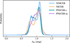 |
Fig. 9. Distribution of extinction measurements for a star of the control field when an extinction of AK = 1 mag is artificially applied. |
First, we are reassured that XNICER is able to cope well with both moderate and high extinction values: the bias is always very limited, and the error even decreases. This latter effect arises because as extinction increases, we miss the galaxy blob, and therefore the scatter in the intrinsic color of objects decreases. The formal error, ē, is also always very close to the actual error e.
Second, it is interesting to note that NICER retains much of its power even at relatively high extinction values. Admittedly, it suffers from some bias; however, it is still confined within 0.1 mag at AK = 2 mag, while its noise never increases. All this is most likely due to the simple algorithm that is used, which is able to cope well with the change of the iPDF introduced by the extinction.
Third, PNICER-c performs well as AK increases: it does not match the precision of XNICER, but is not far from it. It suffers some bias, which increases with extinction, but is still below 0.1 mag.
Instead, even a moderate extinction is able to severely affect PNICER-m. This is related to its inaccurate noise estimate: the values of ē decrease from 0.26 mag for AK = 0 mag (a value that, as we noted, is overestimated) to 0.01 mag for AK = 2 mag (a value that is clearly underestimated).
Finally, we report the result of a further test, where we apply the zero-extinction XNICER deconvolution to the extinguished control field stars. In this case, we measure a moderate bias, similar to the bias of PNICER-c (0.03 mag for AK = 1 mag and 0.07 mag for AK = 2 mag), together with a very small increase in the noise (e = 0.13 mag for AK = 2 mag and no increase at lower extinctions). These results indicate that only a small penalty is due if one desires to use a simpler algorithm and avoid the multiple fits at different extinctions.
5. Sample application: Orion A
As a first case, we applied our method to the Orion A VISION data. For this purpose, we computed the extinction against each object using NICER, PNICER-c, and XNICER. We then averaged all measurements using a standard moving-average technique, as is typically employed for extinction studies: calling An and σn the XNICER extinction and estimated noise for the nth object, we computed the extinction at the sky position x as (39)
(39)
Here xn is the angular position of the nth object, and W is a suitable weight function, taken to be normalized to unity: (40)
(40)
In this sample application, we used for W a two-dimensional Gaussian with FWHM = 2.4 arcmin. As before, we trained XNICER using a five-component Gaussian mixture, but then we merged each extinction measurement into a single value (with associated noise) by joining the various components. More sophisticated techniques for extinction spatial averaging will be considered in a follow-up paper. The result obtained, reported in Fig. 11, shows that there are no obvious problems with the algorithm.
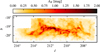 |
Fig. 11. XNICER extinction map of Orion A, using VISION data. |
Figure 12 shows the difference between the XNICER and the NICER extinction maps. This figure is dominated by relatively small fluctuations that are due to the different noise properties of the two algorithms. An investigation of the predicted noise maps shows indeed that XNICER provides overall extinction measurements in the field whose noise is a factor ~2 lower, consistent with the data shown in Table 1. The most relevant differences are observed in the densest regions, where XNICER generally provides higher extinction values (red dots in the figure): again, this is consistent with the results shown in Table 1, where we see that NICER generally underestimates the extinction for relatively high extinction values. Finally, the blue band that is observable in the top center of Fig. 12 is most likely the result of some systematic effects present in the VISION data.
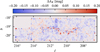 |
Fig. 12. Differences between the XNICER and the NICER extinction map of Orion A, defined as |
As an additional test, we compared object-by-object the extinction estimated using XNICER with the extinction estimated using NICER and PNICER-c; we did not use PNICER-m here because this technique, as discussed in Sect. 4, does not sample the control field for the VISION data well enough.
The results of a comparison between XNICER and PNICER-c are shown in Fig. 13. In general, we see a good match between the extinction estimates. Some of the scatter can be simply attributed to the differences in the algorithms. However, we also see a trend at high column densities: XNICER tends to return slightly higher extinction values than PNICER-c. This is consistent with our finding and with the results shown in Table 1, where we see that PNICER-c can underestimate the extinction because it ignores the effects of incompleteness.
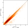 |
Fig. 13. Object-to-object comparison of the XNICER and PNICER-c extinction measurements in the Orion A field. |
We further checked this point by comparing the XNICER extinction estimates obtained with and without incompleteness correction. The result, shown in Fig. 14, confirms the trend of Fig. 13: if the incompleteness is not taken into account, we underestimate the extinction.
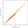 |
Fig. 14. Comparison between the XNICER extinction estimates obtained with the effects of the incompleteness (XNICER+) and without them (XNICER−). XNICER− can underestimate the extinction. |
6. Implementation
XNICER has been implemented in Python. It uses standard scientific libraries (numpy, scipy, and scikit-learn). Additionally, it relies on the extreme deconvolution algorithm4 of Bovy et al. (2011), which is available as a dynamic C library with (among others) Python wrapper. The library can take advantage of parallel processing capabilities through the OpenMP programming interface.
The extreme deconvolution of the control field data, which can be considered as a training phase in the algorithm, is a critical step and usually the most computationally intensive one. The execution time heavily depends on the number of components that are fit: however, during our tests, the training on the VISION data (comprising slightly more than 80 000 objects) has required approximately one minute for five components on a personal computer. We therefore expect that extreme deconvolutions on much larger datasets should be possible without difficulties using more powerful workstations.
The rest of the algorithm does not pose any particular computational challenge and is executed in a fraction of a second for large datasets. This is advantageous since in normal application, the science field contains many more stars than the control field where the training step is carried out.
In summary, we do not envisage any particular technical difficulty to apply XNICER to large datasets. We plan to release the full code shortly after the publication of this paper.
7. Conclusions
We have presented a new method for performing precise extinction measurements using arbitrary multi-band observations. The method, implemented in the Python language, enjoys a number of useful properties that we summarize in the following points:
-
It provides a reliable description of the intrinsic colors of stars in terms of a Gaussian mixture model. For this purpose, it makes use of the extreme deconvolution technique.
-
It is based on rigorous Bayesian statistical arguments and fully takes into account all noise properties of the control field and science field objects. Moreover, it can be applied without any difficulty to objects with partial photometric measurements (measurements only in a subset of the available bands).
-
It provides the extinction probability distribution directly for each object. This quantity is returned already decomposed in terms of a GMM. If required by the specific application, the full output can be reduced to two simple quantities: the object mean extinction, and its associated error.
-
The method has been further improved to take into account the effects of incompleteness as a consequence of an increasing extinction. Furthermore, it can also make use of additional information, such as the object morphology.
-
Our tests have shown that the method performs very well under a range of conditions and outperforms the NICER and PNICER techniques. In particular, we have shown using the Orion A VISION data that XNICER reduces the noise of extinction measurements by approximately a factor two with respect to the NICER algorithm, and that, in contrast to NICER and PNICER, it is not affected by any significant bias even at high extinctions.
Acknowledgments
We thank the anonymous referee for helping us to improve the paper significantly. We are grateful to Stefan Meingast and João Alves for their constructive comments on this work. The code at the base of this research has made use of Astropy, a community-developed core Python package for Astronomy (Astropy Collaboration et al. 2013).
Differences in the bright part of the number counts might be attributed to different measurement techniques as well as to saturation effects.
We produced this figure, as well as many of the following ones, using a KDE technique with kernel size equal to 0.05 mag.
For all tests we used the latest PNICER code available at https://github.com/smeingast/PNICER. At the time of our tests, the latest PNICER version was v0.1-beta1.
References
- Alves, J. F., Lada, C. J., & Lada, E. A. 2001, Nature, 409, 159 [NASA ADS] [CrossRef] [PubMed] [Google Scholar]
- Alves, J., Lombardi, M., & Lada, C. J. 2014, A&A, 565, A18 [NASA ADS] [CrossRef] [EDP Sciences] [Google Scholar]
- Ascenso, J., Lada, C. J., Alves, J., Román-Zúñiga, C. G., & Lombardi, M. 2013, A&A, 549, A135 [NASA ADS] [CrossRef] [EDP Sciences] [Google Scholar]
- Astropy Collaboration, Robitaille, T. P., Tollerud, E. J., et al. 2013, A&A, 558, A33 [NASA ADS] [CrossRef] [EDP Sciences] [Google Scholar]
- Bovy, J., Hogg, D. W., & Roweis, S. T. 2011, Ann. Appl. Stat., 5 [Google Scholar]
- Dobashi, K. 2011, AJ, 63, S1 [Google Scholar]
- Dobashi, K., Marshall, D. J., Shimoikura, T., & Bernard, J.-P. 2013, PASJ, 65, 31 [NASA ADS] [Google Scholar]
- Flaherty, K. M., Pipher, J. L., Megeath, S. T., et al. 2007, ApJ, 663, 1069 [CrossRef] [Google Scholar]
- Foster, J. B., Román-Zúñiga, C. G., Goodman, A. A., Lada, E. A., & Alves, J. 2008, ApJ, 674, 831 [NASA ADS] [CrossRef] [Google Scholar]
- Gaia Collaboration (Prusti, T., et al.). 2016, A&A, 595, A1 [NASA ADS] [CrossRef] [EDP Sciences] [Google Scholar]
- Goodman, A. A., Pineda, J. E., & Schnee, S. L. 2009, ApJ, 692, 91 [NASA ADS] [CrossRef] [Google Scholar]
- Indebetouw, R., Mathis, J. S., Babler, B. L., et al. 2005, ApJ, 619, 931 [NASA ADS] [CrossRef] [Google Scholar]
- Juvela, M., & Montillaud, J. 2016a, A&A, 585, A38 [NASA ADS] [CrossRef] [EDP Sciences] [Google Scholar]
- Juvela, M., & Montillaud, J. 2016b, A&A, 585, A78 [NASA ADS] [CrossRef] [EDP Sciences] [Google Scholar]
- Juvela, M., Pelkonen, V.-M., Padoan, P., & Mattila, K. 2006, A&A, 457, 877 [NASA ADS] [CrossRef] [EDP Sciences] [Google Scholar]
- Kaiser, N., Burgett, W., & Chambers, K. 2010, in, Ground-based and Airborne Telescopes III, eds. L. M. Stepp, R. Gilmozzi, & H. J. Hall, Proc. SPIE, 7733, 77330E [Google Scholar]
- Lada, C. J., Lada, E. A., Clemens, D. P., & Bally, J. 1994, ApJ, 429, 694 [NASA ADS] [CrossRef] [Google Scholar]
- Liddle, A. R. 2007, MNRAS, 377, L74 [NASA ADS] [Google Scholar]
- Lombardi, M. 2005, A&A, 438, 169 [NASA ADS] [CrossRef] [EDP Sciences] [Google Scholar]
- Lombardi, M. 2009, A&A, 493, 735 [NASA ADS] [CrossRef] [EDP Sciences] [Google Scholar]
- Lombardi, M., & Alves, J. 2001, A&A, 377, 1023 [NASA ADS] [CrossRef] [EDP Sciences] [Google Scholar]
- Lombardi, M., Alves, J., & Lada, C. J. 2006, A&A, 454, 781 [NASA ADS] [CrossRef] [EDP Sciences] [Google Scholar]
- Lombardi, M., Lada, C. J., & Alves, J. 2010, A&A, 512, A67 [NASA ADS] [CrossRef] [EDP Sciences] [Google Scholar]
- Lombardi, M., Alves, J., & Lada, C. J. 2011, A&A, 535, A16 [NASA ADS] [CrossRef] [EDP Sciences] [Google Scholar]
- Lombardi, M., Bouy, H., Alves, J., & Lada, C. J. 2014, A&A, 566, A45 [NASA ADS] [CrossRef] [EDP Sciences] [Google Scholar]
- MacKay, D. J. C. 2003, Information Theory, Inference, and Learning Algorithms (Cambridge: Cambridge University Press) [Google Scholar]
- Malinen, J., Juvela, M., Pelkonen, V.-M., & Rawlings, M. G. 2013, A&A, 558, A44 [NASA ADS] [CrossRef] [EDP Sciences] [Google Scholar]
- Meingast, S., Alves, J., Mardones, D., et al. 2016, A&A, 587, A153 [NASA ADS] [CrossRef] [EDP Sciences] [Google Scholar]
- Meingast, S., Lombardi, M., & Alves, J. 2017, A&A, 601, A137 [NASA ADS] [CrossRef] [EDP Sciences] [Google Scholar]
- Meingast, S., Alves, J., & Lombardi, M. 2018, A&A, 614, A65 [NASA ADS] [CrossRef] [EDP Sciences] [Google Scholar]
- Peebles, P. J. E. 1993, Principles of Physical Cosmology (Princeton: Princeton University Press) [Google Scholar]
- Schwarz, G. 1978, Ann. Stat., 6, 461 [NASA ADS] [CrossRef] [MathSciNet] [Google Scholar]
- Skrutskie, M. F., Cutri, R. M., Stiening, R., et al. 2006, AJ, 131, 1163 [NASA ADS] [CrossRef] [Google Scholar]
- Zari, E., Lombardi, M., Alves, J., Lada, C. J., & Bouy, H. 2016, A&A, 587, A106 [NASA ADS] [CrossRef] [EDP Sciences] [Google Scholar]
All Tables
All Figures
|
Fig. 1. Color distribution of stars with accurate photometry (photometric error below 0.1 mag in both colors). The various clumps have a simple direct interpretation, as indicated by the black arrows. The red arrow indicates the shift operated by a 0.5 mag K-band extinction. |
| In the text | |
|
Fig. 2. Extreme deconvolution of the control field colors. Overimposed on the same density plot as in Fig. 1, we show ellipses corresponding to the various Gaussian distributions used in the mixture that describes this intrinsic color probability distribution. For clarity, the ellipses are 50% larger than the covariance matrices of the corresponding components. The ellipse fill color is proportional to the weight of each component. Although the model used here has five components, only four are evident: the fifth is a large ellipse that encompasses the entire figure, with a very small weight. |
| In the text | |
|
Fig. 3. Histograms of the number counts in the J band (blue), H band (green), and Ks band (red), together with their best-fit models in terms of exponential distributions truncated by the completeness function c(m) of Eq. (33). |
| In the text | |
|
Fig. 4. Effects of extinction on the color distribution, from AK = 0 mag (violet) to AK = 3 mag (orange). Not only is there a global shift of the distribution, but some components disappear progressively. The various distributions are renormalized: in reality, the AK = 3 mag density is built from only the 3% brightest objects. |
| In the text | |
|
Fig. 5. Change in the observed background population with increasing extinction, from AK = 0 mag (violet) to AK = 3 mag (red). The shift of Fig. 4 is removed. The dominant effect is a change in relative weight of the various components, with no significant shift or change in shape. |
| In the text | |
|
Fig. 6. Distribution of extinction for the control field stars, as determined using XNICER, NICER, and PNICER, both in color space (PNICER-c) and magnitude space (PNICER-m), shown using a KDE with size 0.05 mag. |
| In the text | |
|
Fig. 7. Distribution of nominal errors for the extinction values for the control field stars, as determined using XNICER, NICER, and the two PNICER versions. |
| In the text | |
|
Fig. 8. Distribution of nominal errors PNICER-c, shown as a histogram. Many objects show the same nominal error. |
| In the text | |
|
Fig. 9. Distribution of extinction measurements for a star of the control field when an extinction of AK = 1 mag is artificially applied. |
| In the text | |
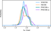 |
Fig. 10. Same as Fig. 9, but for an extinction of AK = 2 mag. |
| In the text | |
|
Fig. 11. XNICER extinction map of Orion A, using VISION data. |
| In the text | |
|
Fig. 12. Differences between the XNICER and the NICER extinction map of Orion A, defined as |
| In the text | |
|
Fig. 13. Object-to-object comparison of the XNICER and PNICER-c extinction measurements in the Orion A field. |
| In the text | |
|
Fig. 14. Comparison between the XNICER extinction estimates obtained with the effects of the incompleteness (XNICER+) and without them (XNICER−). XNICER− can underestimate the extinction. |
| In the text | |
Current usage metrics show cumulative count of Article Views (full-text article views including HTML views, PDF and ePub downloads, according to the available data) and Abstracts Views on Vision4Press platform.
Data correspond to usage on the plateform after 2015. The current usage metrics is available 48-96 hours after online publication and is updated daily on week days.
Initial download of the metrics may take a while.