| Issue |
A&A
Volume 615, July 2018
|
|
|---|---|---|
| Article Number | A168 | |
| Number of page(s) | 17 | |
| Section | Astrophysical processes | |
| DOI | https://doi.org/10.1051/0004-6361/201832731 | |
| Published online | 03 August 2018 | |
A multi-component model for observed astrophysical neutrinos
Deutsches Elektronen-Synchrotron (DESY), Platanenallee 6, 15738 Zeuthen, Germany
e-mail: This email address is being protected from spambots. You need JavaScript enabled to view it.
Received:
30
January
2018
Accepted:
8
May
2018
Abstract
Aims. We investigated the origin of observed astrophysical neutrinos.
Methods. We propose a multi-component model for the observed diffuse neutrino flux. The model includes residual atmospheric backgrounds, a Galactic contribution (e.g., from cosmic ray interactions with gas), an extragalactic contribution from pp interactions (e.g., from starburst galaxies), and a hard extragalactic contribution from photo-hadronic interactions at the highest energies (e.g., from tidal disruption events or active galactic nuclei).
Results. We demonstrate that this model can address the key problems of astrophysical neutrino data, such as the different observed spectral indices in the high-energy starting and through-going muon samples, a possible anisotropy due to Galactic events, the non-observation of point sources, and the constraint from the extragalactic diffuse gamma-ray background. Furthermore, the recently observed muon track with a reconstructed muon energy of 4.5 PeV might be interpreted as evidence for the extragalactic photo-hadronic contribution. We perform the analysis based on the observed events instead of the unfolded fluxes by computing the probability distributions for the event type and reconstructed neutrino energy. As a consequence, we give the probability of each of these astrophysical components on an event-to-event basis.
Key words: neutrinos
© ESO 2018
 Open Access article, published by EDP Sciences, under the terms of the Creative Commons Attribution License (http://creativecommons.org/licenses/by/4.0), which permits unrestricted use, distribution, and reproduction in any medium, provided the original work is properly cited.
1. Introduction
In the last few years the IceCube experiment has opened a new era in neutrino astronomy, providing the first evidence for high-energy astrophysical neutrinos (Aartsen et al. 2013). The analysis used by IceCube to claim the discovery relies on events with the interaction vertex contained in the inner detection volume, also known as high-energy starting events (HESE; Aartsen et al. 2013, 2014b, 2015a). For this analysis, a veto based on the outer detector layer has been implemented to reduce the impact of atmospheric down-going neutrinos and muons; for instance, it mainly rejects muon neutrinos accompanied by an atmospheric muon. The HESE analysis includes both muon tracks and showers (cascades) from both the southern and northern hemispheres, with slightly different sensitive energy ranges. An alternative used before the HESE discovery, and revived recently, is the detection of through-going muons (TGMs) originating from interactions of νμ from the northern hemisphere (which are free of atmospheric muon backgrounds) outside the detector (Aartsen et al. 2015b, 2016a). Similar analysis techniques are used in ANTARES (Ageron et al. 2011) and the coming KM3NeT experiment (Adrian-Martinez et al. 2016).
The origin of the observed astrophysical neutrinos remains a mystery. While the directional event distribution is isotropic at a first glance, pointing towards an extragalactic origin of most of the astrophysical neutrinos, a more detailed analysis reveals a ~ 2σ excess close to the Galactic plane when only HESE events with deposited energy above 100 TeV are considered (Aartsen et al. 2017e; see also Razzaque 2013; Ahlers & Murase 2014b; Neronov & Semikoz 2016; Palladino & Vissani 2016; Palladino et al. 2016b for recent discussions). Concerning the spectrum, the TGM dataset suggests a hard spectrum close to  , where the HESE sample is described by a much softer spectrum close to
  (Aartsen et al. 2017e). Consequently, the single power law hypothesis of the astrophysical flux has been questioned (Wang et al. 2014; Palladino et al. 2016b; Chen et al. 2015; Marinelli et al. 2016; Chianese et al. 2017; Borah et al. 2017).
Stacking searches using gamma-ray catalogs of popular candidate classes, such as gamma-ray bursts (GRBs; Aartsen et al. 2017b) and active galactic nuclei (AGN) blazars (Aartsen et al. 2017d), have revealed that the observed flux cannot be dominated by these object classes. For example, the contribution from blazars has been found to be less than about ~20% of the observed diffuse flux (Aartsen et al. 2017d; see also Palladino & Vissani 2017; Wang & Li 2016).
More generically, no point sources have been resolved to date, which indicates that most of the observed extragalactic neutrinos ought to come from abundant sources with low luminosities (Kowalski 2015; Ahlers & Halzen 2014a; Murase & Waxman 2016). If a large portion of the energy range is to be described, these neutrinos have to follow a power law with a spectral index between about  and
and  , as expected from Fermi shock acceleration for the primary cosmic rays. Such a neutrino spectrum following the primary spectrum is expected for Ap or pp interactions.
Starburst galaxies (SBGs) are ideal source candidates for this (Loeb & Waxman 2006; Tamborra et al. 2014; Chang et al. 2015; we discuss other alternatives later); however, there are two other challenges: (a) the neutrino spectrum must not be much softer than E −2 to avoid the constraint from the observed diffuse extragalactic gamma-ray background (Murase et al. 2013; Bechtol et al. 2017) and (b) cosmic-rays accelerated in SBGs are unlikely to produce neutrinos with energies much larger than PeV energies. However a muon track with a reconstructed energy of 4.5 PeV and a likely neutrino energy ≳ 10 PeV has been recently detected by IceCube (Aartsen et al. 2016a), which requires a 100 PeV primary.
Such high-energy events could come from rarer sources producing neutrinos by Aγ or pγ interactions, which typically have hard spectra which can easily peak at PeV energies and beyond (see, e.g., Winter 2013). One example, which has recently been drawing a lot of attention, are neutrinos from jetted tidal disruption events (TDEs; Wang et al. 2011; Wang & Liu 2016; Dai & Fang 2017; Senno et al. 2017; Lunardini & Winter 2017; Biehl et al. 2017a; Guépin et al. 2018), which we will use as prototypes. Compared to other sources with similar spectral properties, such as AGN blazars, we show that the TDE hypothesis can be tested by multiplet searches in the near future. In addition, a self-consistent description with ultra-high-energy cosmic rays (UHECRs) can be performed (Biehl et al. 2017a), i.e., these neutrinos may come from the sources of the cosmic rays at the highest energies. We note that in this case the primaries include nuclei heavier than protons, as indicated by recent results of the Pierre Auger collaboration (Aab et al. 2017).
Since it is clear that a single astrophysical flux component cannot address all open the questions, we propose a multi-component model to draw a self-consistent picture of the observed astrophysical neutrino flux to satisfy all of these constraints. A relevant question is the number of components really needed, which we address quantitatively. Compared to many earlier works, we start off with the information on the observed events and reconstruct the probability distribution for the reconstructed neutrino energy and interaction type (see Vincent et al. 2016; D’Amico 2018 for other examples).
The structure of the paper is as follows. In Sect. 2 we present the most recent IceCube datasets, namely the six-year HESE dataset and the eight-year TGM dataset, and we describe our procedure for obtaining the probability distribution function of the reconstructed neutrino energy (for technical details, see Appendix A). We then present in Sect. 3 our multi-component model, analyzing separately the contributions of atmospheric neutrinos, Galactic neutrinos, extragalactic pp neutrinos (such as neutrinos from SBGs), and extragalactic pγ neutrinos (such as neutrinos from TDEs or AGNs) from a theoretical point of view. We show the results of the fit in Sect. 4, where we also discuss how many components are really needed, and what we can learn in the future. An event-based assignment to the different components (probabilities) can be found in Appendix B. Finally, we summarize in Sect. 5.
2. Methods
In this section, we describe the datasets used and our energy reconstruction technique.
2.1. IceCube datasets
Here we introduce the two latest datasets provided by the IceCube collaboration after six years and eight years of data taking (Aartsen et al. 2017e), which we use for our analysis: the high-energy starting events (HESE) dataset and the TGM dataset.
2.1.1. High-energy starting events
The HESE are the events with neutrino interaction vertex contained in the detector volume; this analysis has been used by IceCube to claim the evidence of an extraterrestrial flux of high-energy neutrinos (Aartsen et al. 2013). The most recent dataset includes 2078 days (5.7 yr) of operation with 82 HESE detected: 22 muon tracks, 58 showers, and 2 events produced by a coincident pair of background muons from unrelated cosmic ray air showers that have been excluded from the analysis (Aartsen et al. 2017e). These events are characterized by a deposited energy higher than 30 TeV, and the most energetic HESE deposited an energy of 2 PeV into the detector.
The flux attributed to astrophysical neutrinos has been, to a first approximation, described by a power law spectrum and an isotropic distribution. The per-flavor flux is given by (1)
(1)
with Fℓ = 2.5 ± 0.8 and  (Aartsen et al. 2017e)1. The HESE dataset is dominated by events coming from the southern hemisphere because above several hundred TeV the absorption probability of neutrinos crossing Earth becomes greater than 50% (Aartsen et al. 2017c). In addition, we recall that the veto method of atmospheric neutrinos only works for down-going neutrinos, i.e., for neutrinos from the southern hemisphere.
The HESE are isotropically distributed when the full dataset is considered. On the other hand, when the analysis is limited to events above ~100 TeV, an anisotropy appears, with an accumulation of events close to the Galactic plane which is visible by the bare eye (see Fig. 1). The present statistical significance of this accumulation of events is about 2σ2. This slight excess of events close to the Galactic plane was already present in older IceCube datasets and has already been discussed in Neronov & Semikoz (2016), Palladino & Vissani (2016), Palladino et al. (2016b) and Pagliaroli & Villante (2017). In this work, we also take into account the possible existence of a Galactic component of high-energy neutrinos.
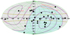 |
Fig. 1. HESE events with deposited energy above 100 TeV in Galactic coordinates (circles: showers, triangles: tracks). The purple contours represent intervals of declinations separated by 30°, whereas the brown lines denote the Galactic latitudes b = 15° and b = −15°. Taking into account that the average angular resolution of shower-like events is ~ 15°, we note an accumulation of events close to the Galactic plane, i.e., within the brown curves. |
2.1.2. Through-going muons
The IceCube collaboration has collected a sample of charged current events produced by up-going muon neutrinos from 2009 to 2017 (Aartsen et al. 2017e). The through-going muons come from muon neutrinos interacting outside the detector. Thus, in order to avoid the atmospheric muon background, the field of view must be restricted to the northern hemisphere such that atmospheric muons are absorbed on Earth.
The high-energy sample (with muon reconstructed energy above ~200 TeV) contains 36 such events; a purely atmospheric origin of them is excluded at more than 5σ. The most energetic event corresponds to a reconstructed muon energy of 4.5 PeV.
The corresponding cosmic muon neutrino and antineutrino flux was obtained with a power law fit to the data: (2)
(2)
The parameters are  and α = 2.19 ± 0.10. This analysis is sensitive mostly to muon neutrinos and antineutrinos plus a small contribution from the τ-leptons that decay into muons.
The spectral discrepancy between the HESE and TGM datasets has a significance of about 3σ and is investigated in this work.
2.2. Neutrino energy reconstruction
Here we summarize our energy reconstruction mechanism; for details, see Appendix A.
As the general ansatz we start with the list of events, sorted by topology (shower-like or track-like) and dataset (HESE or TGM); see Tables B.1–B.3. For each of these events, apart from the topology, the sky position (and its uncertainty) is known, as is the energy deposited in the detector in the form of secondary particles and, eventually, light. As initial information on the energy of each event, from here on we always use the deposited energy for shower like events and the reconstructed muon energy for TGM events. The list of events contains a residual background from atmospheric neutrinos and muons passing the veto.
The final task is to determine for each event i the reconstructed neutrino energy distribution Ci(Eν) including the probability that a shower was created from a νe, ντ or neutral current interaction, or that a track was created from a νμ or ντ induced muon. Our Monte Carlo procedure to obtain this probability distribution is described in detail in Appendix A. We note that (in terminology) we go from incident (true) neutrino energy Eν to the deposited energy Edep in the detector, which leads to a distribution for the reconstructed neutrino energy Eν, which we label in the same way as the incident energy for the sake of readability.
This reconstructed energy distribution can be used to construct binned error bars on the flux in terms of the reconstructed neutrino energy for arbitrary datasets if one deconvolves the total event rate in each bin with the effective area. This leads to results that are similar to the IceCube procedure at the highest energies (see data points in Fig. 3); however, the residual atmospheric background will show up explicitly at low energies. As another difference, we separate tracks and showers since the track sample is more affected by atmospheric backgrounds than the shower sample, which will be relevant for the construction of our multi-component model.
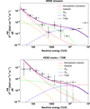 |
Fig. 2. Best-fit model (curves) and unfolded IceCube energy spectrum (points with error bars) for showers (upper panel) and tracks (lower panel) using our method described in Appendix A, where the best fit for tracks in Table 2 has been used. Black dots (and error bars) refer to HESE data and pink/light dots (and error bars) to TGM, which contains the 4.5 PeV reconstructed energy track. The energy scale refers to reconstructed neutrino energy (data) and incident energy (model). The different contributions (and the total) for the multi-component model are shown, as indicated in the plot legends. Compared to the IceCube analysis, the residual atmospheric background is shown explicitly both in data and model. |
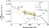 |
Fig. 3. Comparison between our multi-component model and the latest IceCube analysis including 6 yr of HESE (black points) and 8 yr of TGM (yellow band) from Aartsen et al. (2017e; neutrino flux per flavor). We find good agreement above a few hundred TeV both with HESE and TGM, whereas the two points at low energies are in tension with the model. Compared to Fig. 2, here the atmospheric backgrounds have been subtracted in both the data points and the model. |
3. Multi-component model
In this section we introduce our model, which includes (i) the atmospheric background (conventional and prompt neutrinos, atmospheric muons) since we include it in the reconstructed data points; (ii) Galactic neutrinos generated in pp collision in the Galactic disk plus Galactic neutrinos from point sources; (iii) extragalactic neutrinos from pp (or Ap) interactions, such as neutrinos from SBGs; and (iv) neutrinos from pγ (or Aγ) interactions, such as neutrinos produced in TDEs, AGNs, or GRBs. We summarize these different components in Table 1.
Summary of the main characteristics of the different components that are present in our multi-component model.
3.1. Residual atmospheric backgrounds
Atmospheric neutrinos and atmospheric muons passing the veto system produce a residual background for the high-energy neutrino detection. The conventional atmospheric (neutrino and muon) background follows the atmospheric muon spectrum ∝ E−3.7 (determined by the initial cosmic-ray spectrum modified by interactions of pions and kaons), whereas prompt neutrinos at higher energies are characterized by an E−2.7 spectrum (following the initial cosmic-ray spectrum because the secondaries decay faster than they interact). The flavor composition of atmospheric neutrinos is to a good approximation (νe : νμ : ντ) ≃ (0 : 1 : 0) in the first case, where pion decays dominate and kaon decays give a smaller but not negligible contribution. In pion decays, muon neutrinos and muons are produced. The secondary muons have no time to decay before reaching the surface of the earth; therefore, the conventional background is essentially given by νμ and v̄μ. For the prompt neutrinos, the flavor composition is given by (νe : νμ : ντ) ≃ (1 : 1 : 0) since charmed meson decays dominate here.
Atmospheric muons contribute to the background from the southern hemisphere (down-going events). We note that we do not consider the actual atmospheric fluxes, but a residual background passing the veto systems with a normalization describing observations.
The HESE track sample is much more affected by the atmospheric backgrounds than the HESE shower sample because atmospheric muons dominate this background (in the southern hemisphere) and the atmospheric electron neutrino flux, leading to showers, is suppressed compared to the muon neutrino flux (in the northern hemisphere). In order to avoid a bias on the shower sample, we assume different backgrounds for the øμ and øe fluxes in our model, reflecting the different systematics of these topologies:![Mathematical equation: $$ \frac{\mathrm d\phi_\mathrm{atmo}^{e,\mu}}{\mathrm dE_v}=\frac{10^{-18}}{\mathrm{GeV}\;\mathrm{cm}^2\;\mathrm s\;\mathrm{sr}}\left[ F_\mathrm{atm}^{e,\mu}{\left(\frac{E_v}{100\;\mathrm{TeV}}\right)}^{-3.7}+F_\mathrm{prompt}{\left(\frac{E_v}{100\;\mathrm{TeV}}\right)}^{-2.7}\right]. $$](/articles/aa/full_html/2018/07/aa32731-18/aa32731-18-eq11.gif) (3)
(3)
Here  and
and  are two free parameters (systematics) of the model, whereas we fix Fprompt = 0.66 to the present upper limit of the prompt neutrino flux per flavor (Aartsen et al. 2017e). This choice is motivated by a conservative background estimate, consistent with the total background expected for shower-like events in IceCube (Aartsen et al. 2017e). We show later that the prompt contribution does not affect our results because it is about an order of magnitude smaller than the astrophysical contributions.
We recall that the background expected by IceCube is in tension with the observations, as they expect  background tracks (see Table 3 in Palladino et al. 2017), whereas only 22 tracks have been observed (Aartsen et al. 2017e). We note that in addition the astrophysical signal contributes to the track-like events (about 20% of the astrophysical neutrinos should produce tracks, assuming pion decay as production mechanism; Palladino et al. 2015). This implies that about 40 tracks are expected instead of the 22 observed, which represents a discrepancy of about
  ; this tension between expectation and observation was already present in the older datasets (see, e.g., Table 4 in Aartsen et al. 2014b for the three-year dataset).
In our analysis, the two systematics parameters  and
and  are to be marginalized over, which means that no particular input is assumed for them. We verify that, at the end, we are able to reproduce the total background event expected by IceCube, namely
  events, reasonably well (Aartsen et al. 2017e). While this procedure does not affect our result at the highest energies or for the astrophysical components qualitatively, the obtained values for the systematics parameters can be interpreted with respect to a possible mis-identification of events and with respect to the possible origin of the discussed track discrepancy.
3.2. Galactic component
The presence of a Galactic component that could especially affect the events coming from the southern hemisphere has been already proposed in Neronov & Semikoz (2016), Palladino & Vissani (2016), Palladino et al. (2016b), Denton et al. (2017) and Marinelli et al. (2016) based on the IceCube observations. A guaranteed (diffuse) flux comes from the interactions of cosmic rays with gas; however, this contribution is typically small in models where the local cosmic ray density is assumed to be representative for the whole Milky Way (Ahlers & Murase 2014b; Joshi et al. 2014). If, however, a possible inhomogeneous cosmic ray distribution in our galaxy is taken into account, higher contributions can be obtained. In Pagliaroli et al. (2016) this flux has been calculated taking into account different cosmic ray distributions; the most optimistic case corresponds to the so-called KRAγ model (Gaggero et al. 2015), in which the spectral index of cosmic rays is a function of the distance from Galactic center, i.e., harder when close to the Galactic center and softer when far away. In this scenario the expected number of HESE in IceCube is about six contribution fro after 5.7 yr of exposure. The additional contribution from Galactic point sources is considered in Pagliaroli & Villante (2017). The expected number of events from point sources is about three with the present exposure. Therefore, the total expected number of Galactic events must not exceed nine HESE in about 6 yr of detection. These theoretical expectations are perfectly compatible with the most recent experimental limits on the Galactic flux provided by ANTARES (Albert et al. 2017) and the IceCube (Aartsen et al. 2017a).
Following these considerations, we propose a Galactic flux that is in agreement with the present knowledge. Considering that the observed flux of Galactic cosmic rays observed at Earth is E−2.7, we expect that high-energy neutrinos produced by pp interactions between Galactic cosmic rays and gas will follow the power law spectrum of the primary particles being somewhat harder from the interactions ∝ E−2.6 (Kelner et al. 2006). We assume this shape in our multi-component model. We note that in a more aggressive scenario, such as the KRAγ model, the neutrino spectrum could be harder. A harder galactic neutrino component has been analyzed in Palladino et al. (2016b). This choice would reduce the discrepancy between what is observed from the south and from the north, increasing by a small percentage the normalization of our “residual atmospheric background”. Since we are looking for a Galactic component that can emphasize the north–south spectral asymmetry, we assume a softer spectrum in our model. We note that we check the compatibility with the present constraints (from both theory and experiment) at the end of the calculations.
We use an energy cutoff in the neutrino spectrum at the corresponding knee of the cosmic rays at about 3 PeV for protons and, correspondingly, 150 TeV for neutrinos3, considering that the average energy of neutrinos from pp interaction is 5% of the primary proton energy (Kelner et al. 2006). This cutoff is compatible with recent multi-component models for cosmic rays at around the knee (Gaisser et al. 2013; see Fig. 1 in Joshi et al. 2014 for the neutrino flux), assuming that the proton component dominates the neutrino production; it is also compatible with theoretical arguments on the maximum acceleration energy of Galactic cosmic rays (Ellison et al. 1997).
Consequently, the diffuse Galactic flux of high-energy neutrinos is assumed to follow (4)
(4)
where the only free parameter is the normalization Fgal. In order to satisfy the present theoretical limits, we evaluate the expected number of events as (5)
(5)
using the average HESE effective area (Aartsen et al. 2013). This is a good choice since different intervals of terrestrial declination are covered in the inner Galaxy region, namely from −90° ≤ δ ≤ 30° (see also Fig. 1)4. We obtain from Eq. (5) that Ngal ≃ 8.4 × Fgal × T/(5.7 yr), which implies that Fgal ≲ 1.1 in order not to overshoot the nine Galactic events expected in 6 yr considering the most optimistic model, as described above. We verify whether our final result is in agreement with this constraint in the following.
Finally, we note that we have multiplied Eq. (5) with the full solid angle 4π, which does not mean that the Galactic flux is present in the whole sky. However, this choice allows for an easy comparison with the IceCube measurement, for which the average flux is usually given per steradian. In our model we take into account that the Galactic flux is present in the region of Galactic latitude |φ| ≤ 5° and of longitude |λ| ≤ 45° (inner galaxy), whereas it is not present outside. Therefore, we can write the normalization in an alternative manner for the Galactic components, as
where Ω = 4 sin |φmax| · |λmax|, with |φmax| = 5° and |λmax| = 45°.
3.3. Extragalactic pp neutrinos (Xpp)
Neutrinos are created via pp (or Ap) interactions in astrophysical environments rich in gas, which serve as target for the interactions. In this case the accelerated primaries with a non-thermal spectrum collide with thermal protons, producing about equal amounts of π+, π0, and π− leading to a neutrino spectrum adopting the spectral shape of the non-thermal primaries, which is typically a power law with a spectral index of about two.
Our prototype candidate class are SBGs, although this is not the only possible source class. A SBG is a galaxy that has an extremely high star formation rate, on the order of 10–100 M⊙ yr−1 while normal galaxies have a rate of 1–5 M⊙ yr−1 (Kewley et al. 2001). A SBG is full of young stars, which implies that supernova events are frequent, with a rate on the order of 0.03–0.3 per year; moreover, it must contain a large amount of gas available to be injected into the star-forming processes. The simultaneous presence of cosmic rays, accelerated in shock waves created by the exploding core-collapse SNe, and targets, i.e., large amounts of gas, makes SBGs promising sources of cosmic neutrinos produced by pp interactions. SBGs are mainly observed in the infrared band because the bulk of their emission (UV radiation emitted by young stars) is absorbed and re-emitted in this band.
Starburst galaxies have been proposed in several papers as sources of IceCube neutrinos (Loeb & Waxman 2006; Tamborra et al. 2014; Chang et al. 2015), although they cannot explain the entire IceCube signal (Bechtol et al. 2017; Murase & Waxman 2016). There have been many other alternatives discussed in the literature, which potentially also fit this category, such as radio galaxies (Tavecchio et al. 2018), AGN winds (Liu et al. 2018), and halo/galaxy mergers (Yuan et al. 2018).
In our model, we assume an E−2 spectrum with an energy cutoff for neutrinos at 1 PeV (Loeb & Waxman 2006): (6)
(6)
This choice of the spectral shape for SBGs is motivated by the calorimetric limit, implying that the secondary spectrum follows the primary spectrum because the interactions are the dominant process and the particle spectrum inside the SBG is not modified by energy-dependent escape processes in that energy range. The cutoff energy is motivated by the knee of the cosmic ray spectrum, which may be somewhat higher than in our galaxy because of larger magnetic fields; we note, however, that the accelerators themselves have to produce particles with high enough energies. Alternative scenarios such as acceleration in superwinds of SBGs have been discussed (e.g., Chang et al. 2015; Romero et al. 2018; Anchordoqui 2018). Our proposed spectrum is also compatible with the extragalactic diffuse gamma-ray background measured by Fermi Bechtol et al. (2017; see Murase & Waxman 2016), applied to the non-blazar contribution5.
3.4. Extragalactic pγ neutrinos (Xpγ)
Neutrinos are produced by pγ (or Aγ) interactions in astrophysical environments with high radiation densities. The accelerated primary protons (with a non-thermal spectrum) collide with photons to produce pions. In such interactions, the spectrum of the neutrinos depends on both the spectra of the primaries and the target photons.
We chose TDEs as our baseline source since we have a model available (Biehl et al. 2017a), which can describe not only the PeV neutrinos, but also the UHECRs in a self-consistent way. Other candidate classes include active galactic nuclei (see, e.g., Stecker et al. 1991; Nellen et al. 1993; Stecker 2013; Murase et al. 2014; Rodrigues et al. 2018) and low-luminosity gamma-ray bursts (see, e.g., Waxman & Bahcall 1997; Dermer & Atoyan 2003; Murase et al. 2006, 2008; Hummer et al. 2012; Zhang et al. 2018), which however require more study to draw a fully self-consistent picture. There are ways to discriminate between TDEs and other source classes, for example by neutrino point source searches, which we discuss below. We note again that the UHECR connection requires nuclei in the sources, which means that our TDE example is actually based on Aγ interactions.
Tidal disruption is the process by which a star is torn apart by the strong gravitational force of a nearby massive or supermassive black hole. About half of the star’s debris remains bound to the black hole, and is ultimately accreted. TDEs as the sources of extragalactic neutrinos have been recently very actively discussed in the literature (Wang et al. 2011; Wang & Liu 2016; Dai & Fang 2017; Senno et al. 2017; Lunardini & Winter 2017; Guépin et al. 2018; Biehl et al. 2017a). In our model we assume that the shape of the neutrino spectrum follows the best-fit spectrum of Biehl et al. (2017a), which we refer to as  , with a free normalization:
 (7)
(7)
It should be noted that the parameter FX−pγ can be directly related to the normalization G defined in Biehl et al. (2017a): (8)
(8)
Here ξA is the baryonic loading (defined as the energy injected as nuclei over the total X-ray energy in the Swift energy range 0.4–13.5 keV) and R̃(0) is the local apparent rate of jetted TDEs. The reference value chosen for R̃(0) is the rate of white dwarf–intermediate mass black hole disruptions inferred from observations, R̃(0) ~ 0.01–0.1 Gpc−3 yr−1. Thus, the result of our combined fit can be immediately interpreted in terms of the TDE baryonic loading × local apparent rate.
4. Results
In this section we present our results, including the best-fit model and the result of our energy reconstruction technique. We also demonstrate how to determine the origin of individual events at the probabilistic level.
4.1. Best-fit model
We perform a maximum likelihood analysis using a Poissonian χ2 with the different components introduced in Sect. 3 and the free parameters  , and FX − pγ. The data points for the different tested datasets are reconstructed in energy as described in Appendix A, and the theoretical rates are computed with the effective areas similar to Eq. (A.5).
Let us first use the shower (HESE) events and the track (HESE + TGM) events separately. We obtain the best-fit parameters listed in Table 2 for the spectral fit in this case. This set of parameters is in agreement with the present constraints: the obtained Galactic flux does not violate any present limit, as can be seen from Fig. 3 of Albert et al. (2017), where different experimental and theoretical limits are illustrated. It is also interesting to note that the obtained Galactic flux is consistent with the theoretical prediction of 40 yr ago reported in Stecker (1979).
For the extragalactic flux from pp interaction, we obtained a normalization that is roughly the same as that reported in Fig. 1 of Murase & Waxman (2016). Therefore, the associated flux of γ-rays, considering both contributions provided by the direct γ-ray flux and the electromagnetic cascade, is compatible with the non-blazar contribution of the diffuse gamma-ray background, i.e., 20% of the measured extragalactic diffuse γ-ray emission. Moreover, we also checked that the γ-ray flux associated with our pp neutrinos is compatible with the value reported in Fig. 5 of Tamborra et al. (2014), where the γ-ray flux was obtained starting from the infrared radiation of the SBGs.
In addition,  and
and  reproduce the total atmospheric background expected by IceCube. However, they do not reproduce the expected number of tracks and showers separately. A misidentification of tracks as showers at the level of 30–40% could reconcile the observations and the expectations. We note again that this problem related to the background is also present in the IceCube analysis itself, since in Aartsen et al. (2017e) about 40 tracks are expected (from signal, conventional atmospheric neutrino background, and atmospheric muons) instead of the 22 tracks detected.
Most importantly, we find in Table 2 an almost equal normalization for the Galactic and Xpp contributions, independent of the sample (tracks or showers used). We note that this result only reflects the spectral distribution of the observed events. Their angular distribution and the relevance of the Galactic component in the inner Galaxy will be discussed later (see Sect. 4.2 and Fig. 5).
The evidence for Xpγ > 0 depends on the sample used: whereas the best fit is zero for showers, it is similar to the TDE best fit in Biehl et al. (2017a) for tracks, which contains the 4.5 PeV reconstructed energy TGM. We use the value obtained from the tracks in the following, as we need to describe both showers and tracks. The combined fit (showers + tracks) yields instead Xpγ ≃ 0.37, which is non-vanishing but a factor of two smaller than that suggested by the track sample only. The χ2/d.o.f. are reported in Table 2 as well; a value of around one means that the model describes data very well, while at the same time it is not “over-fitting” data.
Our main result is shown in Fig. 2, where we show showers (upper panel) and tracks (lower panel) separately, including the contributions from the individual components. We use the track best fit here since it is in good agreement with the shower fit at low energy, and we expect that it is more representative for our model at high energy since the statistics is much greater above several hundred TeV than for the shower sample. We note that the reconstructed data points are consistent with the IceCube results, and that our figure contains the residual atmospheric background both in data and fluxes explicitly (see discussion below). From the figure it is clear that our model describes both tracks and showers extremely well. At low energies, there are no obvious contradictions with the residual atmospheric backgrounds. At high energies, the possible evidence for Xpγ > 0 emerges from the TGM dataset (pink), especially the 4.5 PeV track, which is likely to be generated by an incoming neutrino above 10 PeV. A possible alternative would be to extend Xpp to higher energies, but this would raise the question of whether SBG can accelerate primaries to energies significantly beyond 100 PeV.
We note again that we show shower and track events separately since they are affected by different backgrounds. Particularly the HESE track sample is more affected by the atmospheric background, since atmospheric neutrinos and atmospheric muons both contribute to the background. For this reason the HESE shower dataset is more representative of the astrophysical signal at low energies, whereas the TGM dataset is more representative of the astrophysical signal at high energies due to the larger effective area related to TGM compared to HESE.
One of the questions we need to address is how many components we actually need. We can do that at the statistical level by removing the components one by one and re-performing the fit. The atmospheric backgrounds are inevitable as they are needed to describe the spectrum below 100 TeV; this is also statistically evident. Removing the Galactic component, the quality of the spectral fit is only marginally affected. However, we have to take into account that the Galactic component also plays a role in explaining the angular distribution of HESE events above 100 TeV, and the spectral difference between HESE and TGMs. The presence of a Galactic component, mainly observed from the southern hemisphere6, helps to reduce the difference between the observations from the south and north. Our Galactic component contributes 25% to the total signal and 30–35% of the astrophysical events coming from the south.
The Xpp component provides the largest contribution to the astrophysical signal, which is about 50%. The flat E−2 spectrum is necessary to explain the middle range of energy between 100 TeV and 1 PeV. Removing this component, the quality of the combined fit goes from  , implying a 3.5σ evidence for the Xpp contribution (even in the presence of Xpγ and after re-marginalization). Moreover an extragalactic pp spectrum, generated in sources such as SBGs, can explain the lack of correlation between neutrinos and known sources of γ-rays since SBGs are rarely observed in γ rays because the photons are reprocessed inside the sources. SBGs are also compatible with the point source bounds, as they are faint enough to avoid multiplets from the same source (Kowalski 2015; Ahlers & Halzen 2014a; Murase & Waxman 2016).
The evidence for the Xpγ contribution is much weaker from the purely statistical perspective alone7. If we used the fit from the track sample, the pγ component would be responsible for about five or six events, which are the most energetic ones. Future measurements and particularly IceCube-Gen2, with a 6–8 times greater exposure (Aartsen et al. 2014d) can clarify the situation, confirming or excluding the presence of a pγ component at PeV energies. If interpreted as jetted TDE contribution, we find about 80% of the flux normalization in Biehl et al. (2017a), which can be interpreted, for example in terms of a lower baryonic loading ≃ 430 (see Eq. (8)).
Since TDEs are potentially very luminous neutrino sources, we would eventually expect several events from the same source. We compute the probability of observing at least two or three events from at least one TDE explicitly in Fig. 4 as a function of the baryonic loading, assuming that the typical TDE flux corresponds to that given in Lunardini & Winter (2017, Fig. 2, upper left panel)8. From this figure, it is evident that the probability of observing two events from one TDE is less than 50% in the current sample, and the probability for a triplet is at the percent level. We note that the limit for individual TDEs, such as Swift J1644+57 Burrows et al. (2011), can be stronger as the effective area depends on declination. However, in the future this method will be a powerful tool used to identify the origin of the Xpγ contribution and to discriminate TDEs from other classes of sources such as LL-GRBs and AGNs. Other methods include the test of a possible flavor transition at the highest energies, which is expected for TDEs (Lunardini & Winter 2017) and GRBs (e.g., Baerwald et al. 2012) due to magnetic field effects on the secondary pions, mesons, and kaons, but not for AGNs.
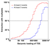 |
Fig. 4. Probability to observe multiplets of at least two events (red line) or three events (blue line) from the same TDE as a function of the baryonic loading, considering the present IceCube exposure (5.7 yr). |
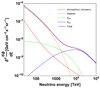 |
Fig. 5. Fluxes in the inner Galaxy, i.e., the region in Galactic coordinates |φ| ≤ 5° and |λ| ≤ 45°. The spectra are obtained using the best-fit parameters of the multi-component model. The Galactic flux is enhanced in this region compared to the averaged fluxes in Fig. 2, whereas it vanishes outside the Galaxy. |
In Fig. 3, we compare our model to the data points of the IceCube analysis in which the background has been already subtracted (Aartsen et al. 2017e). We notice a good agreement between our model and the IceCube data points in the energy range between 300 TeV and several PeV, and between our reconstructed points (see pink points in Fig. 2) and the IceCube fit of the through-going muons (yellow band in Fig. 3). On the other hand, at low energies, a certain discrepancy is present. The observation of the excess at 150 TeV by IceCube could be related to an underestimation of the background, since in their data points the background is already subtracted. The gap around 600 TeV is only present in the HESE shower dataset in our analysis, whereas it is not present in our reconstructed track sample or in the IceCube TGM analysis. Therefore, it could be simply produced by a statistical fluctuation or it could be a hint of the change of the flavor composition at very high energy, although there are not enough data to confirm the last hypothesis.
A special remark concerns the upper limit close to 7 PeV, which is in the Glashow resonance region (Glashow 1960). It is plausible that the reconstruction of this data point is strongly affected by the production mechanism. In the IceCube analysis, usually ϕνe = ϕv̄e is assumed (see, e.g., Fig. 7 in Aartsen et al. 2013). This assumption applies to pp interactions, whereas the flux of electron antineutrinos can be suppressed for the pγ production of neutrinos (Barger et al. 2014; Palladino & Vissani 2015; Palladino et al. 2016a; Biehl et al. 2017b), especially in the damped muon regime where the electron antineutrino flux at detection is strongly suppressed. A comparison to the track sample (lower panel in Fig. 2) is therefore safer here. We also checked that the number of Glashow resonant events in the most optimistic case (pp interactions) is roughly 0.5 after 5.7 yr of exposure using the best-fit parameters of the model and the approximation for the effective area from Palladino et al. (2017), which means that at present, our model is compatible with the non-observation of Glashow events. A similar estimate can be performed for double pulse events for Eν ≳ 0.5 PeV (Aartsen et al. 2016b), i.e., the detection of two separate interaction vertices for ντ. Using the effective area in Palladino et al. (2016a) and assuming that only ντ is created at the source (unrealistic, but the most conservative scenario), we expect about 0.5 double pulse events after 5.7 yr of exposure for our model. Again, our model is compatible with the non-observation of double pulses at present.
Obtained flux normalizations at the best fit for showers (HESE), tracks (HESE+TGM), and combined fit (both showers and tracks).
4.2. Event-by-event analysis
Using our multi-component model, we can compute the possible origin of each observed HESE or TGM based on their reconstructed energy and on their direction. This procedure can be sketched as follows (for details, see below):
-
Determine the distribution of the reconstructed energy of each event as described in Appendix A;
-
Determine the probability of belonging to each component of the multi-component model (best fit) according to the spectrum, performing a Monte Carlo extraction of the reconstructed energy;
-
Determine the probability of belonging to the Galactic contribution according to direction and directional resolution.
In order to include the direction of each event in our calculation, we need a function related to the compatibility of a certain direction with the Galactic plane since the Galactic flux is present in the inner Galaxy, but is absent outside, including the directional resolution of the events. We note that the Galactic flux actually dominates in the inner Galaxy region up to energies of about 2 PeV, as illustrated in Fig. 6, whereas it is absent outside this region. Since we have assumed that the Galactic flux is present in the region |φ| ≤ 5° and |λ| ≤ 45°, we define the directional probability density function such that it is one in that region and drops exponentially outside with the directional resolution,
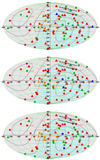 |
Fig. 6. Three different examples for the Monte Carlo assignment of the six-year HESE events to the different components in our multi-component model on an event-by-event basis (Galactic coordinates). Each color represents a component: red for atmospheric origin, orange for Galactic origin, green for Xpp, and blue for Xpγ. Circles represent showers and triangles represent tracks. The orange lines represent the region in which the Galactic component of high-energy neutrinos could be present (light orange) and the region in which a shower-like event is still compatible with Galactic origin (dark orange) within its angular resolution of about 15° (on average). |
 (9)
(9)
where G is a Gaussian function similar to Eq. (A.1) (but normalized in the range −∞ to +∞) with mean value mh and standard deviation σh, and Θ is the Heaviside step function. We use two functions for Galactic latitude and longitude, i.e., h corresponds to φ or λ; the product of the previous two functions gives the compatibility  of each event with a Galactic origin, based on its direction. We note that we have mφ = 5° and mλ = 45° by construction, whereas the standard deviations are different for showers and tracks, for which we use average values σφ = σλ ≃ 15° and σφ = σλ ≃ 1°, respectively (see, e.g., Aartsen et al. 2013). The physical meaning of this function is that an event inside the inner Galaxy is fully compatible with a Galactic origin (Cgal = 1), whereas the probability drops exponentially to Cgal = 0 going away from the inner Galaxy. To have the overall probability we have to include the information coming from the energy spectrum.
Therefore, the overall probability of belonging to a certain component is given by (10)
(10)
based on the spectrum at the reconstructed energy Eν. Since the reconstructed energy is not unique, we perform a Monte Carlo simulation (integration) to determine the average probability.
Using this procedure and integrating over Eν in Eq. (10), we can derive the probabilities that an event belongs to the different component. Since the list of events includes the atmospheric backgrounds, it should be clear now why we have carried the residual atmospheric background through the whole procedure. We give the individual probabilities that each event belongs to atmospheric background, Galactic contribution, Xpp, and Xpγ in Appendix B. We find for the HESE showers very high probabilities of belonging to the atmospheric background in most cases, whereas in eight cases the probability of belonging to the Galactic component is higher than 50%. In 25 cases, the probability of belonging to Xpp is higher than 30% (up to around 50%), whereas only two events exhibit some evidence of belonging to Xpγ (probabilities of 34 and 40%). For the HESE tracks, most events seem to belong to the atmospheric background with five exceptions with a significant probability (larger than 30%) of belonging to Xpp. The TGM sample, on the other hand, seems to be dominated by Xpp, whereas one event may be of Galactic origin and 12 events have a probability higher than 30% of belonging to Xpγ; the 4.5 PeV muon track belongs to that component with an 83% probability. The TGM sample is therefore the sample least dominated by the background and maybe best suited to study the extragalactic neutrino fluxes, whereas the Galactic contribution hides in the HESE showers. Our result is comparable with that obtained in Feyereisen et al. (2017a, 2017b), where the signal is mostly attributed to neutrinos produced in pp and pγ sources, identified explicitly as SBGs and Blazars in that case. In addition, they also found evidence for an unassociated E−2.7 component at low energy, which could be interpreted in terms of residual atmospheric background plus Galactic component in our model.
This result can be also pictorially represented; in Fig. 6 we show three different samples of the multi-component distribution produced with our Monte Carlo method based on the probability distribution for each event. The different colors corresponds to the different components as described in the figure caption. Moreover information on the topology of the observed events is reported since the circles represent showers and the triangles represent tracks. The inner Galaxy region is shown, as is the corresponding angular uncertainty for showers (dark orange lines). We note that the events close to the Galactic plane are likely to be associated with Galactic neutrinos in all the maps (orange), whereas the assignment to the component changes in many cases. Some of the events, however, have a high probability of being of atmospheric origin (red). The extragalactic flux is dominated by Xpp (green), but the assignment to this component can only be performed on a statistical basis. The Xpγ contribution (blue) tends to apply to the highest energetic events, about two or three events in the shown examples.
We also show in Fig. 7 the unfolded IceCube energy spectrum (points with error bars) for the three samples (HESE showers, HESE tracks, and TGM) separated into the different components. Here the method described in Appendix A is used, separating the event rate contributions of the different components. We note that the data points and error bars are obtained using the probability Eq. (10), which means that they depend on our model, whereas the points reported in Fig. 2 are model independent. We can use the figure to see what datasets at what energies describe the different components. For example, we can see that the residual atmospheric backgrounds are well determined at low energies from the HESE data. The HESE showers constrain the Galactic contribution well around 100 TeV, whereas the Xpp contribution is equally well contributed to by HESE showers, tracks, and TGMs. The evidence for Xpγ is mostly driven by the TGM sample.
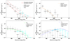 |
Fig. 7. Best-fit model (curves, for track best-fit in Table 2) and unfolded IceCube energy spectrum (points with error bars) for HESE showers, HESE tracks, and TGMs using the method described in Appendix A. Here the data points and error bars are shown for the individual contributions given by the different components, i.e., they depend on the event splitting as given by the fit of the multi-component model. |
Our analysis is only useful on a statistical basis, but it can be easily extended to future datasets. It allows us to use the information about an individual component if a theoretical model for one source class is studied. There are some limitations of our method. First of all, we do not take into account individual directional uncertainties for the events, which could be used to make the analysis more precise. In order to obtain the uncertainties in Galactic coordinates, a Monte Carlo extraction would be required since the direction and the uncertainties of each event are given in equatorial coordinates and the transformation is not trivial. For the sake of simplicity, in Eq. (9) we use the average values of the angular resolution 1° and 15° for tracks and showers, respectively.
Second, the effective area is actually declination-dependent, whereas we use averaged effective areas. This describes the isotropic extragalactic component, and itisagood approximation for the Galactic component (as discussed in Sect. 3). For the atmospheric flux, we fit the residual atmospheric background passing the vetos and analysis chain with a free normalization independent for tracks and showers. While the effective area for individual events may exhibit a non-trivial declination-dependence, this dependence enters our free normalization as an effective average as long as the residual backgrounds roughly follow the atmospheric flux shape. The deviation between track event rate and residual background at low energies in Fig. 2, lower panel, may be an artifact of such an energy-dependent effect.
5. Summary and conclusions
In this work we have proposed a multi-component model to address the following challenges in the current data of astrophysical neutrinos:
-
The observed through-going muon spectrum, coming from the northern hemisphere, is considerably harder than the HESE sample.
-
The HESE dataset exhibits an anisotropy if only events above 100 TeV are considered, indicating a correlation with the Galactic plane.
-
No correlations with known sources have been observed; no point sources have been identified.
-
The limit from the observed extragalactic gamma-ray background must be obeyed.
-
The recent observation of a muon track with 4.5 PeV reconstructed muon energy requires a primary energy ≳100 PeV.
We have started from the event topology and deposited energy, and we have computed the probability distribution in terms of event type and reconstructed neutrino energy event by event. Consequently, we have reproduced the reconstructed energy distributions by IceCube very well. In comparison to the IceCube publications, we have included the residual atmospheric background explicitly because we have (at the end) listed the probability for each individual event to belong to each of these different components. Using this approach, we observe two differences compared to the IceCube reconstruction: we do not observe an excess at about 150 TeV, and the gap at about 600 TeV is only present in the shower, but not in the track samples, which points towards a statistical fluctuation (compare data points in Fig. 3 to those in Fig. 2).
Our model consists of four populations summarized in Table 1: residual atmospheric contribution (including prompt contribution) passing the vetos; Galactic contribution following the cosmic-ray flux; extragalactic flux from pp interactions (Xpp), such as starburst galaxies; and extragalactic flux from Aγ or pγ interactions (Xpγ), such as tidal disruption events or AGN blazars. We have taken the spectra shape for each of these components from plausible examples from the literature and we have fit the independent normalizations. We have demonstrated that the above challenges are solved in this model in the following way:
-
The through-going muon (TGM) sample is dominated by Xpp and Xpγ; as a consequence, the measured energy spectrum is close to
 in the energy range between 200 TeV and 10 PeV. On the other hand, the HESE dataset is more sensitive to low-energy events, which are much more affected by atmospheric backgrounds and by the Galactic component, especially for events coming from the southern hemisphere.
 -
Above 100 TeV, the atmospheric background is highly suppressed in the shower HESE dataset, whereas the Galactic component is visible and dominates over the other fluxes in the inner Galaxy region, justifying the 2σ excess close to the Galactic plane.
-
The dominant astrophysical Xpp contribution, for example from starburst galaxies, implies abundant sources of low luminosity which are consistent with current stacking or point source searches. Because of the relatively hard spectrum, the bounds from the extragalactic diffuse gamma-ray background can be easily avoided.
-
The observed 4.5 PeV track-like event, which is likely to be produced by a ~10 PeV muon neutrino, justifies Xpγ. As a baseline model we have used jetted tidal disruption events, which are compatible with the origin of UHECRs and with the PeV neutrino flux, as discussed in Biehl et al. (2017a).
Since the TDE events are rare but luminous, they can be tested by point source and multiplet limits in the future to discriminate this hypothesis from alternative scenarios such as low-luminosity AGN blazars or GRBs.
We note that the statistical evidence for Xpp is high (3.5σ, even if Xpγ is present), while for Xpγ it is not yet significant from the purely statistical perspective. The role of Xpγ could be taken over by the Xpp component if that were able to accelerate primaries to energies larger than about 100 PeV. While earlier theoretical arguments seem to disfavor this for starburst galaxies, there are recent hints for correlations among UHECRs and starburst galaxies at the observational level by the Auger experiment (Aab et al. 2018). An increase in exposure, such as by IceCube-Gen2, will help to test it: since about six or seven HESE per year are expected from Xpγ at PeV energies, the non-observation of these neutrinos would rule out Xpγ at 5σ after about 3 yr.
We conclude that a self-consistent description of the observed diffuse neutrino flux requires multiple contributions to the diffuse astrophysical neutrino flux, and we have drawn a self-consistent picture describing these contributions by their generic characteristics in terms of spectrum, sky distribution, and neutrino production mechanism. Our model solves the key challenges in current neutrino data, including multi-messenger constraints. In the future, it may be helpful to obtain neutrino constraints on the individual contributions in addition to the total spectrum to disentangle the contributions from different source classes. Our model will also help theorists draw a self-consistent picture if only one of the proposed generic contributions is considered.
Acknowledgments
We would like to thank Anatoli Fedynitch for useful discussions. This work has been supported by the European Research Council (ERC) under the European Union’s Horizon 2020 research and innovation program (Grant No. 646623).
In IceCube analyses, the equipartition of the flavors is usually assumed, which is roughly expected from high-energy neutrinos produced by pion decays after flavor mixing.
For one event (isotropic), the probability of ending up in the Galactic region is equal to sin b ≃ 0.26. Using this information, we derive the probability that a certain number of events are contained in this region, similarly to the calculation performed in Palladino & Vissani (2017). We obtain that the probability that four or more events are found in the Galactic region is 72%, whereas the probability that eight or more events are found there is only 7% (which translates into a 93% confidence level or 1.8σ for the eight events found there).
We assume an exponential energy cutoff for the proton spectrum, which approximately implies the square root of the exponential cutoff for the neutrino spectrum (Kelner et al. 2006).
We have checked that the result is only marginally affected when using the southern sky effective area instead of the all-sky area; the expected number of events is 10% higher considering an E−2.6 spectrum with the energy cutoff at 150 TeV. This is naturally expected; for a soft spectrum like this neutrinos around 100 TeV provide the largest contribution to the events. At this energy, the effective areas are almost independent of declination, whereas they are very different at higher energies where the absorption of neutrinos in Earth becomes relevant, penalizing neutrinos coming from the northern hemisphere.
Since γ-rays from π0 decays are produced together with the neutrinos from π± decays and these secondaries follow the primary spectrum for pp interactions, the observed extragalactic diffuse gamma-ray background (EGRB) constrains the maximally allowed neutrino flux. Since most of the EGRB is expected to come from AGN blazars, the constraint on the non-blazar contribution is even somewhat stronger (Bechtol et al. 2017). Our obtained SBG contribution will satisfy these limits, see Ref. Murase & Waxman (2016).
70% of the Galaxy is observed from the southern sky, whereas only 30% of it is observed from the northern hemisphere (see Fig. 2 in Palladino & Vissani 2016).
Here  goes to 5.7 using the TGM dataset, whereas it remains almost the same using both HESE and TGM, since there is a slight tension between HESE (which disfavors the pγ component) and TGM (which favors the pγ component).
Using the IceCube HESE effective areas (corresponding to the average TDE at random position), we find that the expected number of events coming from a single TDE N ≃ 0.24 × ξA /540. Using our multi component model and the present IceCube exposure, i.e., 5.7 yr for HESE, we find that about six events can be attributed to TDEs. This means that about 25 TDEs contribute to the flux. From this information, Fig. 4 can be explicitly computed following Palladino & Vissani (2017) using a Monte Carlo method.
Since we separate tracks and showers and we use the relative probabilities for the two different classes of events, this procedure also works correctly with atmospheric neutrinos.
Our function PDF corresponds to the function kf : replace Tf Vf by a δ-distribution as the deposited energy has been measured here.
References
- Aab, A., Abreu, P., Aglietta, M., et al. 2017, JCAP, 1704, 038 [NASA ADS] [CrossRef] [Google Scholar]
- Aab, A., Abreu, P., Aglietta, M., et al. 2018, ApJ, 853, L29 [Google Scholar]
- Aartsen, M. G., Abbasi, R., Abdou, Y., et al. 2013, Science, 342, 1242856 [CrossRef] [PubMed] [Google Scholar]
- Aartsen, M. G., Abbasi, R., Ackermann, M., et al. 2014a. J. Inst., 9, P03009 [Google Scholar]
- Aartsen, M. G., Ackermann, M., Adams, J., et al. 2014b, Phys. Rev. Lett., 113, 101101 [NASA ADS] [CrossRef] [Google Scholar]
- Aartsen, M. G., Ackermann, M., Adams, J., et al. 2014c, ApJ, 796, 109 [NASA ADS] [CrossRef] [Google Scholar]
- Aartsen, M. G., Ackermann, M., Adams, J., et al. 2014d, ArXiv e-prints [arXiv:1412.5106] [Google Scholar]
- Aartsen, M. G., Abraham, K., Ackermann, M., et al. 2015a, ApJ, 809, 98 [NASA ADS] [CrossRef] [Google Scholar]
- Aartsen, M. G., Abraham, K., Ackermann, M., et al. 2015b, Phys. Rev. Lett., 115, 081102 [NASA ADS] [CrossRef] [PubMed] [Google Scholar]
- Aartsen, M. G., Abraham, K., Ackermann, M., et al. 2016a, ApJ, 833, 3 [Google Scholar]
- Aartsen, M. G., Abraham, K., Ackermann, M., et al. 2016b, Phys. Rev. D, 93, 022001 [NASA ADS] [CrossRef] [Google Scholar]
- Aartsen, M. G., Ackermann, M., Adams, J., et al. 2017a, ApJ, 849, 67 [NASA ADS] [CrossRef] [Google Scholar]
- Aartsen, M. G., Ackermann, M., Adams, J., et al. 2017b, ApJ, 843, 112 [NASA ADS] [CrossRef] [Google Scholar]
- Aartsen, M. G., Hill, G. C., Kyriacou, A., et al. 2017c, Nature, 551, 596 [NASA ADS] [Google Scholar]
- Aartsen, M. G., Abraham, K., Ackermann, M., et al. 2017d, ApJ, 835, 45 [NASA ADS] [CrossRef] [Google Scholar]
- Aartsen, M. G., Ackermann, M., Adams, J., et al. 2017e, ArXiv e-prints [arXiv:1710.01191] [Google Scholar]
- Adrian-Martinez, S., Ageron, M., Aharonian, F., et al. 2016, J. Phys., G43, 084001 [Google Scholar]
- Ageron, M., Aguilar, J. A., Al Samarai, I., et al. 2011, Nucl. Instrum. Meth., A656, 11 [CrossRef] [Google Scholar]
- Ahlers, M., & Halzen, F. 2014a, Phys. Rev. D, 90, 043005 [NASA ADS] [CrossRef] [Google Scholar]
- Ahlers, M., & Murase, K. 2014b, Phys. Rev. D, 90, 023010 [NASA ADS] [CrossRef] [Google Scholar]
- Albert, A., Andre, M., Anghinolfi, M., et al. 2017, Phys. Rev. D, 96, 062001 [Google Scholar]
- Anchordoqui, L. A. 2018, Phys. Rev. D, 97, 063010 [NASA ADS] [CrossRef] [Google Scholar]
- Baerwald, P., Hummer, S., & Winter, W. 2012, Astropart. Phys., 35, 508 [NASA ADS] [CrossRef] [Google Scholar]
- Barger, V., Fu, L., Learned, J. G., et al. 2014, Phys. Rev. D, 90, 121301 [NASA ADS] [CrossRef] [Google Scholar]
- Bechtol, K., Ahlers, M., Di Mauro, M., Ajello, M., & Vandenbroucke, J. 2017, ApJ, 836, 47 [NASA ADS] [CrossRef] [Google Scholar]
- Biehl, D., Boncioli, D., Lunardini, C., & Winter, W. 2017a, ArXiv e-prints [arXiv:1711.03555] [Google Scholar]
- Biehl, D., Fedynitch, A., Palladino, A., Weiler, T. J., & Winter, W. 2017b, JCAP, 1701, 033 [NASA ADS] [CrossRef] [Google Scholar]
- Borah, D., Dasgupta, A., Dey, U. K., Patra, S., & Tomar, G. 2017, J. High Energy Phys., 09, 005 [NASA ADS] [CrossRef] [Google Scholar]
- Burrows, D. N., Kennea, J. A., Ghisellini, G., et al. 2011, Nature, 476, 421 [NASA ADS] [CrossRef] [PubMed] [Google Scholar]
- Chang, X.-C., Liu, R.-Y., & Wang, X.-Y. 2015, ApJ, 805, 95 [NASA ADS] [CrossRef] [Google Scholar]
- Chen, C.-Y., Bhupal Dev, P. S., & Soni, A. 2015, Phys. Rev. D, 92, 073001 [NASA ADS] [CrossRef] [Google Scholar]
- Chianese, M., Mele, R., Miele, G., Migliozzi, P., & Morisi, S. 2017, ApJ, 851, 36 [NASA ADS] [CrossRef] [Google Scholar]
- Dai, L., & Fang, K. 2017, MNRAS, 469, 1354 [NASA ADS] [CrossRef] [Google Scholar]
- D’Amico, G. 2018, Astropart. Phys., 101, 8 [NASA ADS] [CrossRef] [Google Scholar]
- Denton, P. B., Marfatia, D., & Weiler, T. J. 2017, JCAP, 1708, 033 [NASA ADS] [CrossRef] [Google Scholar]
- Dermer, C. D., & Atoyan, A. 2003, Phys. Rev. Lett., 91, 071102 [NASA ADS] [CrossRef] [Google Scholar]
- Ellison, D. C., Drury, L. O. C., & Meyer, J. P. 1997, ApJ, 487, 197 [NASA ADS] [CrossRef] [Google Scholar]
- Feyereisen, M. R., Gaggero, D., & Ando, S. 2017a, Phys. Rev. D, 97, 103017 [NASA ADS] [CrossRef] [Google Scholar]
- Feyereisen, M. R., Tamborra, I., & Ando, S. 2017b, JCAP, 1703, 057 [NASA ADS] [CrossRef] [Google Scholar]
- Gaggero, D., Grasso, D., Marinelli, A., Urbano, A., & Valli, M. 2015, ApJ, 815, L25 [Google Scholar]
- Gaisser, T. K., Stanev, T., & Tilav, S. 2013, Front. Phys., 8, 748 [NASA ADS] [CrossRef] [Google Scholar]
- Gandhi, R., Quigg, C., Reno, M. H., & Sarcevic, I. 1998, Phys. Rev. D, 58, 093009 [NASA ADS] [CrossRef] [Google Scholar]
- Glashow, S. L. 1960, Phys. Rev., 118, 316 [NASA ADS] [CrossRef] [Google Scholar]
- Guépin, C., Kotera, K., Barausse, E., Fang, K., & Murase, K. 2018, A&A, accepted DOI: 10.1051/0004-6361/201732392 [EDP Sciences] [Google Scholar]
- Huber, P., Lindner, M., & Winter, W. 2005, Comput. Phys. Commun., 167, 195 [NASA ADS] [CrossRef] [Google Scholar]
- Hummer, S., Baerwald, P., & Winter, W. 2012, Phys. Rev. Lett., 108, 231101 [NASA ADS] [CrossRef] [PubMed] [Google Scholar]
- Joshi, J. C., Winter, W., & Gupta, N. 2014, MNRAS, 439, 3414; Erratum: 446, 892 [NASA ADS] [CrossRef] [Google Scholar]
- Kelner, S. R., Aharonian, F. A., & Bugayov, V. V. 2006, Phys. Rev. D, 74, 034018; Erratum: 2009, 79, 039901 [NASA ADS] [CrossRef] [Google Scholar]
- Kewley, L. J., Dopita, M. A., Sutherland, R. S., Heisler, C. A., & Trevena, J. 2001, ApJ, 556, 121 [Google Scholar]
- Kowalski, M. 2015, J. Phys. Conf. Ser., 632, 012039 [CrossRef] [Google Scholar]
- Liu, R.-Y., Murase, K., Inoue, S., Ge, C., & Wang, X.-Y. 2018, ApJ, 858, 9 [NASA ADS] [CrossRef] [Google Scholar]
- Loeb, A., & Waxman, E. 2006, JCAP, 0605, 003 [Google Scholar]
- Lunardini, C., & Winter, W. 2017, Phys. Rev. D, 95, 123001 [NASA ADS] [CrossRef] [Google Scholar]
- Marinelli, A., Gaggero, D., Grasso, D., Urbano, A., & Valli, M. 2016, EPJ Web Conf., 116, 04009 [CrossRef] [Google Scholar]
- Murase, K., & Waxman, E. 2016, Phys. Rev. D, 94, 103006 [NASA ADS] [CrossRef] [Google Scholar]
- Murase, K., Ioka, K., Nagataki, S., & Nakamura, T. 2006, ApJ, 651, L5 [NASA ADS] [CrossRef] [Google Scholar]
- Murase, K., Ioka, K., Nagataki, S., & Nakamura, T. 2008, Phys. Rev. D, 78, 023005 [CrossRef] [Google Scholar]
- Murase, K., Ahlers, M., & Lacki, B. C. 2013, Phys. Rev. D, 88, 121301 [NASA ADS] [CrossRef] [Google Scholar]
- Murase, K., Inoue, Y., & Dermer, C. D. 2014, Phys. Rev. D, 90, 023007 [NASA ADS] [CrossRef] [Google Scholar]
- Nellen, L., Mannheim, K., & Biermann, P. L. 1993, Phys. Rev. D, 47, 5270 [NASA ADS] [CrossRef] [Google Scholar]
- Neronov, A., & Semikoz, D. V. 2016, Astropart. Phys., 75, 60 [NASA ADS] [CrossRef] [Google Scholar]
- Pagliaroli, G., & Villante, F. L. 2017, ArXiv e-prints [arXiv:1710.01040] [Google Scholar]
- Pagliaroli, G., Evoli, C., & Villante, F. L. 2016, JCAP, 1611, 004 [NASA ADS] [CrossRef] [Google Scholar]
- Palladino, A., & Vissani, F. 2015, Eur. Phys. J. C, 75, 433 [NASA ADS] [CrossRef] [EDP Sciences] [Google Scholar]
- Palladino, A., & Vissani, F. 2016, ApJ, 826, 185 [NASA ADS] [CrossRef] [Google Scholar]
- Palladino, A., & Vissani, F. 2017, A&A, 604, A18 [NASA ADS] [CrossRef] [EDP Sciences] [Google Scholar]
- Palladino, A., Pagliaroli, G., Villante, F. L., & Vissani, F. 2015, Phys. Rev. Lett., 114, 171101 [NASA ADS] [CrossRef] [PubMed] [Google Scholar]
- Palladino, A., Pagliaroli, G., Villante, F. L., & Vissani, F. 2016a, Eur. Phys. J. C, 76, 52 [NASA ADS] [CrossRef] [EDP Sciences] [Google Scholar]
- Palladino, A., Spurio, M., & Vissani, F. 2016b, JCAP, 1612, 045 [NASA ADS] [CrossRef] [Google Scholar]
- Palladino, A., Mascaretti, C., & Vissani, F. 2017, Eur. Phys. J. C, 77, 684 [CrossRef] [EDP Sciences] [Google Scholar]
- Razzaque, S. 2013, Phys. Rev. D, 88, 081302 [NASA ADS] [CrossRef] [Google Scholar]
- Rodrigues, X., Fedynitch, A., Gao, S., Boncioli, D., & Winter, W. 2018, ApJ, 854, 54 [NASA ADS] [CrossRef] [Google Scholar]
- Romero, G. E., Müller, A. L., & Roth, M. 2018, A&A, in press, DOI: 10.1051/0004-6361/201832666 [EDP Sciences] [Google Scholar]
- Senno, N., Murase, K., & Meszaros, P. 2017, ApJ, 838, 3 [NASA ADS] [CrossRef] [Google Scholar]
- Stecker, F. W. 1979, ApJ, 228, 919 [NASA ADS] [CrossRef] [Google Scholar]
- Stecker, F. W. 2013, Phys. Rev. D, 88, 047301 [NASA ADS] [CrossRef] [Google Scholar]
- Stecker, F. W., Done, C., Salamon, M. H., & Sommers, P. 1991, Phys. Rev. Lett., 66, 2697 [NASA ADS] [CrossRef] [PubMed] [Google Scholar]
- Tamborra, I., Ando, S., & Murase, K. 2014, JCAP, 1409, 043 [NASA ADS] [CrossRef] [Google Scholar]
- Tavecchio, F., Righi, C., Capetti, A., Grandi, P., & Ghisellini, G. 2018, MNRAS, 475, 5529 [NASA ADS] [CrossRef] [Google Scholar]
- Vincent, A. C., Palomares-Ruiz, S., & Mena, O. 2016, Phys. Rev. D, 94, 023009 [NASA ADS] [CrossRef] [Google Scholar]
- Vissani, F., Pagliaroli, G., & Villante, F. L. 2013, JCAP, 1309, 017 [NASA ADS] [CrossRef] [Google Scholar]
- Wang, B. & Li, Z. 2016, Sci. China Phys. Mech. Astron., 59, 619502 [CrossRef] [Google Scholar]
- Wang, X.-Y., & Liu, R.-Y. 2016, Phys. Rev. D, 93, 083005 [NASA ADS] [CrossRef] [Google Scholar]
- Wang, X.-Y., Liu, R.-Y., Dai, Z.-G., & Cheng, K. S. 2011, Phys. Rev. D, 84, 081301 [NASA ADS] [CrossRef] [Google Scholar]
- Wang, B., Zhao, X.-H., & Li, Z. 2014, JCAP, 1411, 028 [NASA ADS] [CrossRef] [Google Scholar]
- Waxman, E., & Bahcall, J. N. 1997, Phys. Rev. Lett., 78, 2292 [NASA ADS] [CrossRef] [Google Scholar]
- Winter, W. 2013, Phys. Rev. D, 88, 083007 [NASA ADS] [CrossRef] [Google Scholar]
- Yuan, C., Meszaros, P., Murase, K., & Jeong, D. 2018, ApJ, 857, 50 [NASA ADS] [CrossRef] [Google Scholar]
- Zhang, B. T., Murase, K., Kimura, S. S., Horiuchi, S., & Mészáros, P. 2018, Phys. Rev. D, 97, 083010 [NASA ADS] [CrossRef] [Google Scholar]
Appendix A: Methods (details)
In this appendix, we describe how we go from the deposited energy per event and the event topology to the reconstructed neutrino spectrum.
A.1. Description of the interactions
Here we define the probability density functions the connect the incident neutrino energy with the deposited energy.
νe charged current (CC) interactions. If electron neutrinos (antineutrinos) interact via a charge current interaction, almost all of the energy is deposited into the detector as an electromagnetic shower. Assuming that the fraction x ≡ Edep/Eν of the incident neutrino energy Eν is deposited in the detector, i.e., the deposited energy Edep = x Eν with 0 ≤ x ≤ 1, we define a probability distribution function  proportional to a Gaussian
 (A.1)
(A.1)
with the normalization (A.2)
(A.2)
For νe CC interactions, we use me,CC = 0.95, implying that most of the energy is deposited in the detector, and σe,CC = 0.06 (see Table 1 and Fig. 1 in Aartsen et al. 2014a). Our assumption can be compared to the IceCube results comparing the left panel of Fig. A.1 with the left panel of Fig. 1 in Aartsen et al. (2014a).
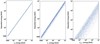 |
Fig. A.1. Relations between incident neutrino energy and deposited energy for νe and ντ CC interactions (left and middle panels) and for NC interactions (right panel). |
The probability that a neutrino is a νμ and produces a track-like event is given by
evaluated at the incident neutrino energy, where σ̂ is the cross section. The ratio σ̂CC/(σ̂CC + σ̂NC is to a good approximation constant in the energy range between 100 TeV and 10 PeV, i.e., our range of interest, and it is equal to 0.71 (Gandhi et al. 2017). Moreover we assume the equipartition of flavors in order to simplify the calculation, which leads to  9.
9.
ντ charged current (CC) interactions. If tau neutrinos (antineutrinos) interact via charged currents, a fraction of energy is carried away by neutrinos generated by τ decays which is not detectable. Considering the various channels in which a τ can decay, the average quantity of energy fraction detectable is about 80% (Vissani et al. 2013). We also use a Gaussian (see Eq. (A.1)) with mτ,CC = 1 and στ,CC = 0.25 in order to reproduce the average value of the transferred energy. Therefore, the uncertainty is larger here than for νe CC interactions (see middle panel of Fig. A.1).
Moreover ντ can produce muons with a branching ratio of B.R.(τ → μ) = 17.4%. This contribution has to be subtracted, since we only discuss shower-like events in this section. The probability that a neutrino is a ντ and interacts via charged currents producing a shower-like event is given by
which is 
Neutral current (NC) interactions. For NC interactions, which are not sensitive to flavor, a large fraction of the incoming neutrino energy is not visible because it is carried away by outgoing neutrinos. The average fraction of deposited energy is 25%, but large fluctuation are expected in this case (see Fig. 1, right panel, in Aartsen et al. 2014a). We therefore use mNC = 0 (events that deposit a small fraction of energy are favored) and standard deviation σNC = 0.3 in Eq. (A.1). This choice reproduces the average fraction of deposited energy, and it also describes to a good approximation the right panel of Fig. 1 in Aartsen et al. (2014a; cf. the right panel of Fig. A.1).
The probability that a neutrino interacts via neutral currents is given by
Track-like events: νμ. Track-like events are generated by νμ that interact via CC interaction and produce a muon, which is visible as track in the detector. For track-like events the information on the incoming neutrino energy is very uncertain and the deposited energy only represents a lower limit to the incoming neutrino energy (the track often originates outside the detector). As for NC interactions the deposited energy is usually a small fraction of the incoming neutrino energy; therefore, we use the same probability density function used for NC interaction, i.e.,  . We have checked that this approximation reproduces the measured through-going muon spectrum to a good approximation, as can be seen by comparing the pink points in Fig. 2 to the yellow band in Fig. 3.
The probability that a neutrino is a νμ and produces a track-like event is given by
Track-like events: νμ. Track-like events can be generated,
in smaller number, by muons created in the νμ CC interactions. The probability that a neutrino is a νμ which interacts via CC interaction and produces a track-like event is given by
We recall that here the muon is generated by tau decay,
which means that the muon takes about 1/3 of the ντ energy. We therefore use  .
.
A.2. From deposited to reconstructed energy
We now construct the probability density function Rℓ(Edep, Eν) (differential in Eν) of the reconstructed neutrino energy for a given deposited energy and event type ℓ. We note that for the sake of simplicity we use the symbol Eν simultaneously for the incident (true) and reconstructed neutrino energies.
Compared to the PDFs in the previous section, the function Rℓ will depend on the spectral shape. We assume an E−2 flux for the neutrino spectrum by default, but we discuss the consequences of different assumptions below. Because the cross section of neutrino-nucleons interaction scales  in the energy range between 100 TeV and 10 PeV (Gandhi et al. 2017), the function Rℓ is given by
 (A.3)
(A.3)
where the last factor is the product between spectrum and cross section energy dependencies. Here ℓ denotes one of the process previously described, namely showers given by νe CC, ντ CC, or NC interactions and tracks given by νμ CC and ντ CC interactions. The factor  comes from the change of variables from x to Eν in the normalization Eq. (A.2). In order to derive this formula, see also Sect. 2 of Huber et al. (2005)10.
The probability that an event with a certain deposited energy has been generated by a specific process becomes (A.4)
(A.4)
We have checked that these probabilities, to a very good approximation, do not depend upon the deposited energy. The probability that a shower-like event has been produced by νe CC, ντ CC, and NC interactions is 55, 35, and 10%, respectively. The probability that a track-like event has been produced by νμ CC or ντ CC interactions is 96 and 4%, respectively. We note that P̃ℓ includes the spectral redistribution of events, as compared to Pℓ, and that we have pulled out Pℓ from the integrals because they hardly depend on energy. For example,  is smaller than
  (compared to the other charged current showers) because a NC shower with a certain deposited energy tends to come from a higher energy than a CC shower where the flux is lower.
A.3. Monte Carlo simulation and deconvolved neutrino flux
Starting from the list of events with event topology (track-like or shower-like) and Edep, we construct the probability distribution for the deposited energy Ci(Eν) for the ith event as follows:
-
We determine a process that has generated the observed event from the probability P̃ℓ in Eq. (A.4).
-
We extract an energy associated with the process according to the distribution Rℓ(E dep, Eν) in Eq. (A.3).
-
We repeat this procedure 104 times to obtain the reconstructed energy distribution Ci(Eν) for this event.
We show in Fig. A.2 the distribution of the reconstructed (neutrino) energy for a shower with deposited energy of 1 PeV (left panel) and a track with reconstructed energy of 4.5 PeV (right panel), i.e., the most energetic event observed by IceCube up to now. The reconstructed energy of a shower-like event is close to the deposited energy and there is a small uncertainty, whereas the reconstructed energy of a track-like event is two to three times larger than the deposited one, with a much bigger uncertainty. We have checked that both our probability distribution and our reconstructed energies are in very good agreement with the theoretical estimates in Tables IV and V of D’Amico (2018), which appeared during the completion of this work. The choice of a softer spectrum instead of the assumed E−2 would reduce the uncertainty on the reconstructed energy, privileging the events that deposit most of their energy. We have verified that using an E−2.5 spectrum, the uncertainty on the reconstructed energy is reduced by about 30% for shower-like events and by about 25% for the track-like events, deteriorating both the agreement with D’Amico (2018) and the TGM analysis performed by IceCube (Aartsen et al. 2015b, 2017e).
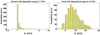 |
Fig. A.2. Distribution of the reconstructed (neutrino) energy for a shower with deposited energy of 1 PeV (left panel) and a track with reconstructed muon energy of 4.5 PeV (right panel). Here the assumption for the spectral shape is E−2. |
We can now determine the total number of events in each reconstructed energy bin j covering the energy interval [Ej, Ej+1], where the choice of the binning is arbitrary. The distribution function for all events of one topology is given by
where i runs over all events from a dataset, and the number of events assigned to the jth bin is
We assume that the uncertainty on  is
is  when Nj is large; when N is small, namely smaller than one, we set a 90% confidence level (C.L.) limit to the expected number of
  using Poissonian statistics.
Thanks to the effective areas (HESE Aartsen et al. 2013 and through-going muons Aartsen et al. 2014c) it is possible to convert the  into the expected flux in each energy interval, using the formula for shower-like HESE
 (A.5)
(A.5)
and the formula for track-like HESE or through-going muons (they differ for the effective area  )
) (A.6)
(A.6)
where
is the middle point on a log-scale, and η = 0.8 represents the fraction of the νμ effective area that is connected to track-like events (see Palladino et al. 2015). The effective areas are taken from Aartsen et al. (2013) for HESE and from Aartsen et al. (2014c) for TGM.
The reconstructed data points are shown in Fig. 2. Here the uncertainties on the flux are proportional to the uncertainties on  , as described above, whereas the uncertainties on the energy axis cover the interval between Ej and Ej+1.
In the previous calculation we assume an E−2 spectrum in each energy interval between Ej and Ej+1. This approximation is not accurate when we analyze low energies (especially for track-like events), where the atmospheric neutrino spectrum E−3.7 dominates. A possible solution is to choose small energy intervals to reduce this effect. With our assumption the background related to øμ might be underestimated in the data points at very low energies.
Appendix B: Tables of the probabilities
In this appendix we list the event-to-event probability for each IceCube event for our multi-component model. The probabilities have been obtained using Eq. (10); see main text. We show three different tables for HESE showers (Table B.1), HESE tracks (Table B.2) and TGMs (Table B.3).
HESE showers.
HESE tracks.
Through-going muons.
All Tables
Summary of the main characteristics of the different components that are present in our multi-component model.
Obtained flux normalizations at the best fit for showers (HESE), tracks (HESE+TGM), and combined fit (both showers and tracks).
All Figures
|
Fig. 1. HESE events with deposited energy above 100 TeV in Galactic coordinates (circles: showers, triangles: tracks). The purple contours represent intervals of declinations separated by 30°, whereas the brown lines denote the Galactic latitudes b = 15° and b = −15°. Taking into account that the average angular resolution of shower-like events is ~ 15°, we note an accumulation of events close to the Galactic plane, i.e., within the brown curves. |
| In the text | |
|
Fig. 2. Best-fit model (curves) and unfolded IceCube energy spectrum (points with error bars) for showers (upper panel) and tracks (lower panel) using our method described in Appendix A, where the best fit for tracks in Table 2 has been used. Black dots (and error bars) refer to HESE data and pink/light dots (and error bars) to TGM, which contains the 4.5 PeV reconstructed energy track. The energy scale refers to reconstructed neutrino energy (data) and incident energy (model). The different contributions (and the total) for the multi-component model are shown, as indicated in the plot legends. Compared to the IceCube analysis, the residual atmospheric background is shown explicitly both in data and model. |
| In the text | |
|
Fig. 3. Comparison between our multi-component model and the latest IceCube analysis including 6 yr of HESE (black points) and 8 yr of TGM (yellow band) from Aartsen et al. (2017e; neutrino flux per flavor). We find good agreement above a few hundred TeV both with HESE and TGM, whereas the two points at low energies are in tension with the model. Compared to Fig. 2, here the atmospheric backgrounds have been subtracted in both the data points and the model. |
| In the text | |
|
Fig. 4. Probability to observe multiplets of at least two events (red line) or three events (blue line) from the same TDE as a function of the baryonic loading, considering the present IceCube exposure (5.7 yr). |
| In the text | |
|
Fig. 5. Fluxes in the inner Galaxy, i.e., the region in Galactic coordinates |φ| ≤ 5° and |λ| ≤ 45°. The spectra are obtained using the best-fit parameters of the multi-component model. The Galactic flux is enhanced in this region compared to the averaged fluxes in Fig. 2, whereas it vanishes outside the Galaxy. |
| In the text | |
|
Fig. 6. Three different examples for the Monte Carlo assignment of the six-year HESE events to the different components in our multi-component model on an event-by-event basis (Galactic coordinates). Each color represents a component: red for atmospheric origin, orange for Galactic origin, green for Xpp, and blue for Xpγ. Circles represent showers and triangles represent tracks. The orange lines represent the region in which the Galactic component of high-energy neutrinos could be present (light orange) and the region in which a shower-like event is still compatible with Galactic origin (dark orange) within its angular resolution of about 15° (on average). |
| In the text | |
|
Fig. 7. Best-fit model (curves, for track best-fit in Table 2) and unfolded IceCube energy spectrum (points with error bars) for HESE showers, HESE tracks, and TGMs using the method described in Appendix A. Here the data points and error bars are shown for the individual contributions given by the different components, i.e., they depend on the event splitting as given by the fit of the multi-component model. |
| In the text | |
|
Fig. A.1. Relations between incident neutrino energy and deposited energy for νe and ντ CC interactions (left and middle panels) and for NC interactions (right panel). |
| In the text | |
|
Fig. A.2. Distribution of the reconstructed (neutrino) energy for a shower with deposited energy of 1 PeV (left panel) and a track with reconstructed muon energy of 4.5 PeV (right panel). Here the assumption for the spectral shape is E−2. |
| In the text | |
Current usage metrics show cumulative count of Article Views (full-text article views including HTML views, PDF and ePub downloads, according to the available data) and Abstracts Views on Vision4Press platform.
Data correspond to usage on the plateform after 2015. The current usage metrics is available 48-96 hours after online publication and is updated daily on week days.
Initial download of the metrics may take a while.