| Issue |
A&A
Volume 615, July 2018
|
|
|---|---|---|
| Article Number | A123 | |
| Number of page(s) | 19 | |
| Section | Extragalactic astronomy | |
| DOI | https://doi.org/10.1051/0004-6361/201732039 | |
| Published online | 26 July 2018 | |
Model simulation of jet precession in quasar PG 1302-102
1
Max-Planck Institüt für Radioastronomie,
Auf dem Hügel 69,
Bonn
53121,
Germany
e-mail: This email address is being protected from spambots. You need JavaScript enabled to view it.
2
National Astronomical Observatories, Chinese Academy of Sciences,
Beijing
100012,
PR China
3
Institute of Physics,
University of Szeged,
Dóm tér 9, 6720
Szeged,
Hungary
Received:
4
October
2017
Accepted:
11
January
2018
Abstract
Context. The study of periodic (or quasi-periodic) variabilities in optical and radio bands and quasi-periodic radio-jet swings are important to further our understanding of the physical processes in blazars. Among these the correlation between the periodic or quasi-periodic phenomena in radio and optical bands is particularly significant, because it can provide unique information about the relativistic jets and central engines in the nuclei of blazars.
Aims. We aim to investigate the possibility that the radio jet swing on parsec scales observed in PG 1302-102 (z = 0.278) is a quasi-periodic phenomenon and study its correlation with the periodic optical variability claimed in a recently published work, seeking evidence for a binary black hole system.
Methods. The precessing jet-nozzle model proposed in our previous works was applied to simulate the kinematics of the superluminal components. It is shown that the inner-jet kinematic features can well be explained in terms of the precessing nozzle model.
Results. Based on the model simulation (model fitting) of the inner kinematics for its six superluminal components, a precession period of ~5.1583 ± 0.5 yr is derived for the radio jet swing and the kinematics of all the six components are consistently interpreted. The similarity between the radio jet precession period and the optical period found in its optical light curve may be physically significant. Both periodic behaviors in radio and optical bands could be explained in terms of the orbital motion of a black hole binary, if the orbital plane makes large inclinations to the sky plane: the orbital motion of the primary hole produces the periodic jet swing and the orbital motion of the secondary hole produces the periodic optical variability as suggested in the literature. Thus the total mass and the mass ratio of the binary are estimated.
Conclusions. Based on this analysis, we show that PG 1302-102 might have a supermassive black hole binary existing in its nucleus and it is starting to enter its inspiral phase of merging. Gravitational radiation would start to dominate the energy-momentum loss for its orbital shrinkage.
Key words: galaxies: jets / galaxies: nuclei / quasars: individual: 1302-102 / quasars: supermassive black holes
© ESO 2018
1 Introduction
Blazars are objects characterized by extreme emission variability at all wavelengths from radio to γ-ray regimes. The strong variations in their radiation (flux and polarization) and the superluminal motion observed on VLBI-scales are largely related to the relativistic jets closely directed toward us. There is growing evidence that a number of blazars display a periodic (or quasi-periodic) behavior on timescales of years and decades. The observational evidence largely comes from two kinds of phenomena: (i) periodicities in optical and radio light curves which are correlated in some cases; (ii) periodic variations in (compact) radio cores mapped by VLBI, which include quasi-periodic undulating jet structures (swing of jet spines) and quasi-periodic wobbling of the ejection position angle of superluminal components. Many reports may be referred for several blazars, for example, BL Lac (Raiteri 2001; Stirling et al. 2003; Tateyama 2009); 3C273 (Abraham & Romero 1999; Savolainen et al. 2006; Calzadilla et al. 2015); PKS 0420-014 (Britzen et al. 2001); B0605-085 (Kudrayavtseva et al. 2011); 3C279 (Qian 2012, 2013); 3C345 (Qian et al. 1991; Steffen et al. 1995; Qian et al. 2009); 3C454.3 (Qian et al. 2007, 2014); OJ287 (Kikuchi et al. 1988; Villata et al. 1998; Tateyama & Kingham 2004; Valtonen & Wiik 2012; Valtonen & Pihajoki 2013); NRAO 150 (Agudo et al. 2007; Agudo 2009; Molina et al. 2014; Qian 2016); PG 1302-102 (Graham et al. 2015; Kun et al. 2015); B2 1308+326 (Lister et al. 2013; Qian et al. 2017; Britzen et al. 2017; hereafter BQS17). Most recently, Calzadilla et al. (2015) reported the detection of the jet precession on sub-parsec scales in the archetypal blazar 3C273 with the Event Horizon Telescope at 1.3 mm wavelength. These periodic (or quasi-periodic) phenomena are particularly important, because they can put useful constraints on the structure and kinematics (even the formation) of relativistic jets and their emission mechanisms. Precessing relativistic beams have been invoked to explain these periodic phenomena, and binary black hole systems and Lense-Thirring effect of a Kerr black hole have been applied to induce the precession of jets.
QSO PG 1302-102 has several special features in optical and radio bands. The most interesting feature is that its optical variability during the period [1995,2015] has been found (or cliamed) to be periodic with a period of 1884 ± 88 days (5.1583 ± 0.2409 yr). The observed variability amplitude is ± 0.14 mag about the avearge value of 14.78 mag (or amplitude 13.5%), having a sinusoid-like light curve (Graham et al. 2015). Thus PG 1302-102 has been suggested as a supermassive black hole binary candidate.
Hutchings et al. (1994) found that on arcsecond scales PG 1302-102 has a correlated optical and radio structures, similar to those observed in radio galaxy M87 and QSO 3C273. Jackson et al. (1992) detected a velocity shift between its narrow and broad Hβ lines, which could be the signature of a black hole binary in its center (Gaskell 1985). Graham et al. (2015) investigated its optical/NIR spectrum with broad emission lines (Hβ, Hα, Pa −β and Pa −α) and inferred its virial total mass in the range from 108.3 to 109.4 M⊙.
D’Orazio et al. (2015) found that its optical emission has a UV-bump like spectral distribution and suggested that the amplitude and the sinusoid-like shape of its optical light curve can be interpreted in terms of Doppler boost of emission from a steadily accreting black hole binary. They also argued that there are correlated variability at NUV and FUV wavelengths with amplitudes of ±30% and ±37%, respectively.This correlation between variabilities in optical and UV bands seems favorable for a physical origin rather a noise process. In this paper we shall show that the position angle swing of its radio jet is also periodic and has a precession period of 5.1583 ± 0.5 yr, similar to the optical period, thus enhancing its physical implications. If the periodic behavior in optical and radio bands is confirmed, the properties of the SMBB in QSO PG 1302-102 (e.g., total mass and mass ratio) can be tightly constrained or measured.
We explore the possibilities for unified interpretations of both radio and optical periodic behaviors under the binary black hole scenarios. The kinematic features of PG 1302-102 on parsec scales has been investigated by Kun et al. (2015). We briefly summarize the main results below.
It is a bright radio quasar with a core-jet structure on the pc-scale, but on the kpc-scale it shows a double jet structure as having a morphology like that of a wide-angle “head-tail galaxy”, indicating its galaxy moving in a cluster of galaxy (Fig. 4 in Kun et al. 2015).
During the period 1990–2012 six superluminal components (C1–C6) were observed. Their apparent velocities are in the range ~3 c – ~7 c.
The observed maximal and minimal position angles are ~ 33° (knot C6) and ~ 23° (knot C4). The average position angle of the jet is 31.6° ± 0.6° and the apparent opening angle of the (projected) jet cone is ~11° which can be regarded as the observed position angle swing.
Based on the estimate of the apparent and intrinsic brightness temperatures of its radio core, combined with the measurement of the apparent velocities of the knots, Kun et al. (2015) derived the viewing angle of its relativistic jet to be 2.2° ±0.5°1.
Thus the intrinsic opening angle of the jet cone is about 0.4° (Kun et al. 2015; Mohan et al. 2016), and the jet of PG1302-102 is very narrow and highly collimated. Only due to the maginification by projection, can its jet swing be observed.
Three of the six knots (C1, C2, and C6) move apparently along straightlines (ballistic motion), but their outer trajectories have slight curvatures toward the east (collimation of the jet). The trajectories of knots C3, C4, and C5 show curvatures eastward with slight oscillations.
The activity level of ejection of superluminal components during the period 1990–2011 (~ 20 yr) was low: only six components were launched and the observed flux density of the core at 15 GHz was < 0.6 Jy and those of the knots were (mostly) <0.1 Jy. Only in 2012.59 the core was observed flaring to 1.4 Jy (Fig. 11, the bottom panel).
The inner trajectories (within a core separation ~0.8 mas) of knots C4 and C6 roughly constitute the outer edges of the observed jet cone (projected). Their observed ejection times are ~ 2005.01 ± 0.7 and ~ 2007.31 ± 0.3, differing by ~2.3 yr. If its jet swing is periodic and produced by the jet precession, then the precession period should be a bit longer than 4.6 yr (see Qian et al. 2017; Britzen et al. 2017 for QSO B1308+326 and below). Moreover, knot C6 and knot C1 have very similar (almost the same, see Fig. 3 below) trajectories, and their observed ejection epoches are 1991.6 ± 0.3 and 2007.3 ± 0.3, differing by 15.7 yr. Thus as argued in Sect. 3 below that one third of this time difference (15.7/3 = 5.24 yr) will be the most appropriate precession period (Tp) for explaining the jet swing. This jet precession period is also applied to consistently and well explain the kinematics of all the superluminal components of PG 1302-102. Interestingly, we find (see text below) that this radio jet precession period, completely derived from the VLBI-observations, is similar to the variability period (5.2 ± 0.24 yr) found by Graham et al. (2015) in the optical light curve. We will discuss the potential relations between the radio jet precession and the optical variability which may have significant physical implications.
Based on the observed features of the source, we pose three questions: (i) Is the jet swing observed in PG 1302-102 quasi-periodic and due to jet precession? In other words, can the source VLBI-kinematics be interpreted in terms of the precession jet nozzle model proposed by Qian et al. (1991, 2014, 2017)? (ii) Is it possible that the period of the radio jet swing (precession) equals the period of the optical variability, and thus both the optical variability and the radio jet swing originate from the same mechanism: jet precession with a period of ~5.2 yr? (iii) Is it possible that the binary black hole model proposed by D’Orazio et al. (2015) can be applied to interpret both the optical variability and the radio jet swing, thus providing an approach to precisely determine the parameters of the binary (e.g., the masses of the primary and secondary holes)?
Since the solutions to the above questions are interesting and important for understanding the physical processes for PG 1302-102 and even for generic blazars, we will perform the model-fitting of the source kinematics in terms of the precessing nozzle model and discuss the relevant subjects. Firstly, we describe the model fitting of the VLBI-kinematics of the superluminal components. Secondly we discuss the relationship between the radio jet swing and the optical variations. Thirdly, we investigate the possibility that both optical and radio periodicity are due to the orbital motion of a putative black hole binary.
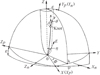 |
Fig. 1 Geometry of the precessing jet nozzle model adopted from Qian (2011). Three coordinate systems are used: (Xn, Yn, Zn), (X, Y, Z) and (Xp, Yp, Zp). The Yn axis is directed toward the observer and the Xn–Zn plane represents the sky plane. The (X, Y, Z) system is defined with respect to the (Xn,Yn,Zn) system and the precession axis (Z-axis) is defined by parameters (ϵ, ψ). The trajectory of a knot (superluminal component) is defined by parameters (A(Z), Φ) in the (X, Y, Z) system. θ denotes the angle between the knot’s velocity vector S and the direction toward the observer V; η is the initialhalf opening angle of the jet. (see text). |
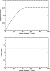 |
Fig. 2 Amplitude function A(Z) and precession phase Φ(Z) for describing the trajectory of knot C1. Its entire trajectory observed and kinematics can be well modeled in terms of the precessing nozzle model. |
2 Formalism of the model simulation (model fitting)
2.1 Geometry of the model
In order to perform the model simulation of the VLBI-kinematics of QSO 1302-102 in terms of a precessing nozzle model, we first give the description of the formalism of the model. Following Qian et al. (1991, 2009, 2014), we take the geometry of the model as shown in Fig. 1, in which three coordinate systems are used: (Xn, Yn, Zn), (X, Y, Z) and (Xp, Yp, Zp). The Yn -axis directs toward the observer and the (Xn, Zn) plane represents the sky plane: the Zn-axis is directed toward the north pole and the Xn axis is defined as the direction opposite to the direction of right ascension. The observed position angle of VLBI knots is measured in clockwise from the Zn-axis. The (X, Y, Z) system is used to define the trajectories of the components and defined with respect to the system (Xn, Yn, Zn) by parameters ϵ and ψ: ϵ denotes the angle between the Z-axis and Yn axis and ψ denotes the angle between the X-axis and Xn axis. The X-axis represents the intersection line of the (X, Y) plane and the (Xn, Zn) plane or directs toward the ascending node. The (Xp, Yp, Zp) system is introduced to make transformation between the (X, Y, Z) system and (Xn, Yn, Zn) system: the Xp axis coincides with the X-axis and Yp axis coincides with the Yn axis, and Zp axis is perpendicular to the (Xp, Yp)-plane. In the case of modeling the inner trajectories and kinematics of the superluminal components the Z-axis is regarded as the precession axis of the precessing nozzle model and the precession cone has a half opening angle of η. We assume that in the inner jet regions the superluminal knots move along individual collimated trajectories, which are defined by parameters (A(Z), Φ), as shown in Fig. 1. S denotes the direction of the speed vector and V denotes the direction toward the observer (parallel to the Yp -axis). θ denotes the viewing angle of the knot. We assume that in the inner jet regions each of the VLBI knots moves along a curved trajectory with a constant phase (Φ = constant), but for successive knots, the phase changes due to precession.
A curved trajectory is defined by parameters (A(Z), Φ), which describe the amplitude and the phase, respectively. Thus, a trajectory can be described in the (X, Y, Z) system as follows.

The projection of the trajectory on the sky plane is represented by

where ψ is the angle between the X(Xp)-axis and the Xn-axis,

We give the formulas for viewing angle θ, Doppler factor δ, apparent transverse velocity vapp, and elapsed time T after ejection as follows.
Viewing angle θ
![Mathematical equation: \begin{equation*} {\theta}=\arccos[\cos{{\mathrm{\Delta}}}(\cos{\epsilon}+ \sin{\epsilon}\tan{{{\mathrm{\Delta}}}_p})],\end{equation*}](/articles/aa/full_html/2018/07/aa32039-17/aa32039-17-eq4.png) (7)
(7)
where
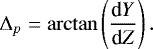
![Mathematical equation: \begin{equation*} {{\mathrm{\Delta}}}=\arctan\left[\left(\frac{\textrm{d}X}{\textrm{d}Z}\right)^2+ \left(\frac{\textrm{d}Y}{\textrm{d}Z}\right)^2\right]^{1/2}.\end{equation*}](/articles/aa/full_html/2018/07/aa32039-17/aa32039-17-eq5.png) (8)
(8)
Δ is the angle between the spatial velocity vector and the Z-axis and
 (9)
(9)
is the projection of Δ on the (Y, Z)-plane.
Apparent transverse velocity vapp and Doppler factor δ
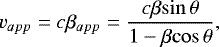 (10)
(10)
and
 (11)
(11)
where β = v∕c, v is the spatial velocity of the knot,  is the Lorentz factor.
Elapsed time T, at which the knot reaches the axial distance Z:
 (12)
(12)
and
![Mathematical equation: \begin{equation*} {{\mathrm{\Delta}}}_s=\arccos\left[\left(\frac{\textrm{d}X}{\textrm{d}Z}\right)^2+ \left(\frac{\textrm{d}Y}{\textrm{d}Z}\right)^2 +1\right]^{-1/2},\end{equation*}](/articles/aa/full_html/2018/07/aa32039-17/aa32039-17-eq11.png) (13)
(13)
z is the redshift of 1302-102 and Δs is the instantaneous angle between the velocity vector and the Z-axis. All coordinates and amplitude A(Z) are measured in units of mas. θ and v are instantaneous quantities atan elapsed time T.
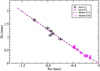 |
Fig. 3 KnotsC1 and C6 have almost equal position angles and move along very similar trajectories, but their observed ejection times are 1991.58 ± 0.28 and 2007.31 ± 0.30, differing by 15.73 yr. If this similarity of the position angles at the two ejection epoches is caused by the jet precession, then its is argued that 15.73/3 = 5.24 yr is the most appropriate precession period. The dotted and dashed lines denote the modeledtrajectories for knots C1 and C6, respectively (see text). |
2.2 Collimated trajectory and jet precession
In order to model fit the source kinematics, an appropriate formalism is needed to describe the motion of the superluminal components. We assumed that each of the VLBI components moves along a collimated trajectory with a constant precession phase (Φ = const.), but for successive knots, the phase changes due to precession. For this paper we chose the following form for describing the collimated trajectory of the knots.
The amplitude A(Z) of the collimated trajectory as a function of Z is taken as follows. When Z ≤ b,
 (14)
(14)
and when Z > b,
 (15)
(15)
Parameter b may be regarded as a “collimation parameter” to describe the form of jet collimation. The precession phase Φ is defined by the parameter ϕ for a specific trajectory as
 (16)
(16)
Φ0 is an arbitrary constant and ϕ is defined as the precession phase. Since dΦ∕dZ = 0, we have

And from Eqs. (8), (9), and (13) we have
![Mathematical equation: \begin{align}& {{\mathrm{\Delta}}}={\arctan\left(\frac{\textrm{d}A}{\textrm{d}Z}\right)},\\ & {{{\mathrm{\Delta}}}_p}={\arctan\left(\frac{\textrm{d}A}{\textrm{d}Z}\sin{{\mathrm{\Phi}}}\right)},\\ & {{{{\mathrm{\Delta}}}_s}}=\arccos\left(\left[1+ \left(\frac{\textrm{d}A}{\textrm{d}Z}\right)^2\right]^{-1/2}\right). \end{align}](/articles/aa/full_html/2018/07/aa32039-17/aa32039-17-eq16.png)
Substituting Δ, Δp and Δs into Equations (7), (10)–(12), we can calculate the viewing angle θ, apparent velocity βapp, Doppler factor δ and elapsed time T.
We have assumed a very simple pattern (shown in Fig. 2) of the common precessing trajectory for investigating the motion of the superluminal components, but it still closely represents the real jet structure configurations observed in radio galaxies and blazars. For example, the giant elliptic galaxy M87, having a powerful optical-radio jet and a supermassive black hole of ~ 6 × 10⁹ M⊙, is the best possible target for studying the initial jet formation and collimation process (Biretta et al. 2002). Nakamura & Asada (2013; also see Asada & Nakamura 2012 and Doeleman et al. 2012) found that the jet width can be well fitted by a parabola-like collimating profile in the core separation range from ~ 10 to ~ 105 Schwarschild radii and the jet has a single power-law structure starting from the vicinity of the supermassive black hole. They have also proposed a magnetohydrodynamic (MHD) nozzle model to interpret the property of the bulk jet acceleration, assuming that the MHD nozzle consists of a hollow parabolic tube (a simple and smooth structure without needing a complex configuration).
General relativistic MHD simulations (e.g., McKinney et al. 2012) reveal that magnetic field structures near the horizon of a rotating black hole closely correspond to a parabolic configuration which is consistent with the analytic results given by Beskin & Zheltoukhov (2013) for a field geometry: a radial field near the horizon and a vertical field far from the black hole. In these configurations, the distribution of the magnetic field and field angular velocity profile near the horizon can be described inmore details (Punsly 2001; McKinney et al. 2012; Beskin & Zheltoukhov 2013). In addition, Tateyama (2013) found that, in the prominent blazar OJ287, the superluminal components were ejected along a fork-like structure.
We have applied a similar approach to model fitting of the kinematics of the superluminal knots in blazars: 3C279 (Qian 2011, 2012), 3C454.3 (Qian et al. 2014) and B 1308+326 (Qian et al. 2017). In the following we investigate the kinematics of the superluminal knots in QSO 1302-102, assuming the simple pattern described above (Fig. 2) as the precessing common trajectory. In this paper we adopt the concordant cosmology model with ΩΛ = 0.73, Ωm = 0.27 and Hubble constant H0 = 71 km s−1 Mpc−1 (Hogg 1999; Pen 1999; Spergel et al. 2003). For QSO 1302-102, z = 0.278 (Marziani et al. 1996), its luminosity distance DL = 1.412 Gpc and angular diameter distance DA = 0.8645 Gpc. Angular scale of 1 mas = 4.19pc and proper motion of 1 mas yr−1 is equivalentto an apparent velocity of 17.46 c.
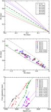 |
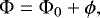
Fig. 4 Upper panel: modeled distribution of the trajectory of the precessing nozzle model for the inner jet regions. ϕ = 1.0, 2.0, 3.0, 4.0, 5.0, and 6.0 rad. The common trajectory rotates around the precession axis anticlockwise viewed along the axis. The precession axis is at position angle of 30.1°. Middle panel: distribution of the observed trajectories of knots C1–C6 in the plane of the sky. Bottom panel: model fitting of the core separations for knots C1–C6. The model fitting of their kinematics are shown individually in Figs. 5–10. |
3 Selection of model parameters
We simulate the kinematics of the superluminal components on parsec scales in 1302-102 during the period ~1990–2012 in terms of the precessing jet-nozzle model proposed by Qian et al. (1991, 2014). In order to investigate the jet position angle swing in 1302-102, the 15 GHz VLBI-data published in Kun et al. (2015) are used2. During the years ~1990–2012 six superluminal components were ejected (knots C1–C6).
The modeling approach and relevant formulae have been described in Sect. 2. The model-fitting approach is similar to those which have been applied previously to investigate the jet swings and kinematics for a few blazars: 3C345, 3C454.3, 3C279, NRAO 150 (Qian et al. 1991, 2014; Qian 2012, 2013, 2016), and B 1308+326 (Qian et al. 2017).
Jet swings (or wobblings) observed in blazars have been interpreted in terms of different mechanisms (e.g., Agudo 2009): (i) instabilities in accretion disk or jet for erratic jet swings; (ii) helical motion of superluminal components (shock-in-jet moving along a helical field); (iii) precession of the entire jet; and (iv) precession of jet nozzle. Usually, regular jet swings are explained in terms of precession mechanisms.
The precessing jet-nozzle model is different from the usual processing jet model. In the precessing jet model the whole jet precesses and all the superluminal knots ejected at different times move along the jet axis, forming an apparently helical jet pattern. However, in the precessing jet-nozzle model, the jet-nozzle precesses around a fixed precession axis (i.e., the symmetric axis of the jet-body) and the knots ejected from the nozzle at different times move along their own individual trajectories (plane or helical, Qian 2016) with different bulk Lorentz factors. The precession of the nozzle leads to the precession of the ejection direction of the knots or ejection position angle swing. The combination of a sequence of isolated knots ejected from this nozzle at different times would exhibit the structure of the entire jet and its structural evolution seen on VLBI-maps (e.g., Tateyama & Kingham 2004; Qian et al. 2009, 2014, 2017; Tateyama 2009; Qian 2012, 2013, 2016; Tateyama 2013; BQS17). The precessing nozzle model is usually applied to study the kinematics of inner-jet components and a precessing common trajectory is introduced for describing the inner trajectories of the superluminal components.
In orderto perform the model-fitting (or model simulation) of the kinematics of the superluminal components in terms of our precessing nozzle model, there are several model parameters should be set, including parameters (ϵ, ψ, A, b, Tp) for the overall model and parameters (t0, Γ, ϕ) for individual knots. Generally, we should choose different parameters for the inner-jet region and the outer jet region. In addition, these parameters can be divided into two sets as follows.
3.1 Geometric and kinematic parameters
For example, for investigating the kinematics of inner components, the Z-axis can be regarded as the precession axis and their trajectories follow a common trajectory shape. In this case the geometric and kinematic parameters include: (a) parameters ϵ and ψ defining the orientation of the precession axis (Z-axis) with respect to the observer system; (b) amplitude function A(Z) and collimation parameter b describing the shape of the precessing common trajectory with respect to the (X, Y, Z) system; (c) Lorentz factors (Γ) of the knots. Based on the observed kinematics of the knots, we are able to infer a preliminary set of parameters and through trial modelings to derive a final set of model parameters. For example, if the angle ϵ is given, then (i) the pattern of the common precessing trajectory (parameter A(Z) and b) can be roughly determined from the observed shapes of trajectories of the knots; (ii) the position angle of the precession axis can be estimated from the distribution of trajectories of the knots (taken as the axis of the symmetry of the distribution), and thus parameter ψ can be approximately estimated (see Figs. 3 and 4); (iii) the Lorentz factors (Γ) of the knots can be estimated from their observed apparent velocities. These parameters are not unique, mainly depending on the viewing angle of the precession axis (parameter ϵ), because viewing angle ϵ decides the projection effects and radial distance scales along the Z-axis. But they can be derived through trial model fittings of the kinematics of the knots using the formalism described in Sect. 2, which include the model-fittings of the trajectory Zn (Xn), core separation rn(t), coordinates Xn(t) and Zn (t) and apparent velocity vapp for each knot. When the value of parameter ϵ is given, a specific set of these parameters can finally derived. In this paper we have adopted ϵ = 1.5° which is similar to that (2.2° ± 0.5°) derived by Kun et al. (2015), based on the measurements of the brightness temperature of the VLBI-core.
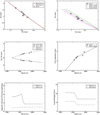 |
Fig. 5 Model fitting results of the kinematics for knot C1. It moves along the modeled precessing common trajectory during the whole observation period (core separation rn < 2 mas). In the upper right panel two additional modeled trajectories (green and magneta lines) calculated for the modeled ejection epoches t0 ± 0.5 yr (or ϕ ± 0.61 rad) are also shown, demonstrating that most of the observation data points are within the position angle range defined by the two additional modeled trajectories and the precession period is determined within an uncertainty of ~ ± 0.5 yr. |
3.2 Precession period Tp and related parameters
Generally, in the case for model fitting of the kinematics of superluminal components caused by jet precession, there are two methods to determine the precession period: (i) through trial model fittings of the kinematics of the superluminal components to select an appropriate period (e.g., Qian et al. 2017 for the quasar B 1308+326); (ii) by using the known periodicity found in optical bands (e.g.,Tateyama & Kingham 2004 for BLO OJ287). For the quasar PG 1302-102 there are some observational clues for helping select the precession period. For example, according to the observed distribution of trajectories of the superluminal knots C1–C6, the trajectories of knot C4 and knot C6 roughly form the edges of the jet cone (projected), having an aperture of ~ 11° (Table 2). Their ejection epochs are 2005.0 ± 0.2 and 2007.3 ± 0.3, respectively.The time difference of 2.3 yr implies that the precession period should be >4.6 yr, because the true precession cone should be larger than that formed by knots C4 and C6. Moreover, we found that knots C1 and C6 have similar (almost the same) ejection position angles and inner trajectories (Fig. 3). Their observed ejection epochs are 1991.58 ± 0.27 and 2007.31 ± 0.30, differing by 15.73 yr. Thus if the jet precession exists, then the possible period of precession which can be selected is one of the four values (one to fourth of 15.7 yr), that is, Tp = 15.7 yr, 15.7/2 = 7.85 yr, 15.7/3 = 5.23 yr, and15.7/4 = 3.93 yr, respectively. Obviously, the value 3.93 yr < 4.6 yr is not appropriate. The values of 15.7 and 7.85 yr (both much larger than 4.6 yr) imply that the jet cone is much larger than the observed one (formed by the trajectories of knot C4 and knot C6) and not valid either. Thus the value of 5.23 yr is the only one which can be selected as an appropriate precession period for the radio jet. Interestingly, this radio jet precession period, which is derived completely from radio observations, is almost exactly equal to the optical period found by Graham et al. (2015) in its optical light curve and explained by D’Orazio et al. (2015). This leads us to to think that there could be a relation between the radio jet swing and the optical variations. This becomes the main subject of this paper: through the model fitting of the source VLBI-kinematics to investigate the radio–optical relationship and the potential application of a supermassive black hole binary scenario.
Thus for the following model simulations we have selected the radio precession period to be 5.1583 yr (1884 days). This does not imply that the derivation of the radio jet precession period is dependent on the optical period. The radio jet precession period is purely determined from the VLBI observations, independent on the optical variability. This selection is just for convenience to discuss the radio-optical relationship caused by the jet precession of same period below.
We will show that the kinematics of all the six superluminal components can be consistently interpreted (or model–fitted) in terms of the precessing jet nozzle model proposed by Qian et al. (1991, 2009, 2014, 2017) with a precession period of 5.1583 ± 0.5 yr. Therefore the model fittings of the kinematics of all the six knots confirm the validity of the derived precession period.
We point out that the derivation of the geometric and kinematic parameters is not unique and depends on the choice of parameter ϵ which decides the projection effects and the source size scales. Different values chosen for ϵ lead to different sets of the geometric and kinematric parameters.
However, the precession period Tp and the ejection times t0 of the knots are strictly constrained by the observed ejection times (t0,obs) and the distribution of their position angles versus time (![Mathematical equation: $[PA(t)]_{obs}$](/articles/aa/full_html/2018/07/aa32039-17/aa32039-17-eq17.png) ). For the specified viewing angle ϵ = 1.5° adopted in this paper the parameters of the precessing nozzle model for the components moving in the inner jet regions are shown in Table 1 and all the parametrs are taken to be constants. For modeling the kinematics of the knots moving in the outer jet regions we have to introduce changes in parameter ψ, see below.
). For the specified viewing angle ϵ = 1.5° adopted in this paper the parameters of the precessing nozzle model for the components moving in the inner jet regions are shown in Table 1 and all the parametrs are taken to be constants. For modeling the kinematics of the knots moving in the outer jet regions we have to introduce changes in parameter ψ, see below.
The observed ejection times (t0,obs, Table 2) are obtained from VLBI measurements. For knots C1–C6, the differences between the modeled ejection times and the observed ones are +0.42 yr, +0.59 yr, − 0.46 yr, − 0.63 yr, − 0.42 yr, and +0.15 yr (see Table 2), respectively. These values are roughly within the error range (1 σ–2 σ) of the VLBI measurements, indicating that the modeled ejection times are acceptable. Similar analytical results can be seen from the model fitting of the jet swing for the radio galaxy 3C66B (Sudou et al. 2003).
When periodic position angle swings are investigated, there is always some problem about the discrepancy between themodeled ejection times and the observed ones. Which is physically more believable? In fact, the VLBI-measurements and the model fitting method are two different approaches for determining the ejection epoches. VLBI measurements are based on the linear regression method without consideration of the ingredients – for example, initial acceleration, trajectory curvature, opacity effects and insufficient data sampling within core separations less ~0.3–0.5 mas, while the precessing jet model fits concentrate on finding the precession period with consideration of these ingredients and fitting the source kinematics as well as possible. Usually, the observed and modeled ejection epoches differ by < ~ 0.5 yr. In some cases a difference of 1 yr or more is possible. For example, for one knot (knot-i) in QSO B1308+326, a discrepancy of ~1 yr between the modeled and observed ejection epoches was obtained (Qian et al. 2017). The flux variation of knot-i verified the modeled epoch, attributing the discrepancy to the initial acceleration and flux density evolution, confirming the applicability of the precessing nozzle model. Combining all the arguments given above, we come to the conclusion that the kinematics of the source 1302-102 can well be interpreted in terms of the precessing nozzle model with a precession period of ~ 5.16 ± 0.5 yr, very similar to the optical period claimed by Graham et al. (2015) in its optical light curve.
During the model fitting of the kinematics of the six knots we have thirty kinematic relations to be fitted (five relations for each knot). This is a procedure of fitting multiple kinematic relations with multiple parameters. Moreover, the observed ejection position angles (![Mathematical equation: $[{\rm{PA}}]_{obs}$](/articles/aa/full_html/2018/07/aa32039-17/aa32039-17-eq18.png) ) and ejection times (t0,obs) for the six knots are not sufficient to constitute a statistical sample, and standard statistical methods (e.g., Fourier transform and discrete autocorrelation) cannot be applied for an analysis of periodicity. Thus, the precession period can only be found through an analytical modeling of the kinematics of the knots (see Figs. 5–10 below). Therefore, the model fitting results obtained in this paper are tentative as one of the possible interpretations for the kinematics of the features in the jet of 1302-102. The model parameters we obtained are not unique, because they are derived for a specified viewing angle of the jet (ϵ = 1.5°), though the precessing period is strictly constrained by the change of the observed position angle of the knots with time, which is basically independent of the selection of the geometric and kinematic parameters.
) and ejection times (t0,obs) for the six knots are not sufficient to constitute a statistical sample, and standard statistical methods (e.g., Fourier transform and discrete autocorrelation) cannot be applied for an analysis of periodicity. Thus, the precession period can only be found through an analytical modeling of the kinematics of the knots (see Figs. 5–10 below). Therefore, the model fitting results obtained in this paper are tentative as one of the possible interpretations for the kinematics of the features in the jet of 1302-102. The model parameters we obtained are not unique, because they are derived for a specified viewing angle of the jet (ϵ = 1.5°), though the precessing period is strictly constrained by the change of the observed position angle of the knots with time, which is basically independent of the selection of the geometric and kinematic parameters.
The model parameters selected through the trial model fittings and the relevant modeled data are shown in Tables 1–2. The values measured for the parameters (position angle ![Mathematical equation: $[PA]_{obs}$](/articles/aa/full_html/2018/07/aa32039-17/aa32039-17-eq19.png) , ejection times
, ejection times  and apparent velocity βapp) are taken from the VLBI measurements by Kun et al. (2015).
In the fitting process, we set the following requirments to control the quality of the model fits: (i) the modeled ejection epochs of the knots are defined by the precession period as
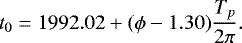 (22)
(22)
Here ϕ = 1.30 rad normalizes the ejection epochs to knot C1 (t0 = 1992.02); (ii) the trajectories, coordinates and core separations of the six knots are consistently fitted by visual inspection; (iii) the apparent velocities of the knots are well fitted; (iv) for the fits to the trajectories of the knots, most of the observational data points are within the position angle ranges defined by the two additional modeled trajectories calculated for epochs t0 +0.5 yr and t0 − 0.5 yr, indicating the precession period being determined within an uncertainty of ~ ± 0.5 yr (see the magneta and green lines in the upper/left plots of Figs. 5–10). This condition may be regarded as our main criteria to judge the correctness of the precession period derived.
The modeled and observed ejection times are given Table 2. In the upper panels of Fig. 4 are shown the distributions of the modeled and observed trajectories, respectively. The model fitting of the core separations versus time for knots C1−C6 is shown in the lower panel of Fig. 4.
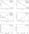 |
Fig. 6 Model fitting results of the kinematics for knot C2. Within core separation rn < 1.47 mas, ψ = constant = − 2.097 and knot C2 moves along the modeled precessing common trajectory. In the upper left panel the dashed red line (modeling the entire trajectory) and the solid black line (modeling the inner trajectory) coincide within core separation rn < 1.47 mas, showing a small curvature in its outer trajectory. In the upper right panel two additional modeled trajectories calculated for t0 ± 0.5 yr (or ϕ ± 0.61 rad) are added todemonstrate that most of the observation data points are within the position angle range defined by the two additional modeled trajectories (green and magneta lines) and the precession period is determined within an uncertainty of ~ ± 0.5 yr. |
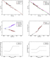 |
Fig. 7 Results of the model fitting of the kinematics for knot C3. Within core separation rn < 1.19 mas its inner trajectory follows the precessing common trajectory. In the upper left panel the red dashed line (modeling the entire trajectory) and the solid black line (modeling the inner trajectory) coincide within core separation rn < 1.19 mas, showing the curvature in its outer trajectory. In the upper right panel two additional modeled trajectories (green and magneta lines) for ejection epoches t0 ± 0.5 yr (or ϕ ± 0.61 rad) are also added, demonstrating that most of the observation data points are within the position angle range defined by the two additional modeled trajectories and the precession period is determined within an uncertainty of ~ ± 0.5 yr. |
Parameters selected for the precessing nozzle model for modeling the inner trajectories and kinematics.
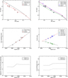 |
Fig. 8 Modeling results of the kinematics for knot C4. It moves along a curved trajectory with small oscillations. Its inner trajectory and kinematics can be well fitted by the precessing nozzle model within core separation rn < 0.58 mas. In the upper left panel the solid black line (modeling the inner trajectory) and the dashed red line (modeling the entire trajectory) coincide within core separation of 0.58 mas, showing the curvatures in its outer trajectory. In the upper right panel two additional modeled trajectories are shown for ejection epochs t0 ± 0.5 yr, demonstrating that most of the observation data points are within the position angle range defined by the two trajectories (green and magneta lines) and the precession period is determined within an uncertainty of ~ ± 0.5 yr. |
Precessing nozzle model parameters for the inner trajectories and kinematics.
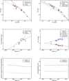 |
Fig. 9 Modeling results of the kinematics for knot C5. It moves along a curved trajectory and the data points from Lister et al. (2009 for knot C6, designated as LC6 here) are added to check its initial trajectory pattern. In the upper left panel the dashed red line (modeling the entire trajectory) and the solid black line (modeling the inner trajectory) coincide within core separation rn < 1.04 mas, evidently showing the transition from the precession common trajectory to the curved trajectory in the outer jet region. In the upper right panel two additional modeled trajectories calculated for ejection epoches t0 ± 0.5 yr (or ϕ ± 0.61 rad), demonstrating that most of the observation data points are within the position angle range defined by the two additional modeled trajectories (green and magneta lines) and the precession period is determined within an uncertainty of ~ ± 0.5 yr. |
4 Model fitting results for individual knots
The fitting results are shown in Figs. 5–10 for the jet components, individually. It can be seen that the kinematics of all the six superluminal features are well fitted by the precessing nozzle model with the assumed set of model parameters discussed in Sect. 3. For each knot, three modeled trajectories are given, which are obtained for the ejection time t0 and two additional epoch times of t0 ± 0.5 yr, corresponding to the precession phase ϕ and ϕ ± 0.61 rad, respectively.The aim is for demonstrating that most of the observational data points are within the position angle ranges defined by the two additional modeled trajectories (magneta and green lines). Thus, we provide some evidence for the radio precession period being determined within an uncertainty of ~ ± 0.5 yr.
In the following we will model the observed kinematics of the superluminal knots individually. We find that the inner trajectories of the knots can be consistently fitted in terms of the precessing nozzle model. That is, their inner trajectories can be modeled by the precession of a common trajectory: their shape and motion has a common axis (i.e., the precession axis defined by the parameters ϵ = 1.5° and ψ = − 2.097 rad = − 120.16°, see Table 1). However, their outer trajectories are found to be deviated from the precessing common trajectory, that is, trajectory curvatures in the outer jet regions need to be taken into account. In these outer regions the motion of the knots will not have a common axis and shape for their outer trajectories. In order to consider the model fits of the outer trajectories we need to choose the model-fitting parameters for the knots individually. Generally, changes in parameters ϵ, ψ, A(Z) or ϕ are all possible, and could be introduced to model their outer trajectories (Qian et al. 2017)3. For simplicity, in this paper we introduce variations in parameter ψ in the outer jet regions to model their outer trajectories, that is, the outer trajectory curvatures of the knots can be described by using values of ψ different from the common value (− 2.097 rad) for their inner trajectories. In this case there are no common precession axis and common precessing trajectory existing for the description of the individual knot motion. In the case of ϵ = constant (see Fig. 1) the changes in ψ represent rotations of their outer trajectories about the viewing axis (Yn -axis) in the observer system. This implies that our model fitting of the source kinematics includes two parts: the precessing nozzle model reproduces the inner trajectories of the knots and their outer trajectories are model fitted by introducing additional trajectory curvatures. There is a transition of the trajectory-pattern of the knots from the precessing common trajectory in the inner-jet regions to the individual trajectory patterns in the outer-jet regions.
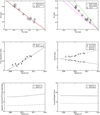 |
Fig. 10 Model fitting results for knot C6. Knot C6 moves along the precessing common trajectory during the whole observation period. In the upper left panel the solid black line (modeling the inner trajectory) and the dashed red line (modeling the entire trajectory) coincide. In the upper right panel three modeled trajectoryies are shown for t0 (black dashed line) and t0 ± 0.5 yr (or ϕ ± 0.61 rad; green and magneta lines), demonstrating that most of the observation data points are within the position angle range defined by the two additional modeled trajectories and the precession period is determined within an uncertainty of ~ ± 0.5 yr. |
4.1 Model fitting for knot C1
The modeling results for the kinematics of knot C1 are shown in Fig. 5: trajectory Zn (Xn), coordinates Xn(t) and Zn(t), core separation rn(t), the modeledapparent velocity and viewing angle, and the modeled Lorentz/Doppler factor. Its modeled ejection epoch t0 = 1992.02 and the cooresponding precession phase ϕ = 1.30 rad.
In the inner jet region with core separation rn < 2 mas (or Z < 82 mas) the trajectory and kinematics of knot C1 can be well fitted by the precessing nozzle model during the whole observation period and apparently has a rectilinear motion. Thus in the upper left panel of Fig. 5 the solid black line (modeling the inner trajectory) and the dashed red line (modeling the entire trajectory) coincide.
In the upper right panel two additional model trajectories (green and magneta lines) calculated for ejection times t0 ±0.5 yr (or ϕ ± 0.61 rad) are also shown, demonstrating that most of its observational data points are within the position angle range defined by the two additional model trajetories and the precession period is determined within an uncertainty of ~ ±0.5 yr.
In order to explain its core separation versus time deceleration of its motion after 1995 is required: For Z < 50 mas (or core separation rn < 1.16 mas) Γ = 11.2; For Z = 50–60 mas Γ = 11.2–4(Z − 50)∕(60–50); For Z > 60 mas Γ = 7.2. Thus the modeled apparent velocity changes from ~5.1 c to ~2.6 c, showing its apparent deceleration after 1995.
4.2 Model fitting for knot C2
The fitting results for the kinematics of knot C2 are shown in Fig. 6: trajectory Zn (Xn), coordinates Xn(t) and Zn(t), core separation rn(t), the modeled apparent velocity and viewing angle, and the modeled Lorentz/Doppler factor. Its modeled ejection epoch t0 = 1994.79 and the corresponding precession phase ϕ = 4.67 rad.
Knot C2 was observed within a core separation of ~3.9 mas and has a slighly curved trajectory in the outer region. In the inner jet region with core separation rn < 1.47 mas (Z < 50 mas) the (inner) trajectory of knot C2 can be well fitted by the precessing nozzle model with ψ = − 2.097 rad. In the upper left panel of Fig. 5 the dashed red line (modeling the entire trajectory) and the solid black line (modeling the inner trajectory) have only a small difference on the outer separations.
Its outer trajectory and kinematics can be modeled by introducing slight changes in parameter ψ: For Z = 50–160 mas ψ(rad) = − 2.097–0.01(Z–50)/(160–50); For Z > 160 mas ψ(rad) = − 2.1074. In the upper left panel of Fig. 6 the model fit with considering the outer trajectory curvatures coincides with the precessing model line in the inner region (rn < 1.47 mas or Z < 50 mas) and a slight deviation from the precessing model line beyond this separation.
In the Fig. 6 the data points from Lister et al. (2009 for knot C4, designed as LC4 here) are added to check its inner trajectory pattern. In the upper/right panel two additional model trajectories for ejection epochs t0 ±0.5 yr (or ϕ ± 0.61 rad) demonstrate that most of the observation data points are within the position angle range defined by the two additional model trajectories and the precession period is determined within an uncertainty of ~ ±0.5 yr.
In orderto explain its core separation versus time deceleration of its motion after 1996 is taken into account: For Z ≤ 20 mas, Γ = 10.6; For Z = 20–50 mas Γ = 10.6–1.3(Z − 20)/(50–20); For Z > 50 mas, Γ = 9.3 5. The modeled apparent velocity changes from ~6.3 c to ~4.3 c, showing its apparent deceleration after 1996.
4.3 Model fitting for knot C3
The model fitting results of the kinematics for knot C3 are shown in Fig. 7, including trajectory Zn (Xn), coordinates Zn(t) and Xn(t), core separation rn(t), the modeled apparent velocity and viewing angle, and the modeled Lorentz/Doppler factor. Its modeled ejection epoch t0 = 2000.04 and the corresponding precession phase ϕ = 4.78 + 2π. The data-points from Lister et al. (2009 for knot C4, designated as LC4) are also added to check the curvature of its trajectory in the outer jet region.
Knot C3 was observed along a curved trajectory with small-amplitude oscillations. In the inner-jet region with core separation rn < 1.19 mas (or Z < 40 mas) it moves along the modeled precessing common trajectory and its inner trajectory and kinematics can be well fitted by the precessing nozzle modelcan be well fitted by the precessing nozzle model (ψ = constant = − 2.097 radians). Beyond this separation or in the outer jet region its trajectory deviates from the common trajectory predicted by the precessing model and its outer trajectory can be fitted by introducing the changes in parameter ψ: For Z = 40–80 mas ψ(rad) = − 2.0970.05(Z − 40)/(80–40); For Z = 80–150 mas ψ(rad) = − 2.147 + 0.03(Z − 80)/(150–80); For Z > 150 mas ψ(rad) = − 2.117.
In the upper left panel of Fig. 7 we plot the model-fit of the inner trajectory and that of the entire trajectory. In the upper right panel of Fig. 7 two additional modeled trajectories (green and magneta lines) are shown for ejection epoches t0 ± 0.5 yr (or ϕ ± 0.61 rad), demonstrating that most of the observation data points are within the position angle range defined by the two additional modeled trajectories and the precession period being determined within an uncertainty of ~ ±0.5 yr.
In order to explain the variation of its core separation with time the motion of knot C3 has to be modeled as accelerated with the Lorentz factor changing from 9 to 14: for Z < 40 mas Γ = 9.0; For Z = 40–80 mas Γ = 9.0 + 5(Z− 40)/(80–40); For Z > 80 mas Γ = 14.0. The modeled apparent velocity varies in the range from ~4.5 c to ~9.0 c.
4.4 Model-fitting for knot C4
The model fitting results of the kinematics for knot C4 are shown in Fig. 8, including trajectory Zn (Xn), coordinates Zn (t) and Xn (t), core separation rn (t), the modeled apparent velocity and viewing angle, and the modeled Lorentz/Doppler factor. Its modeled ejection epoch is 2004.37 and the corresponding precession phase ϕ = 3.78 + 4π. The data-points from Lister et al. (2009 for knot-C5, designed as LC5 here) are added to check the curvature of its trajectory.
Knot C4 was observed to move along a curved trajectory with small-amplitude oscillations. In the inner-jet region with core separation rn < 0.58 mas (or Z < 20 mas) its (inner) trajectory and kinematics can be well fitted by the precessing nozzle model (ψ = constant = − 2.097 radians). Beyond this separation its outer trajectory deviates from the trajectory predicted by the precessing nozzle model and its trajectory and kinematics are fitted by introducing the changes in ψ: For Z = 20–35 mas ψ(rad) = − 2.097–0.08(Z − 20)/(35–20); For Z = 35–100 ψ(rad) = − 2.177 + 0.06(Z − 35)/(100–35); For Z > 100 mas ψ(rad) = − 2.117.
In the upper left panel of Fig. 8 we plot the model fit of the inner trajectory and that of the entire trajectory with introduction of changes in ψ in the outer jet region. In the upper right of Fig. 8 two additional model trajectories (green and magneta lines) are shown for ejection times t0 ± 0.5 yr (or ϕ ± 0.61 rad), demonstrating that most of the observation points are within the position angle range defined by the two additional model trajectories and the precession period being determined within an uncertainty of ~ ±0.5 yr.
To explain the variation of the core separation with time Its motion has to be modeled as accelerated: For Z < 20 mas Γ = 10; For Z = 20–35 mas Γ = 10 + 2(Z − 20)/(35–20); For Z > 35 mas Γ = 12. Its modeled apparent velocity changes from ~5 c to ~7 c which is comparable to 7.2 ± 0.7 c given by Kun et al. (2015).
4.5 Model fitting for knot C5
The model fitting results of the kinematics for knot C5 are shown in Fig. 9, including trajectory Zn (Xn), coordinates Zn(t) and Xn(t), core separation rn(t), the modeledapparent velocity and viewing angle, and the modeled Lorentz/Doppler factor. Its modeled ejection epoch t0 = 2004.69 and the corresponding precession phase ϕ = 4.17 + 4π. The data-points from Lister et al. (2009 for knot C6, designed as LC6 here) are added to check the curvature of its trajectory.
Knot C5 was observed to move along a curved trajectory which is the most evident one among the six knots. In the inner-jet region of core separation rn < 1.04 mas (or Z < 35.1 mas) its (inner) trajectory can be well fitted by the precessing nozzle model (ψ = constant = − 2.097). Beyond thisseparation its (outer) trajectory deviates from the trajectory predicted by the precessing model and its outer kinematics can be explained by introducing the changes in ψ: For Z = 35–100 mas ψ(rad) = − 2.097–0.25(Z − 35)∕(100 −−35); For Z > 100 mas ψ(rad) = − 2.347.
In the upper left panel of Fig. 9 we plot the model fit of the inner trajectory and that of the entire trajectory, considering the changes in ψ in the outer jet region. In the upper right panel of Fig. 9 two additional modeled trajectories (green and magenta) are shown for ejection epochs t0 ± 0.5 yr (or ϕ < 0.61 rad), demonstrating that most of the observation data-points are within the position angle range defined by the two additional model trajectories and the precession period being determined within an uncertainty of ~ ±0.5 yr.
Its variation of core separation with time can be roughly explained if its motion is assumed to be uniform: Γ = const. = 8.4. Its modeled apparent velocity changes in the range 3.5–4.0 c, which is consistent with the value (4.2 ± 0.9 c) given by Kun et al. (2015).
4.6 Model fitting for knot C6
The fitting results for knot C6 are shown in Fig. 10, including trajectory Zn (Xn), coordinates Zn(t) and Xn(t), core separation rn(t), the modeled apparent velocity and viewing angle, and the modeled Lorentz/Doppler factor. Its modeled ejection epoch t0 = 2007.45 and the corresponding precession phase ϕ = 1.24 + 6π. The trajectory and kinematics of knot C6 can be well fitted by the precessing nozzle model (ψ(rad) = − 2.097) for the whole observation time period (core separation rn < 0.75 mas or Z < 33.3 mas). Thus in the upper left panel of Fig. 9 the solid black line (modeling the inner trajectory) and the dashed red line (modeling the entire trajectory) coincide.
In the upper right panel of Fig. 9 two additional modeled trajectories (green and magneta lines) are shown for ejection epoches t0 ± 0.5 yr (or ϕ ± 0.61 rad), demonstrating that most of the observation data-points are within the position angle range defined by the two additional modeled trajectories and the precession period being determined within an uncerainty of ~ ±0.5 yr.
The variation of its core separation with time can be fitted if its motion is modeled as uniform with Γ = const. = 8.6. Its modeled apparent velocity changes from ~3.0 c to ~3.6 c, which is comparable to that (3.0 ± 0.4 c) derived by Kun et al. (2015).
4.7 A brief summary
Based on the model fitting results shown in Figs. 5–10, we have shown that (i) the position angle swing of the radio jet in PG 1302-102 is periodic with a precession period of 5.1583 ± 0.5 yr; (ii) the kinematics of all the six superluminal components can be consistently interpreted in terms of the precessing jet nozzle model proposed by Qian et al. (1991, 2009, 2014); (iii) their inner trajectories follow the modeled precessing common trajectory. The outer trajectories of knots C2, C3, C4, and C5 are curved with slight oscillations and changes of the parameter ψ are introduced for explaining this behavior; (iv) the variations in ψ in the outerregions imply that the trajectories of the knots rotate about the viewing axis (Yn -axis) in the observerframe and they have undergone a transition from the precessing common trajectory pattern to their individual trajectory patterns; (v) in order to demonstrate the validity of the precessing nozzle model for the inner trajectories of the knots in Table 3 we list the core separations within which their inner jet kinematics can well be fitted in terms of theprecessing nozzle model. It can be seen that for different knots this core separation is different: from ~0.75 mas (knot C6) to ~2 mas (knot C1), corresponding to axial distances along the precession axis from ~33.3 mas (140 pc) to ~82 mas (340 pc). Thus we find that in a distance range of 100–300 pc PG 1032-302 may have a very regular kinematic behavior which can well described by our precessing nozzle model with a precession period of ~5.16 yr. Obviously, this may imply a long-scale collimation and acceleration zone in this blazar, as suggested for 3C345 (Vlahakis & Königl 2004); (vi) for knots C1–C4 deceleration or acceleration of their motion are required for fitting their core separation versus time. These kinematic features of the knots observed in PG 1302-102 are generally consistent with those observed in generic blazars as discussed by Homan et al. (2015); (vii) the modeled Lorentz factors derived in this work are in the range Γ ~ 8–11.
The top panel of Fig. 11 shows the relation between the modeled ejection position angle and the modeled viewing angle for the six knots. It can be seen that the modeled viewing angle changes in a range of 0.54° (from 1.23° to 1.77°) and the modeled position angle in a range of 20° (from 20° to 40°). The modeled ejection position angles of the knots are shown in the middle panel of Fig. 11. As shown in Table 2, the differences between the modeled and observed ejection position angles of the knots ![Mathematical equation: $\mid[\textrm{PA}]_{obs}$](/articles/aa/full_html/2018/07/aa32039-17/aa32039-17-eq22.png) –PA∣ are in the range of 0.1°–1.8°, indicating that the observed ejection position angles are well fitted. The observed ejection times (tobs) of the knots are reasonably well fitted by the modeled ejection times (t0) within the range of the measurement errors of ~0.1−0.7 yr. Moreover, Figs. 5–10 reveal that the inner trajectories and kinematics of all the six components are well fitted by the precessing model and most of their observational data points are within the position angle ranges defined by the two additional modeled trajectories (green and magenta lines) calculated for ejection epochs t0 + 0.5 yr and t0 − 0.5 yr, indicating that the precessing period is determined within an uncertainty of ~ ± 0.5 yr. In the bottom panel of Fig. 11 the 15 GHz light curves of the source and the core, and the Doppler beaming ratio
–PA∣ are in the range of 0.1°–1.8°, indicating that the observed ejection position angles are well fitted. The observed ejection times (tobs) of the knots are reasonably well fitted by the modeled ejection times (t0) within the range of the measurement errors of ~0.1−0.7 yr. Moreover, Figs. 5–10 reveal that the inner trajectories and kinematics of all the six components are well fitted by the precessing model and most of their observational data points are within the position angle ranges defined by the two additional modeled trajectories (green and magenta lines) calculated for ejection epochs t0 + 0.5 yr and t0 − 0.5 yr, indicating that the precessing period is determined within an uncertainty of ~ ± 0.5 yr. In the bottom panel of Fig. 11 the 15 GHz light curves of the source and the core, and the Doppler beaming ratio ![Mathematical equation: $[{{\delta}_{max}}/{{\delta}_{min}}]^3$](/articles/aa/full_html/2018/07/aa32039-17/aa32039-17-eq23.png) are shown (for an assumed radio spectral index αr = 0 and Lorentz factor Γ = 10), indicating that the radio flux variability is not correlated with the Doppler beaming and can not be explained by using the jet precession. We also indicate the ejection epoches of the knots.
are shown (for an assumed radio spectral index αr = 0 and Lorentz factor Γ = 10), indicating that the radio flux variability is not correlated with the Doppler beaming and can not be explained by using the jet precession. We also indicate the ejection epoches of the knots.
Core separations rn (mas) and thecorresponding distance Z (mas and pc) along the precession axis within which the inner trajectories of the knots are well fitted in terms of the precessing nozzle model with a precession period of ~5.16 yr.
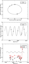 |
Fig. 11 Some relations for the inner precessing nozzle model. Top panel: modeled relation between the ejection position angle and the initial viewing angle, denoting the PA range of ~ 20° (from 20° to 40°) and the viewing angle range of ~ 0.54° (from 1.23° to 1.77°). The precession axis is at (30.14°, 1.50°). Middle panel: Modeled PA(t) and the modeled position angles of knots C1–C6. Lower panel: flux density variations of the VLBI-core and the total source at 15 GHz and the Doppler beaming ratio
|
![Mathematical equation: $[{{\delta}}/{{\delta}_{min}}]^3$](/articles/aa/full_html/2018/07/aa32039-17/aa32039-17-eq52.png)
5 Relationship between radio jet swing and optical variability
5.1 Introduction
In the above, we have shown that the radio inner jet of PG 1302-102 is precessing with a period of 5.1583 ± 0.5 yr. This period is derived completely from the radio (VLBI) observations during the monitoring period 1995–2012. Our analyses and model fittings indicate that the kinematics of all the six superluminal components on pc-scales can be consistently and well fitted (simulated) in the terms of the precessing nozzle and common trajectory model (Qian et al. 1991, 2009, 2014, 2017; Qian 2011, 2012, 2013, 2016). However, the precessing jet nozzle model proposed for interpreting the radio jet position angle swing cannot explain the optical variability in PG 1302-102 with the observed amplitude of Fopt,max∕Fopt,min ≃ 1.3 (Graham et al. 2015): Since the observed optical spectral index αopt is +1.1 (F0 ∝  in the rest frame), the optical variability amplitude due to the Doppler boost caused by the jet precession will be Fopt,max∕Fopt,min =
  . The variability amplitude derived from the precessing jet model is <1.2 (for Γ = 8–11), which is less than the observedamplitude ~1.3. We also notice that the precessing jet model suggested by Graham et al. (2015) for a viewing angle of 5° cannot explain the observed optical variability either if adopting the observed optical spectral index αopt = +1.1 instead of −1.66 which they used.
Therefore, the most plausible mechanism may involve a binary system of two supermassive black holes, as suggested by D’Orazio et al. (2015). They have proposed a specific binary black hole model to explain the periodic optical variability. Since the observed optical/UV spectral distribution has a UV-bump like pattern, they assume that its optical/UV emission is dominated by the emission from the accretion disk of the secondary hole and the periodic variability is due to the Doppler boosting caused by its orbital motion. They also provide some observational evidence for correlated variations in near-UV (NUV) and far-UV (FUV) bands. We note that according to D’Orazio et al. (2015) the spectral indices in the NUV and FUV bands are − 1.05 and − 2.0 the amplitudes of variability in NUV and FUV bands are ~30% and ~37%, higher than in the optical band (~14%) by a factor 2–2.5. This possible correlated variation in optical, NUV and FUV bands seems very important for the binary hole model, but it needs to be tested by future high-quality monitoring observations. In order to understand why the radio jet precession and the optical variability observed in PG 1302-102 have the same period of 5.2 yr the most appropriate and plausible way may be to investigate how the radio jet precession can be explained in terms of a binary black hole scenario.
5.2 Mechanisms for jet precession
In order to study the relationship between the radio jet precession and the periodic optical variability observed in PG 1302-102 we have to investigate the interpretation of the radio jet precession. Several mechanisms (e.g., Begelman et al. 1980a; Roos et al. 1993; Scheuer & Feiler 1996; Britzen et al. 2001; Tateyama & Kingham 2004; Caproni et al. 2006; Qian et al. 2014) have been proposed to interprete the precession of jets on parsec-scales in blazars. These may be divided into two categories: single black hole scenario and binary black hole scenario.
5.2.1 Single black hole scenario
Two mechanisms have been proposed: (a) Spin-induced precession (Lense-Thirring precession): due to the inertial frame-dragging effect of the central rotating (Kerr) black hole the jet associated with an inclined (or disaligned) disk will precess around the spin axis of the hole (e.g., Lense & Thirring 1918; Bardeen & Petterson 1975; Scheuer 1992; Scheuer & Feiler 1996; Nelson & Papaloizou 2000; Liu & Melia 2002; Caproni et al. 2004b; Qian et al. 2014, 2017); (b) Disk-driven precession: The jet aligned with a black hole and its innermost disk could precess due to the inertial dragging effect (Lense- Thirring effect) from its sufficiently massive outer disk (e.g., Sarazin et al. 1980; Lu 1990).
5.2.2 binary black hole scenario
This scenario have three distinct mechanisms: (a) Geodetic precession: the spin axis and the aligned jet of a Kerr black hole moving in a circular orbit will be precessed by the spin-orbit coupling and space curvature from the companion (Begelman et al. 1980a, 1980b; Thorne & Blandford 1982; Caproni et al. 2004a); (b) Newtonian-driven precession: the accretion disk and its aligned jet of a black hole inclined to the orbital plane will be precessed by the orbital motion of the companion via its gravitational torque on the disk (e.g., Katz 1997; Britzen et al. 2001; Tateyama & Kingham 2004; Lobanov & Roland 2005; Valtonen & Wiik 2012; Roland et al. 2013, 2015; Valtonen& Pihajoki 2013); (c) orbital motion of a binary: The periodically changing orbital velocity direction of a jet-launching black hole will cause the precession of the jet as seen by a distant observer due to the composition of the jet-launching velocity and the orbital velocity (Roos et al. 1993; Kun et al. 2015; Britzen et al. 2017, Qian et al. 2017).
While the single black hole scenario can be applicable to explain the radio jet swing in PG 1302-102, the optical periodicity can only be explained in terms of the binary black hole scenario. So we restrain our discussion on the binary black hole mechanisms. However, among the mechanisms suggested for jet precession, some mechanisms, for example, geodetic precession in a binary system, give precession periods of ~ 104 years, which are too long to be applicable to explain the precession period (~4.0 yr, in the source frame) found in 1302-102. The Newtonian driven precession mechanism may encounter the problem of unstable disk of the primary hole (e.g., Qian et al. 2017).
Therefore, in the following we will concentrate on the investigation of the possibility of interpreting the radio jet swing and the position angle distribution of the superluminal componentsin in terms of the orbital motion of a black hole binary. We assume that QSO 1302-102 harbors a supermasssive black hole binary and the primary hole is the jet emitter and the radio jet swing is originated from the orbital motion of the primary hole.
5.3 Orbital motion of the primary hole
In a binary black hole system the jet-producing black hole (designated as the primary black hole with mass M) moves around the mass-center of the system and the orientation of the jet will be modulated by its orbital motion due to the composition of the jet-launching velocity and the orbital velocity (e.g., Roos et al. 1993; Kun et al. 2015; BQS17).
The orbital period Torb of a binary is given as below: (e.g., Begelman et al. 1980a; Shapiro & Teukolsky 1983; Lang 2002)
![Mathematical equation: \begin{equation*} {T_{orb}}={\biggl[\frac{4{\pi}^2{r^3}}{G(M+m)}\biggr]}^{\frac{1}{2}}, \end{equation*}](/articles/aa/full_html/2018/07/aa32039-17/aa32039-17-eq26.png) (23)
(23)
or
 (24)
(24)
Here, M8 and m8 are the masses of the primary and secondary holes in units of 108 M⊙, rpc is the separation of the binary in units of pc, G is the Newtonian gravitational constant. The binary separation can be written as
![Mathematical equation: \begin{equation*} {r_{pc}}\,{\simeq}\,2.4\times10^{-3}{\biggl[\frac{T_{orb}}\textrm{yr}\biggr]}^{2/3} {({M_8+m_8})^{1/3}}. \end{equation*}](/articles/aa/full_html/2018/07/aa32039-17/aa32039-17-eq28.png) (25)
(25)
Correspondingly, the post-Newtonian parameter ϵ1 is
 (26)
(26)
We assume that the primary hole is the jet-emitter and its orbital velocity vorb,M around the center of mass is expressed as
 (27)
(27)
or
![Mathematical equation: \begin{equation*} {v_{orb,M}}={\frac{q}{1+q}}\biggl[2{\pi}{G(M+m)}/{T_{orb}}\biggr]^ {\frac{1}{3}}. \end{equation*}](/articles/aa/full_html/2018/07/aa32039-17/aa32039-17-eq31.png) (28)
(28)
Here q = m∕M is the mass ratio of the binary and thus
 (29)
(29)
Here, βorb,M = vorb,M/c and the orbital velocity of the secondary hole is vorb,m = vorb,M/q.
In order to produce the jet precession due to the orbital motion of the primary hole, its orbital velocity βorb,M should satisfy the following condition:
 (30)
(30)
Here, the orbital velocity component perpendicular to the jet axis (or the the axis of the primary disk) is  =
=  . βj = vj /c, vj is the jet launching velocity, c is the speed of light, η is the half opening angle of the jet precession cone, i is the inclination of the primary disk to the orbital plane (or the angle between the orbital angular momentum and the axis of the primary disk –or jet–)6. ω is the orbital phase. In order to specifically investigate the jet precession due to the orbital motion of the primary hole, different inclinations of the orbital plane with respect to the primary disk need to be considered.
5.4 Derivation of parameters for different inclinations
D’Orazio et al. (2015) has proposed a binary hole model to explain the periodicity of the optical variability in 1302-102. Based on hydrodynamic and magnetohydrodynamic simulations (e.g., Farris et al. 2014; Shi & Krolik 2015; Shi et al. 2012; D’Orazio et al. 2013), they proposed that PG 1302-102 harbors a supermassive black hole binary, containing three distinct optical emission components: a circumbinary disk, an accreting circumprimary disk and an accreting circumsecondary disk7. They also assumed that the optical emission is dominated by the emission from the accretion disk of the secondary black hole, the accretion rate of which is much larger than that of the primary hole (ṁ ∕Ṁ ≃ 20). The periodic optical variability with a period of ~5.2 yr is caused by the orbital motion of the secondary hole and the variability amplitude of ~13.5% is originated from the Doppler boost due to the motion of the secondary hole. In this case the observed optical variability amplitude is determined by the maximum radial velocity of the secondary hole, that is,
 (31)
(31)
Here, βorb,m is the orbital velocity of the secondary hole. In order to explain the observed optical variability amplitude 13.5% (for optical index αopt = +1.1), the required βorb,m should be:
 (32)
(32)
D’Orazio et al. (2015) analyzed the relation between the angle i and the parameters q and M + m, presenting the results in their Fig. 1 for the total mass range from 109.0 M⊙ to 109.4 M⊙, which was derived by Graham et al. (2015) from the measurements of broad emission lines.
In order to explain the radio jet precession the motion of the primary hole should also satisfy some conditions. In this case the jet precession is determined by the perpendicular component of its orbital velocity
 (33)
(33)
Its maximum value is equal to βobs,M (ω = 90°) and the minimum value is βobs,M cosi (ω = 0°). They will decide the scale of the elliptic precession cone with the axial ratio (minor-axis/major-axis equal to cos i). Assuming that the half opening angle of the precession cone (η = 0.275°) derived from the model fitting of the source kinematics is related to the maximum perpendicular velocity component of the primary hole, we then obtain
 (34)
(34)
As both the velocities of the primary and secondary holes are derived, parameters M, m and q of the binary can be estimated from the following equations.
 (35)
(35)
and
![Mathematical equation: \begin{equation*} {M_8+m_8}=4.12 \times 10^4 {[{{\beta}_{obs,m}}(1+q)]^3} .\end{equation*}](/articles/aa/full_html/2018/07/aa32039-17/aa32039-17-eq41.png) (36)
(36)
In Table 3 the relevant parameters (m, M, q, r, and ϵ1) are listed for inclinations i = 40°, 50°, 60° and 70°. It can be seen from Table 4 that the total mass of the binary is in the range of [6.3, 2.1] × 109 M⊙ with q in the range [0.04, 0.06], depending on the orbital inclination: the total mass of the binary increases with the decrease of the inclination angle.
As well known orbital motion may provide the best way to measure the parameters of a binary system (e.g., the black hole mass of the Galaxy center, Gebhardt et al. 2011). In the case of PG 1302-102 the combination of the jet precession and the periodic optical variability caused by the motion of a black hole binary might have provided a new approach to measure the parameters of the binary through its orbital motion. Therefore the investigation of the possible correlation between the periodic optical variability and the radio jet precession may be meaningful for understanding the physical processes in blazars.
For PG 1302-102 we find that the optical variability could be due to the orbital motion of the secondary hole and the radio jet precession due to the orbital motion of the primary hole. We also note that the large inclinations of the orbital plane with respect to the primary disk for QSO 1302-102 binary resemble to that in the prominent blazar OJ287, in which the orbital plane is inclined to the primary disk by ~ 50°–90° as suggestedby Valtonen & Pihajoki (2013).
5.5 Structure of optical emission
As discussed above, we have shown that both the periodic optical variability and the periodic radio jet swing observed in QSO 1302-102 could be explained in terms of the orbital motion of a putative supermassive black hole binary. The radio jet is ejected from the primary hole8 and the optical emission is dominantly emitted from the accreting circumsecondary disk. The orbital motion of the primary hole causes the periodic swing of the jet and the orbital motion of the secondary hole causes the periodic optical variability.
We should point out that this structure of radio and optical emission in 1302-102 is unusual. The optical emission of 1302-102 is originatedfrom the following five potential components, as generally in blazars: Component 1 – the primary optical jet core; Component 2 – the primary continuous optical jet flow (both could cause optical flarings); Component 3 – the blue-bump from the circumbinary disk; Component 4 – the blue-bump from the circumprimary disk; Component 5 – the blue-bump from the circumsecondary disk.
Based on the model suggested above, component 5 dominates the optical emission. The circumbinary disk, the circumprimary disk (components 3 and 4) are very weak. The optical jet emission is also very weak with no optical flarings. This is consistent with the observed optical/UV spectrum which is similar to a UV-bump spectral shape (characteristic of disk thermal emission): the observed spectral indexes in optical, NUV anf FUV bands are +1.1, −1.05, and −2, respectively (D’Orazio et al. 2015). This is also consistent with some hyrodynamic and magnetohydrodynamic simulations of the accretion onto black hole binaries (e.g., Farris et al. 2014; D’Orazio et al. 2015, 2013; Shi et al. 2012, 2015): secondary holes have much larger accretion rate than that of the primary holes. This is why the sinusiod-like small amplitude optical variations in 1302-102 can be detected. In contrast, as well known, in the prominent blazar OJ287, this kind of regular sinusoid-like variations have never been detected and this is obviously because the optical flaring components from the jet dominate the optical emission, swamping the relatively small-amplitude periodic components caused by the orbital motion of the binary.
However, the optical variability pattern of PG 1302-102 may evolve with time. For example, Charisi et al. (2015) presented the B-band light curve of 1302-102 in the years ~1935–1955, showing no periodic behavior appeared. The variability amplitude during this period was ~0.7 mag (higher than the ~0.4 mag variation in the V-band during the period 1995−2012). This might imply that, during ~1935–1955, the relative contributions of the various components (as suggested above) were different from those during 1995–2012 observed by Graham et al. (2015). Perhaps at that time, optical flarings of the jet could have appeared, swamping the regular periodic variability due to the orbital motion of the binary. We would think that the stable periodic variability during 1995−2012 was related to its low accretion rate status (or low activity level of the jet) as shown by our analysis: the jet precession did not cause any periodic variations in the radio and optical emission. And the stable sinusoid-like optical variability could be a temporary phenomenon.
Model parameters for the cases of large inclination.
5.6 Parameters for gravitational radiation
As both the periodic radio position angle swing and the periodic optical variability observed in PG 1302-102 have been explained in terms of the orbital motion of a black hole binary and the masses of the primary and secondary black holes have been derived, we now can discuss some properties of its gravitational radiation. According to general relativity (Einstein 1916, 1918), two black holes in orbit will spiral together due to the loss of energy and momentum through gravitational radiation. As shown above, QSO 1302-102 could harbor a supermassive black hole binary. Coalescence of a supermassive black hole binary comprises three phases: inspiral, merger and ringdown, all of which are processes emitting gravitational waves.
Here wegive the relevant parameters of gravitational waves for 1302-102 (cf. Peters 1964; Misner et al. 1973; Thorne & Braginsky 1976; Shapiro & Teukolsky 1983; Fukushige & Ebisuzaki 1992; Kokkotas & Schmidt 1999; Gergely & Biermann 2009; Amaro-Seoane & Santamaria 2010; Narayan et al. 2014). The luminosity Lgr, frequency fgr of the gravitational waves and the gravitational radiation lifetime tgr during the inspiral phase can be estimated from the following formulae:
 (37)
(37)
or
 (38)
(38)
 (39)
(39)
or
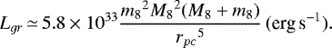 (40)
(40)
For binary systems, the characteristic gravitational wave frequency is twice the Keplerian orbital frequency:
 (41)
(41)
or
 (42)
(42)
When a binary coalesces, gravitational waves will burst due to the merging of the holes. The period and dimensionless amplitude of the gravitational wave burst can be estimated as:
 (43)
(43)
or
 (44)
(44)
and the gravitational wave frequency fgw = 1/Tgw.
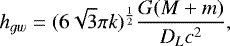 (45)
(45)
or
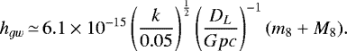 (46)
(46)
Here, k is the emission efficiency of the gravitational radiation. For the massive stellar binary black hole merger GW20150914 observed by LIGO, k ≃ 0.046 (Abbott et al. 2016b).
We list these parameters of gravitational waves for 1302-102 in Table 5, which are derived using the specific model parameters from Table 4 for four inclination angles.
As shown in the previous section (Table 4) that 1302-102 could be a supermassive black hole binary with a hole separation of ~0.02 pc and has started to enter the inspiral phase with the energy-momentum loss by gravitational radiation dominating the shrinkage of the orbit before ultimate merging (Haehnelt 1994; Volonteri et al. 2003). But as shown in Table 5, its characteristic gravitational wave frequencies are in the range of 10−8–10−6 Hz which are inorders of magnitude lower than the lower limit of the currently planned gravitational wave detectors (e.g., eLISA; Jafry et al. 1994; Artymowicz 1998; Bender 1998, Bender & Dieter 2003; Komossa 2003; Merritt 2003; Milosavljevic & Merritt 2003; Merritt & Milosavljevic 2005; Amaro-Seoane et al. 2013; Farris et al. 2014; Bogdanovic 2015). Thus, in the binary hole scenario of large inclinations QSO 1302-102 may not be an appropriate candidate for the gravitational wave experiments currently planned. However, the recent discovery of the gravitational-wave source GW150914 with the Advanced LIGO detectors (e.g., Abbott et al. 2016a, b, c, d; Castelvecchi 2016) demonstrates the very bright future of detections of gravitational waves in extragalactic supermassive black hole binaries, including some blazars with very short precession period.
Recently, Valtonen et al. (2016) observed the predicted optical outburst in OJ287 occurred in November–December 2015, which is clearly separated into the thermal bremsstrahlung and synchrotron components, solving the key issue on the radiation mechanisms of the optical outbursts (Qian 2015). This confirms the applicability of their binary black hole model and implies that in the case of OJ287, evidence for gravitational radiation during the inspiral phase can be inferred from the modeling of the orbital precession and timing of the quasi-periodic optical outbursts (Valtonen et al. 2006, 2008).
Parameters of gravitational radiation for 1302-102.
6 Conclusions
We have investigated the kinematics of QSO PG 1302-102 and obtained the following results.
Based on the analysis of the ejection epochs of the VLBI features we find that the radio jet has a precession period of ~ 5.1583 ± 0.5 yr, periodically ejecting superluminal components. This period is derived completely from the radio observations;
The kinematics of all the six components can be consistently and well fitted in terms of the precessing nozzle model (or precessing common trajectory model) originally proposed by Qian et al. (1991). Their inner trajectories consistently follow the model precessing common trajectory;
The precession period of the radio jet is found to be similar to that of optical variability found in its optical light curve (Graham et al. 2015; D’Orazio et al. 2015). This correlation seems significant for understanding the nature of the optical variability and indicates the importance of the radio jet precession for the optical variations observed in 1302-102;
We assume that 1302-102 harbors a putative supermassive black hole binary in its center. Under the case of large inclinations, we have interpreted both the periodic radio jet swing and the periodic optical variability in terms of the orbital motion of the supermassive black hole binary: the periodic ejection position angle swing is originated from the orbital motion of the primary hole and the periodic optical variability is caused by the orbital motion of the secondary hole (D’Orazio et al. 2015). In this case, the total mass and mass-ratio of the binary and its gravitational radiation can be estimated.
We point out that the finding of the possible relation between the radio jet precession (during 1995–2012) and the periodic optical variability (during 1995-2012) seems favorable for the suggestion that both are caused by the orbital motion of a black hole binary. But the black hole binary model suggested here is tentative and not unique. Further investigations are needed to understand this phenomenon.
The existence of the periodicity in the optical light curve observed in QSO 1032-102 is yet in debate (see Vaughan et al. 2016). Even if the periodic optical variability were due to a red noise process, our model fitting results of the source kinematics and the derived radio jet precession period are not affected, because they are obtained completely from the analyses of the radio observations, without any assumption about the process from which the optical variability originates.
Acknowledgements
We wish to thank Jing-Zhi Zhao (National Astronomical observatories of Chinese Academy of Sciences) for her long lasting help with the preparation of our papers. We have used the MOJAVE database to model the VLBI-maps of 1302-102. The database is maintained by the MOJAVE team (Lister et al. 2009).
References
- Abraham, Z., & Romero, G. E. 1999, A&A, 344, 61 [NASA ADS] [Google Scholar]
- Abbott, B. P., Abbott, R., Abbott, T. D., et al. 2016a, Phys. Rev. D, 93, 122003 [NASA ADS] [CrossRef] [Google Scholar]
- Abbott, B. P., Abbott, R., Abbott, T. D., et al. 2016b, ApJ, 833, L1 [NASA ADS] [CrossRef] [Google Scholar]
- Abbott, B. P., Abbott, R., Abbott, T. D., et al. 2016c, ApJ, 818, L122 [Google Scholar]
- Abbott, B. P., Abbott, R., Abbott, T. D., et al. 2016d, Phys. Rev. Let., 116, 061102 [NASA ADS] [CrossRef] [Google Scholar]
- Agudo, I. 2009, in Approaching Micro-Arcsecond Resolution with VSOP-2: Astrophysics and Technology (ASPCS 402), eds. Y. Hagiwara, E. Fomalont, H. Tsuboi, & Y. Murata (Sagamihara: ISAS/JAXA Institute of Space and Astronomical Science), 330 [Google Scholar]
- Agudo, I., Bach, U., Krichbaum, T. P., et al. 2007, A&A, 476, L17 [NASA ADS] [CrossRef] [EDP Sciences] [Google Scholar]
- Amaro-Seoane, P., & Santamaria, L. 2010, ApJ, 722, 1197 [NASA ADS] [CrossRef] [Google Scholar]
- Amaro-Seoane, P., Aoudia, S., Babak, S., et al. 2013, GW Notes, 6, 4 [Google Scholar]
- Artymowicz, P. 1998, in Theory of Black Hole Accretion Disks, eds. M. A. Abramovicz, G. Bjornsson, & J. E. Pringle (Cambridge, UK: Cambridge University Press), 202 [Google Scholar]
- Asada, K., & Nakamura, M. 2012, ApJ, 745, L28 [NASA ADS] [CrossRef] [Google Scholar]
- Bardeen, J. M., & Petterson, J. A. 1975, ApJ, 195, L65 [NASA ADS] [CrossRef] [Google Scholar]
- Begelman, M. C., Blandford, R. D., & Rees, M. J. 1980a, Nature, 287, 307 [NASA ADS] [CrossRef] [Google Scholar]
- Begelman M. C., Sarazin, C. L., Hatchett, S. P., et al. 1980b, ApJ, 238, 722 [NASA ADS] [CrossRef] [Google Scholar]
- Bender, P. L. 1998, in Eighteenth Texas Symposium on Relativistic Astrophysics and Cosmology, eds. A. V. Olinto, J. A. Frieman, & D. N. Schramm (Singapore: World Scientific), 536 [Google Scholar]
- Bender, P. L., & Dieter, H. 2003, Adv. Space Res., 32, 1243 [NASA ADS] [CrossRef] [Google Scholar]
- Beskin, V. S., & Zheltoukhov, A. A. 2013, Astron. Lett., 39, 215 [NASA ADS] [CrossRef] [Google Scholar]
- Biretta, J. A., Junor, W., & Livio, M. 2002, New Astron., 46, 239 [NASA ADS] [CrossRef] [Google Scholar]
- Bogdanovic, T. 2015, ASSP, 40, 103 [NASA ADS] [CrossRef] [Google Scholar]
- Britzen, S., Roland, J., Laskar, J., et al. 2001, A&A, 374, 784 [Google Scholar]
- Britzen, S., Qian, S. J., Steffen, W., et al. 2017, A&A, 602, A29 [NASA ADS] [CrossRef] [EDP Sciences] [Google Scholar]
- Calzadilla, M., Fish, V. L., Lu, R., et al. 2015, AAS Meeting, 225, 432.11 [Google Scholar]
- Caproni, A., & Abraham, Z. 2004a, ApJ, 602, 625 [NASA ADS] [CrossRef] [Google Scholar]
- Caproni, A., Cuesta, H. J. M., & Abraham, Z. 2004b, ApJ, 616, L99 [NASA ADS] [CrossRef] [Google Scholar]
- Caproni, A., Livio, M., Abraham, Z., & Cuesta, H. J. M. 2006, ApJ, 653, 112 [NASA ADS] [CrossRef] [Google Scholar]
- Castelvecchi, D. 2016, Nature, 530, 261 [NASA ADS] [CrossRef] [Google Scholar]
- Charisi, M., Bartos, I., Haiman, Z., et al. 2015, MNRAS, 454, L21 [NASA ADS] [CrossRef] [Google Scholar]
- Daly, R. A., & Marscher, A. P. 1988, ApJ, 334, 539 [NASA ADS] [CrossRef] [Google Scholar]
- Doeleman, S. S., Fish, V. L., Schenck, D. E., et al. 2012, Science, 338, 355 [NASA ADS] [CrossRef] [PubMed] [Google Scholar]
- D’Orazio, D. J., Haiman, Z., MacFadyen, A. 2013, MNRAS, 436, 2997 [NASA ADS] [CrossRef] [Google Scholar]
- D’Orazio, D. L., Haiman, Z., Schminovich, D. 2015, Nature, 525, 351 [NASA ADS] [CrossRef] [Google Scholar]
- Einstein, A. 1916, Sitzungberichte der Königlich Preussischen Akademie der Wissenschafte (Berlin: SPAW), 688 [Google Scholar]
- Einstein, A. 1918, Sitzungberichte der Königlich Preussischen Akademie der Wissenschafte (Berlin: SPAW), 154 [Google Scholar]
- Farris, B. D., Duffell, P., MacFadyen, A. I., et al. 2014, ApJ, 783, 134 [NASA ADS] [CrossRef] [Google Scholar]
- Fukushige, T., & Ebisuzaki, T. 1992, ApJ, 396, L61 [NASA ADS] [CrossRef] [Google Scholar]
- Gaskell, C. M. 1985, Nature, 315, 386 [NASA ADS] [CrossRef] [Google Scholar]
- Gebhardt, K., Adams, J., Richstone, D., et al., 2011, ApJ, 729, 119 [NASA ADS] [CrossRef] [Google Scholar]
- Gergely, L. A., & Biermann, P. L. 2009, ApJ, 697, 1261 [NASA ADS] [CrossRef] [Google Scholar]
- Graham, M. J., Djorgovski, S. G., Stern, D., et al. 2015, Nature, 518, 74 [NASA ADS] [CrossRef] [Google Scholar]
- Haehnelt, M. G. 1994, in Multi-Wavelength Continuum Emission of AGN, eds. T. J.-L. Courvoisier, & A. Blecha (Dordrecht: Kluwer Academic), 279 [CrossRef] [Google Scholar]
- Hogg, D. W. 1999, ArXiv e-prints [arXiv:9905116] [Google Scholar]
- Homan, D. C., Ojha, R., Wardle, J. F. C., et al. 2001, ApJ, 549, 840 [NASA ADS] [CrossRef] [Google Scholar]
- Homan, D. C., Kadler, M., Kellermann, K. I., et al., 2009, ApJ, 706, 1253 [NASA ADS] [CrossRef] [Google Scholar]
- Homan, D. C., Lister, M. L., Kovalev, Y. Y., et al. 2015, ApJ, 798, 134 [Google Scholar]
- Hutchings, J. B., Morris, S. C., & Gower, A. C., et al. 1994, PASP, 106, 642 [NASA ADS] [CrossRef] [Google Scholar]
- Jackson, N., O’Brien, P. T., Goad, M., et al. 1992, A&A, 262, 17 [NASA ADS] [Google Scholar]
- Jafry, Y. R., Cornelisse, J., & Reinhard, R. 1994, ESA J., 18, 219 [NASA ADS] [Google Scholar]
- Katz, J. I. 1997, ApJ, 478, 527 [NASA ADS] [CrossRef] [Google Scholar]
- Kikuchi, S., Inoue, M., Mikami, Y., et al. 1988, A&A, 190, L8 [NASA ADS] [Google Scholar]
- Kokkotas, K. D., & Schmidt, B. G. 1999, Liv. Rev. Rel., 2, 72 [Google Scholar]
- Komossa, S. 2003, in The Astrophysics of Gravitational Wave Sources, ed. J. Centrella, AIPC, 686, 161 [Google Scholar]
- Kudrayavtseva, N. A., Britzen, S., Witzel, A., et al. 2011, A&A, 526, A51 [NASA ADS] [CrossRef] [EDP Sciences] [Google Scholar]
- Kun, E., Frey, S., Gabányi, K.É., et al. 2015, MNRAS, 454, 1290 [NASA ADS] [CrossRef] [Google Scholar]
- Lang, K. R. 2002, Astrophysical Formulae, Vol. 2: Space, Time, Matter and Cosmology (New York: Springer) [Google Scholar]
- Lense, J., & Thirring H., 1918, Phys. Z. 19, 156 [Google Scholar]
- Lister, M. L., Cohen, M.H., Homan, D. C., et al., 2009, AJ, 138, 3718 [NASA ADS] [CrossRef] [Google Scholar]
- Lister, M. L., Aller, M. F., Aller, H. D., et al. 2013, AJ, 146, 120 [NASA ADS] [CrossRef] [Google Scholar]
- Liu, S., & Melia, F. 2002, ApJ, 573, L23 [NASA ADS] [CrossRef] [Google Scholar]
- Lobanov, A. P., & Roland, J. 2005, A&A, 431, 831 [NASA ADS] [CrossRef] [EDP Sciences] [Google Scholar]
- Lu, J. F. 1990, A&A, 229, 424 [NASA ADS] [Google Scholar]
- Marziani, P., Sulentic, J. W., Dultzin-Hacyan, D., et al. 1996, ApJS, 104, 37 [Google Scholar]
- McKinney, J. C., Tchekhovskoy, A., & Blandford, R. D. 2012, MNRAS, 423, 2083 [NASA ADS] [CrossRef] [Google Scholar]
- Merritt, D. 2003, in Coevolution of Black Holes and Galaxies, ed. L. C. Ho (Cambridge, UK: Cambridge University Press), 263 [Google Scholar]
- Merritt, D., & Milosavljevic, M. 2005, Liv. Rev. Rel., 8 [Google Scholar]
- Milosavljevic, M., & Merritt, D. 2003, AIPC, 686, 201 [NASA ADS] [Google Scholar]
- Misner, C. M., Thorne, K. S., & Wheeler, J. A. 1973, Gravitation (san Fransisco: Freeman) [Google Scholar]
- Mohan, P., An, T., Frey, S., et al. 2016, MNRAS, 463, 1812 [NASA ADS] [CrossRef] [Google Scholar]
- Molina, S. N., Agudo, I., & Gómez, J. L. 2014, A&A, 566, A26 [NASA ADS] [CrossRef] [EDP Sciences] [Google Scholar]
- Nakamura, M., & Asada, K. 2013, ApJ, 775, 118 [NASA ADS] [CrossRef] [Google Scholar]
- Narayan, R., McClintock, J.E., & Tchekhovskoy, A. 2014, in General Relativity, Cosmology and Astrophysics, Fundamental theories of Physics (Switzerland: Springer International Publishing), 177, 523 [NASA ADS] [Google Scholar]
- Nelson, R. P., & Papaloizou, J. C. B. 2000, MNRAS, 315, 570 [NASA ADS] [CrossRef] [Google Scholar]
- Pen, Ue-Li 1999, ApJS, 120, 49 [NASA ADS] [CrossRef] [Google Scholar]
- Peters, P. C. 1964, Phy. Rev., 136, 1224 [Google Scholar]
- Punsly, B. 2001, Black Hole Gravitohydromagnetics (New York: Springer) [CrossRef] [Google Scholar]
- Qian, S. J. 2011, Res. Astron. Astrophys., 11, 43 [NASA ADS] [CrossRef] [Google Scholar]
- Qian, S. J. 2012, Res. Astron. Astrophys., 12, 46 [NASA ADS] [CrossRef] [Google Scholar]
- Qian, S. J. 2013, Res. Astron. Astrophys., 13, 783 [NASA ADS] [CrossRef] [Google Scholar]
- Qian, S. J. 2015, Res. Astron. Astrophys., 15, 287 [Google Scholar]
- Qian, S. J. 2016, Res. Astron. Astrophys., 16, 20 [NASA ADS] [CrossRef] [Google Scholar]
- Qian, S. J., Witzel, A., Krichbaum, T., et al. 1991, Acta Astron. Sin., 32, 369 (english translation: in Chin. Astro. Astrophys., 16, 137 (1992)) [Google Scholar]
- Qian, S. J., Kudryavtseva, N. A., Britzen, S., et al. 2007, Chinese J. Astron. Astrophy., 7, 364 [NASA ADS] [CrossRef] [Google Scholar]
- Qian, S. J., Witzel, A., Zensus, J. A., et al. 2009, Res. Astron. Astrophys., 9, 137 [NASA ADS] [CrossRef] [Google Scholar]
- Qian, S. J., Britzen, S., Witzel, A., et al. 2014, Res. Astron. Astrophys., 14, 249 [NASA ADS] [CrossRef] [Google Scholar]
- Qian, S. J., Britzen, S., Witzel, A., et al. 2017, A&A, 604, A90 [NASA ADS] [CrossRef] [EDP Sciences] [Google Scholar]
- Raiteri, C. M., Villata, M., Aller, H. D., et al. 2001, A&A, 377, 396 [NASA ADS] [CrossRef] [EDP Sciences] [Google Scholar]
- Roland, J., Britzen, S., Caproni, A., et al. 2013, A&A, 557, A85 [Google Scholar]
- Roland, J., Britzen, S., Kun, E., et al. 2015, A&A, 578, A86 [NASA ADS] [CrossRef] [EDP Sciences] [Google Scholar]
- Roos, N., Kaastra, J. S., & Hummel, C. A. 1993, ApJ, 409, 130 [NASA ADS] [CrossRef] [Google Scholar]
- Sarazin, C. L., Begelman, M. C., & Hatchett, S. P. 1980, ApJ, 238, L129 [NASA ADS] [CrossRef] [Google Scholar]
- Savolainen, T., Wiik, K., Valtaoja, E., & Tornikoski, M. 2006, A&A, 446, 71 [NASA ADS] [CrossRef] [EDP Sciences] [Google Scholar]
- Scheuer, P. A. G. 1992, in Extragalactic Radio Sources: From Beams to Jets, eds. J. Roland, H. Sol, & G. Pelletier (Cambridge, UK: Cambridge University Press), 368 [Google Scholar]
- Scheuer, P. A. G., & Feiler, R. 1996, MNRAS, 282, 291 [NASA ADS] [CrossRef] [Google Scholar]
- Shapiro, S. L., & Teukolsky S. A. 1983, Black Holes, White Dwarfs, and Neutron Stars: The Physics of Compact Objects (New York: Wiley-Interscience) [Google Scholar]
- Shi, J. M., & Krolik, J. H. 2015, ApJ, 807, 131 [NASA ADS] [CrossRef] [Google Scholar]
- Shi, J. M., Krolik, J. M., Lubow, S. H., Hawley, J. F. 2012, ApJ, 749, 118 [NASA ADS] [CrossRef] [Google Scholar]
- Sillanpää, A., Haarala, S., Valtonen, M. J., et al. 1988, ApJ, 325, 628 [NASA ADS] [CrossRef] [Google Scholar]
- Spergel, D. N., Verde, L., Peiris, H. V., et al. 2003, APJS, 148, 175 [NASA ADS] [CrossRef] [Google Scholar]
- Steffen, W., Zensus, J. A., Krichbaum, T. P., et al. 1995, A&A, 302, 335 [Google Scholar]
- Stirling, A. M., Cawthorne, T. V., Stevens, J. A., et al. 2003, MNRAS, 341, 405 [NASA ADS] [CrossRef] [Google Scholar]
- Sudou, H., Iguchi, S., Murata, Y., & Taniguchi, Y. 2003, Science, 300, 1263 [NASA ADS] [CrossRef] [Google Scholar]
- Tateyama, C. E. 2009, ApJ, 705, 877 [NASA ADS] [CrossRef] [Google Scholar]
- Tateyama, C. E. 2013, ApJS, 205, 15 [NASA ADS] [CrossRef] [Google Scholar]
- Tateyama, C. E., & Kingham, K. A. 2004, ApJ, 608, 149 [NASA ADS] [CrossRef] [Google Scholar]
- Thorne, K. S., & Braginsky, V. B. 1976, ApJ, 204, L1 [NASA ADS] [CrossRef] [Google Scholar]
- Thorne, K. S., & Blandford, R. D. 1982, in Extragalactic Radio Sources, eds. D. S. Heeschen, & C. M. Wade (Dordrecht: D. Reidel Publishing), Proc. IAU Symp. 255 [Google Scholar]
- Valtonen, M., & Wiik, K. 2012, MNRAS, 421, 1861 [NASA ADS] [CrossRef] [Google Scholar]
- Valtonen, M., & Pihajoki, P. 2013, A&A, 557, A28 [NASA ADS] [CrossRef] [EDP Sciences] [Google Scholar]
- Valtonen, M. J., Lehto, H. J., Sillanpää, A., et al. 2006, ApJ, 646, 36 [NASA ADS] [CrossRef] [Google Scholar]
- Valtonen, M. J., Lehto, H. J., Nilsson, K., et al. 2008, Nature, 452, 851 [NASA ADS] [CrossRef] [PubMed] [Google Scholar]
- Valtonen, M. J., Zola, S., Ciprini, S., et al. 2016, ApJ, 819, L37 [NASA ADS] [CrossRef] [Google Scholar]
- Vaughan, S., Uttley, P., Markowitz, A. G., et al. 2016, MNRAS, 461, 3145 [NASA ADS] [CrossRef] [Google Scholar]
- Villata, M., Raiteri, C. M., Sillanpää, A., & Takalo, L. O. 1998, MNRAS, 293, L13 [NASA ADS] [CrossRef] [Google Scholar]
- Vlahakis, N., & Koenigl, A. 2004, ApJ, 605, 656 [NASA ADS] [CrossRef] [Google Scholar]
- Volonteri, M., Haardt, F., & Madau, P. 2003, ApJ, 582, 559 [NASA ADS] [CrossRef] [Google Scholar]
This value is smaller than that (5° ± 0.2°) given by Graham et al. (2015).
VLBI maps have been made by using the MOJAVE database (Kun et al. 2015), which is maintained by the MOJAVE team (Lister et al. 2009).
These parameters and the trajectory patterns of the knots are all defined in the (X, Y, Z) system. Thus the variations in these parameters imply the changes of the trajectory patterns with respect to the observer system (Xn, Yn, Zn).
In this paper the observed curvatures in the outer trajectories are interpreted in terms of the changes in parameter ψ. Alternative explanations are possible, for example, by using the changes in trajectory amplitude A(Z), see Qian et al. (2017).
The three data-points observed at 1998.84, 1999.55 and 2001.99 can not be well fitted and could be due to another feature or VLBI-modeling defects (e.g., Homan et al. 2001).
Since in the case of PG 1302-102 the viewing angle of the jet axis is very small (ϵ = 1.5°), for simplicity we will ignore the difference between the direction of the jet axis and the direction toward the observer.
We would suggest to add an optical jet component associated with the radio jet, but in the case of cavity-accretion its emission may be negligible relative to these disk emissions.
As in the prominent binary black hole candidate OJ287 (Valtonen & Pihajoki 2013) we assume that the secondary hole does not produce a jet.
All Tables
Parameters selected for the precessing nozzle model for modeling the inner trajectories and kinematics.
Core separations rn (mas) and thecorresponding distance Z (mas and pc) along the precession axis within which the inner trajectories of the knots are well fitted in terms of the precessing nozzle model with a precession period of ~5.16 yr.
All Figures
|
Fig. 1 Geometry of the precessing jet nozzle model adopted from Qian (2011). Three coordinate systems are used: (Xn, Yn, Zn), (X, Y, Z) and (Xp, Yp, Zp). The Yn axis is directed toward the observer and the Xn–Zn plane represents the sky plane. The (X, Y, Z) system is defined with respect to the (Xn,Yn,Zn) system and the precession axis (Z-axis) is defined by parameters (ϵ, ψ). The trajectory of a knot (superluminal component) is defined by parameters (A(Z), Φ) in the (X, Y, Z) system. θ denotes the angle between the knot’s velocity vector S and the direction toward the observer V; η is the initialhalf opening angle of the jet. (see text). |
| In the text | |
|
Fig. 2 Amplitude function A(Z) and precession phase Φ(Z) for describing the trajectory of knot C1. Its entire trajectory observed and kinematics can be well modeled in terms of the precessing nozzle model. |
| In the text | |
|
Fig. 3 KnotsC1 and C6 have almost equal position angles and move along very similar trajectories, but their observed ejection times are 1991.58 ± 0.28 and 2007.31 ± 0.30, differing by 15.73 yr. If this similarity of the position angles at the two ejection epoches is caused by the jet precession, then its is argued that 15.73/3 = 5.24 yr is the most appropriate precession period. The dotted and dashed lines denote the modeledtrajectories for knots C1 and C6, respectively (see text). |
| In the text | |
|
Fig. 4 Upper panel: modeled distribution of the trajectory of the precessing nozzle model for the inner jet regions. ϕ = 1.0, 2.0, 3.0, 4.0, 5.0, and 6.0 rad. The common trajectory rotates around the precession axis anticlockwise viewed along the axis. The precession axis is at position angle of 30.1°. Middle panel: distribution of the observed trajectories of knots C1–C6 in the plane of the sky. Bottom panel: model fitting of the core separations for knots C1–C6. The model fitting of their kinematics are shown individually in Figs. 5–10. |
| In the text | |
|
Fig. 5 Model fitting results of the kinematics for knot C1. It moves along the modeled precessing common trajectory during the whole observation period (core separation rn < 2 mas). In the upper right panel two additional modeled trajectories (green and magneta lines) calculated for the modeled ejection epoches t0 ± 0.5 yr (or ϕ ± 0.61 rad) are also shown, demonstrating that most of the observation data points are within the position angle range defined by the two additional modeled trajectories and the precession period is determined within an uncertainty of ~ ± 0.5 yr. |
| In the text | |
|
Fig. 6 Model fitting results of the kinematics for knot C2. Within core separation rn < 1.47 mas, ψ = constant = − 2.097 and knot C2 moves along the modeled precessing common trajectory. In the upper left panel the dashed red line (modeling the entire trajectory) and the solid black line (modeling the inner trajectory) coincide within core separation rn < 1.47 mas, showing a small curvature in its outer trajectory. In the upper right panel two additional modeled trajectories calculated for t0 ± 0.5 yr (or ϕ ± 0.61 rad) are added todemonstrate that most of the observation data points are within the position angle range defined by the two additional modeled trajectories (green and magneta lines) and the precession period is determined within an uncertainty of ~ ± 0.5 yr. |
| In the text | |
|
Fig. 7 Results of the model fitting of the kinematics for knot C3. Within core separation rn < 1.19 mas its inner trajectory follows the precessing common trajectory. In the upper left panel the red dashed line (modeling the entire trajectory) and the solid black line (modeling the inner trajectory) coincide within core separation rn < 1.19 mas, showing the curvature in its outer trajectory. In the upper right panel two additional modeled trajectories (green and magneta lines) for ejection epoches t0 ± 0.5 yr (or ϕ ± 0.61 rad) are also added, demonstrating that most of the observation data points are within the position angle range defined by the two additional modeled trajectories and the precession period is determined within an uncertainty of ~ ± 0.5 yr. |
| In the text | |
|
Fig. 8 Modeling results of the kinematics for knot C4. It moves along a curved trajectory with small oscillations. Its inner trajectory and kinematics can be well fitted by the precessing nozzle model within core separation rn < 0.58 mas. In the upper left panel the solid black line (modeling the inner trajectory) and the dashed red line (modeling the entire trajectory) coincide within core separation of 0.58 mas, showing the curvatures in its outer trajectory. In the upper right panel two additional modeled trajectories are shown for ejection epochs t0 ± 0.5 yr, demonstrating that most of the observation data points are within the position angle range defined by the two trajectories (green and magneta lines) and the precession period is determined within an uncertainty of ~ ± 0.5 yr. |
| In the text | |
|
Fig. 9 Modeling results of the kinematics for knot C5. It moves along a curved trajectory and the data points from Lister et al. (2009 for knot C6, designated as LC6 here) are added to check its initial trajectory pattern. In the upper left panel the dashed red line (modeling the entire trajectory) and the solid black line (modeling the inner trajectory) coincide within core separation rn < 1.04 mas, evidently showing the transition from the precession common trajectory to the curved trajectory in the outer jet region. In the upper right panel two additional modeled trajectories calculated for ejection epoches t0 ± 0.5 yr (or ϕ ± 0.61 rad), demonstrating that most of the observation data points are within the position angle range defined by the two additional modeled trajectories (green and magneta lines) and the precession period is determined within an uncertainty of ~ ± 0.5 yr. |
| In the text | |
|
Fig. 10 Model fitting results for knot C6. Knot C6 moves along the precessing common trajectory during the whole observation period. In the upper left panel the solid black line (modeling the inner trajectory) and the dashed red line (modeling the entire trajectory) coincide. In the upper right panel three modeled trajectoryies are shown for t0 (black dashed line) and t0 ± 0.5 yr (or ϕ ± 0.61 rad; green and magneta lines), demonstrating that most of the observation data points are within the position angle range defined by the two additional modeled trajectories and the precession period is determined within an uncertainty of ~ ± 0.5 yr. |
| In the text | |
|
Fig. 11 Some relations for the inner precessing nozzle model. Top panel: modeled relation between the ejection position angle and the initial viewing angle, denoting the PA range of ~ 20° (from 20° to 40°) and the viewing angle range of ~ 0.54° (from 1.23° to 1.77°). The precession axis is at (30.14°, 1.50°). Middle panel: Modeled PA(t) and the modeled position angles of knots C1–C6. Lower panel: flux density variations of the VLBI-core and the total source at 15 GHz and the Doppler beaming ratio
|
| In the text | |
Current usage metrics show cumulative count of Article Views (full-text article views including HTML views, PDF and ePub downloads, according to the available data) and Abstracts Views on Vision4Press platform.
Data correspond to usage on the plateform after 2015. The current usage metrics is available 48-96 hours after online publication and is updated daily on week days.
Initial download of the metrics may take a while.