| Issue |
A&A
Volume 615, July 2018
|
|
|---|---|---|
| Article Number | A169 | |
| Number of page(s) | 10 | |
| Section | Astrophysical processes | |
| DOI | https://doi.org/10.1051/0004-6361/201731710 | |
| Published online | 07 August 2018 | |
Non-resonant Alfvénic instability activated by high temperature of ion beams in compensated-current astrophysical plasmas
1
Main Astronomical Observatory, NASU, Kyiv, Ukraine
e-mail: This email address is being protected from spambots. You need JavaScript enabled to view it.
2
Solar-Terrestrial Centre of Excellence, Royal Belgian Institute for Space Aeronomy, Ringlaan 3, 1180 Brussels, Belgium
e-mail: This email address is being protected from spambots. You need JavaScript enabled to view it.
Received:
3
August
2017
Accepted:
23
April
2018
Abstract
Context. Compensated-current systems are established in response to hot ion beams in terrestrial foreshock regions, around supernova remnants, and in other space and astrophysical plasmas.
Aims. We study a non-resonant reactive instability of Alfvén waves propagating quasi-parallel to the background magnetic field B0 in such systems.
Methods. The instability is investigated analytically in the framework of kinetic theory applied to the hydrogen plasmas penetrated by hot proton beams.
Results. The instability arises at parallel wavenumbers kz that are sufficiently large to demagnetize the beam ions, kzVTb/ωBi ≳ 1 (here VTb is the beam thermal speed along B0 and ωBi is the ion-cyclotron frequency). The Alfvén mode is then made unstable by the imbalance of perturbed currents carried by the magnetized background electrons and partially demagnetized beam ions. The destabilizing effects of the beam temperature and the temperature dependence of the instability threshold and growth rate are demonstrated for the first time. The beam temperature, density, and bulk speed are all destabilizing and can be combined in a single destabilizing factor αb triggering the instability at αb > αbthr, where the threshold value varies in a narrow range 2.43 ≤ αbthr ≤ 4.87. New analytical expressions for the instability growth rate and its boundary in the parameter space are obtained and can be directly compared with observations. Two applications to terrestrial foreshocks and foreshocks around supernova remnants are briefly discussed. In particular, our results suggest that the ions reflected by the shocks around supernova remnants can drive stronger instability than the cosmic rays.
Key words: plasmas / waves / instabilities / solar wind / ISM: supernova remnants
© ESO 2018
1. Introduction
Diluted ion beams propagating along the background magnetic field B0 are widespread in space and astrophysical plasmas, including solar wind (Marsch 2006, and references therein), terrestrial foreshocks (Paschmann et al. 1981, and references therein), supernova remnants (Bell 2005, and references therein), and many other astrophysical environments (Zweibel & Everett 2010, and references therein). As the plasmas are typically quasi-neutral, the background electrons tend to follow the beam ions compensating their current. Depending on particular settings, the compensating currents can also be provided by other plasma components, like co-streaming electron beams injected simultaneously with the ion beams. Plasma instabilities developing in such compensated-current systems not only regulate the plasma and beam parameters keeping them close to the marginally unstable states, but can also be important sources for the background plasma heating, energetic particle acceleration, and amplification of the background magnetic field.
Plasma waves in the compensated-current systems can be driven unstable by resonant (Duijveman et al. 1981; Gary 1985; Vojtenko et al. 1990) and non-resonant (Winske & Leroy 1984; Bell 2004; Achterberg 2013) wave–particle interactions. Resonant kinetic instabilities of various wave modes, driven by the beam ions, have been studied extensively in the past. Parallel-propagating Alfv én and fast waves have been found to be strongly unstable for beam velocities higher than a few Alfvén velocities (e.g., Gary 2005; Marsch 2006, and references therein). Concurrent instabilities of oblique (kinetic) Alfvén waves come into play at lower (but still super-Alfvénic) beam velocities (Voitenko 1998).
The above-mentioned instabilities can be driven directly by the beam ions (Sentman et al. 1981; Winske & Leroy 1984; Gary 1985) or by the electron return currents (Winske & Leroy 1984; Bell 2004; Chen & Wu 2012, and references therein). The non-compensated electron currents flowing along B0, may also drive both the resonant (Voitenko 1995) and non-resonant (Malovichko & Iukhimuk 1992; Malovichko 2007) instabilities of Alfvén waves. The simplest case of purely parallel propagating Alfvén waves has been considered in application to the current-carrying coronal loops (Malovichko & Iukhimuk 1992), where these waves appeared to always be unstable. Later on, the analysis was extended by accounting for the oblique propagation (Malovichko 2007) and the currents curried by low-density beams (Malovichko 2010), and applied to the terrestrial magnetosphere and coronal loops.
Self-consistent modifications of the background magnetic field by the electric currents, neglected by Malovichko & Iukhimuk (1992), Malovichko (2007); and Voitenko (1995), may reduce or even stabilize current instabilities. This issue does not concern instabilities developing in compensated-current systems. Such systems, formed around supernova remnants by high-energy streaming cosmic rays (CRs), were studied by Bell (2004), who found a new non-resonant Alfvénic instability (hereafter Bell instability). Since then, the Bell instability and its modifications have attracted a lot of interest (see, e.g., Amato & Blasi 2009; Bret 2009; Zweibel & Everett 2010; Schure et al. 2012; Achterberg 2013; Kobzar et al. 2017, and references therein). Following Bell (2004), the primary focus was on the unstable modes with finite kzV̄bz/ωBi propagating along B0 (where V̄bz is a characteristic velocity of the beam ions along the mean magnetic field B0 || z; kz is the parallel wavenumber; and ωBi is the ion-cyclotron frequency). Compensated currents can also drive an oblique Alfvén instability (Malovichko et al. 2014) for which the perpendicular wave dispersion due to finite k⊥VTb⊥/ωBi is essential (k⊥ and VTb⊥ are the perpendicular wavenumber and beam thermal velocity in the plane ⊥ B0).
Other electrostatic and electromagnetic instabilities may develop in compensated-current systems (see, e.g., Gary 2005; Bret 2009; Brown et al. 2013; Marcowith et al. 2016, and references therein). Which wave modes grow fastest critically depends on the beam and plasma parameters. In the case of cold diluted proton beams propagating along B0, the electrostatic two-stream and Buneman instabilities are much faster than the electromagnetic Alfvénic instabilities (see, e.g., Fig. 44 in Bret et al. 2010). Nevertheless, as is noted by Bret et al. (2010), these electrostatic instabilities are quickly saturated, and then electromagnetic Alfvénic/Bell instabilities come into play. In the hot beam/plasma systems, where the two-stream/Buneman instabilities cannot develop, the electromagnetic Alfvénic/Bell instabilities dominate.
The Bell instability has a maximum growth rate γBell ≃ 0.5j̄bωBi, where j̄b = nbVb/ (n0VA) is the beam current normalized by the Alfvén current. This maximum is attained at the parallel wavenumber |kzm| VA/ωBi = 0.5j̄b and the perpendicular wavenumber k⊥ = 0. These expressions are exactly the same as for the instability studied earlier by Winske & Leroy (1984) in application to the terrestrial foreshock. The difference is that the role of V̄bz in the setting considered by Winske & Leroy (1984) is played by the bulk velocity of the beam Vb rather than the large velocity spread of CRs. Both the Winske–Leroy and Bell instabilities grow fastest when the wave vector k is parallel to B0; they are physically the same instability that can be named the compensated-current parallel instability (CCPI).
The physical mechanism of the CCPI is related to the fact that for sufficiently small parallel wavelengths and sufficiently high V̄bz, the beam protons become partially demagnetized (unfrozen off the perturbed magnetic field). The demagnetization reduces the beam contribution to the fluctuating currents δj ⊥ B0 flowing along the twisted perturbed magnetic field lines, whereas the electron currents remain magnetized, thus providing the non-compensated fluctuating transversal currents. These currents amplify the initial perturbations via the positive feedback loop giving rise to CCPI. This kind of instability is sometimes called reactive.
Surprisingly, despite its importance in astrophysical applications, the CCPI theory is still poorly developed. Many important properties of the instability (the wavenumber dependence of the instability growth rate, behavior of the maximum growth rate in the parameter space, instability boundaries in the parameter spaces, etc.) have not been fully investigated. In the present paper, we study CCPI of Alfvén waves in more detail in the framework of kinetic theory. We consider a simple model of the compensated-current system where the hydrogen plasma is hydrogen plasma is penetrated by the low-density proton beam and the beam current and charge are compensated by the background electrons. Despite its simplicity, this model is applicable to the reactive CCPI driven by compensated currents in many space and astrophysical environments.
2. Plasma model and dispersion equation for Alfvén waves
We consider a three-component plasma consisting of the background steady ion component (i), the low-density ion beam (b) propagating with velocity Vb along z || B0, and the electron component (e) providing the neutralizing current and charge: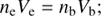 (1)
(1)
 (2)
(2)
We assume here that the beam ions (b) and the background ions (i) are protons. All plasma components are modeled by the shifted Maxwellian velocity distributions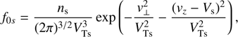 (3)
(3)
where ns, Vs, 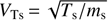 , Ts, and ms are the mean number density, parallel bulk velocity, thermal velocity, temperature, and particle mass of the plasma species s, and v = (vx, vy, vz) – velocity-space coordinates. The subscripts z and ⊥ indicate directions parallel and perpendicular to B0. The plasma model defined by Eqs. ((1)–(3)) has been extensively used in the past (see, e.g., Gary 2005, and references therein). The neutralizing current can also be provided by the co-propagating electron beam (see, e.g., Zweibel & Everett 2010 and references therein); however it does not alter the reactive CCPI for low-density ion beams nb ≪ n0 (Amato & Blasi 2009).
The non-trivial solutions to the Maxwell–Vlasov set of equations exist if the wave frequency ω and the wave vector k = (kx, ky, kz) satisfy the following dispersion equation (see, e.g., Alexandrov et al. 1984)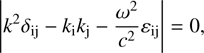 (4)
(4)
where εij is the dielectric tensor and δij is the Kronecker delta. For the parallel-propagating modes with kx = ky = 0, the components of the dielectric tensor given by Alexandrov et al. (1984) reduce to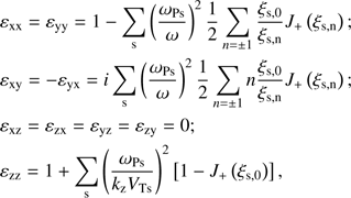 (5)
(5)
where ξs,n = (ω − kzVs + nωBs) / (kzVTs), ωPs (ωBs) is the plasma (cyclotron) frequency. Instead of the plasma dispersion function W (x), we use the function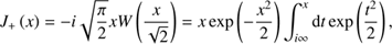 (6)
(6)
introduced by Alexandrov et al. (1984). It has the following asymptotic expansions: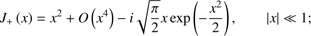 (7)
(7)
and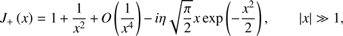 (8)
(8)
where η = 0 for Im x > 0, η = 1 for Im x = 0, and η = 2 for Im x < 0.
In the case of parallel propagation, the dispersion Eq. (4) splits into two independent equations,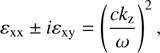 (9)
(9)
describing left-hand (sign −) and right-hand (sign +) polarized electromagnetic waves. In what follows we consider the left-hand polarized Alfvén branch undergoing the compensated-current instability. Taking into account quasi-neutrality (2) and current compensation (1), Eq. (9) for Alfvén waves can be written as (10)
(10)
where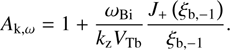
In the following sections we consider important limits of (10) typical for the reactive CCPI instability.
3. Dispersion relation for parallel-propagating waves
As we are going to analyze the reactive non-resonant instability, we neglect the contribution of the imaginary part of J+ (ξb,−1). Furthermore, we consider a low-frequency instability with |ω/ωBi| smaller than other terms in ξb,−1, which allows us to neglect the ω-dependent part in the argument of function J+. In this case (10) reduces to the following quadratic equation with respect to ω/ωBi: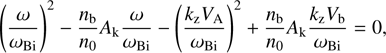 (11)
(11)
where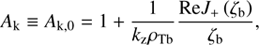 (12)
(12)
ζb = −Vb/VTb − 1/ (kzρTb), and ρTb = VTb/ωBi. To avoid misunderstanding, we note that although ρTb looks like the ion beam gyroradius, it is defined by the parallel beam temperature rather than the perpendicular one, and here it has a different physical meaning.
Equation (11) is the second-order eigenmode equation for Alfvén waves modified by the ion beam and return electron current (second and fourth terms, respectively). Its solution is straightforward: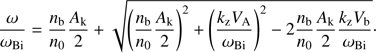 (13)
(13)
From (13) it is obvious that the instability can be driven by the last term under the square root when kzVb > 0. In what follows we assume Vb > 0 considering potentially unstable waves with kz > 0 (in the case of Vb < 0, the identical instability develops for kz < 0 ). In the absence of the beam, Eq. (13) reduces to the Alfvén wave dispersion, ω = kzVA at nb = 0.
The wave with dispersion (13) becomes unstable when the last term under the square root dominates. This term represents effects due to the electron current. The growth rate γ = Im[ω] of the corresponding instability is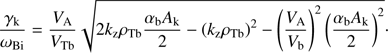 (14)
(14)
Here we introduce the cumulative destabilizing parameter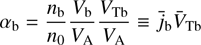 (15)
(15)
that includes all beam parameters. One can think of it as of product of the normalized current j̄b = nbVb/ (n0VA) and velocity spread V̄Tb = VTb/VA of the beam ions. The growth rate (14) is analyzed below analytically and numerically, and its scalings are found in some important limits. It is interesting to note that the right-hand polarized magnetosonic instability can be obtained from the above equation by changing the sign of the first term under the square root (the magnetosonic instability hence requires kzVb < 0).
4. Compensated-current instability driven by hot ion beams
By hot beams we mean the beams whose thermal velocity is significantly larger than the bulk velocity, VTb ≫ Vb. For such beams, the growth rate (14) can be simplified by neglecting the small term Vb/VTb in ξb,−1. The argument of J+ is then simplified to ξb,−1 ≈ −1/ (kzρTb) ≡ ζb. In this case γk depends on the normalized parallel wavenumber kzρTb and two dimensionless bulk parameters, VA/Vb and αb. Then the (maximum) instability growth rate γm = maxkγ appears to be a function of αb and VA/Vb only, whereas the dependence on the general multiplier VA/VTb is trivial and can be excluded by the renormalization of γm. We note that the hot-beam condition VTb > Vb restricts the applicability range of the analytical results obtained below, but in general it does not restrict the instability range (see also Sect. 6).
4.1. Instability areas in the parameter space
Here we find the instability threshold and the instability area in the parameter space (αb, VA/Vb). To this end, we present the growth rate (14) in the following useful form: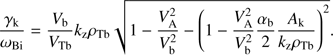 (16)
(16)
From (16), the instability condition is obtained as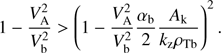 (17)
(17)
Since the right-hand side of (17) is positive, it is obvious that only super-Alfvén beams, Vb > VA, can trigger instability. Therefore, the absolute threshold for the beam velocity is  and the system is stable with respect to reactive CCPI for all Vb < VA.
Using (17), it is also possible to find the threshold for b analytically. First, solving (17) with respect to the kk-dependent term Ak/ (kzρTb), we find that the unstable wavenumbers kz should satisfy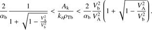 (18)
(18)
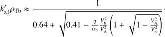
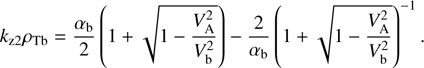
When the velocity threshold is exceeded, Vb > VA, the right boundary of (18) is always larger than the left boundary making the interval between them non-empty. As the function Ak/ (kzρTb) is limited by the maximum value maxk [Ak/ (kzρTb)] ≈ 0.411 achieved at  , the condition (18) can only be satisfied for sufficiently large αb. From the left-hand inequality, it immediately follows the instability condition for αb and the corresponding threshold:
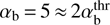
![Mathematical equation: $$ \alpha_\mathrm b>\alpha_\mathrm b^\mathrm{thr}=\frac2{\max_k{\left[\frac{A_\mathrm k}{k_\mathrm z\rho_\mathrm{Tb}}\right]}\left(1+\sqrt{1-\frac{V_\mathrm A^2}{V_\mathrm b^2}}\right)}=\frac{4.866}{1+\sqrt{1-{\left(\frac{V_\mathrm A}{V_\mathrm b}\right)}^2}}. $$](/articles/aa/full_html/2018/07/aa31710-17/aa31710-17-eq25.gif) (19)
(19)
The instability condition  is satisfied above the threshold curve defined by (19), which is shown in Fig. 1 by the solid line. The unstable area above this curve in the parameter space (αb, VA/Vb) is shaded. The dependence of the threshold
  on VA/Vb is rather weak; it grows from the minimum value
  at VA/Vb → 0 to the maximum value
  at VA/Vb → 1. The absolute threshold for αb below which the system is stable is
  . The meaning of the right boundary in (18), shown in Fig. 1 by the dashed line, is clarified in the following subsection.
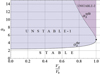 |
Fig. 1. Instability threshold |


In terms of the normalized beam current j̄b = nbVb/ (n0VA) and thermal velocity V̄Tb = VTb/VA, (19) can be written as  . Then the instability condition for the beam thermal velocity reads as
 (20)
(20)
This threshold-like condition is an important new result quantitatively demonstrating the destabilizing effect of the beam temperature. It shows the threshold above which the velocity spread of the beam ions triggers the instability even for weak beams.
Similarly, the threshold condition for the beam current can be written as (21)
(21)
which quantifies the range of unstable beam currents. Again, it is seen that even a weak ion beam can activate CCPI if the beam thermal velocity is sufficiently high. In particular, the beam current required for the instability can be many orders of magnitude smaller than the Alfvén current.
We note that  varies slowly for fast super-Alfv énic beams and can be approximated as
  at Vb/VA > 3. For rough estimations, in all velocity ranges
  can be replaced by its average value 3.5.
4.2. Unstable wavenumber ranges
Properties of CCPI are illustrated further by Figs. 2 and 3 showing all three terms of the condition (18): the left and right boundaries, and the function (kzρTb)−1Ak. The unstable ranges where (18) is satisfied are shaded. A regular single-peak behavior of the function (kzρTb)−1Ak, as seen in Figs. 2 and 3, allows us to investigate how the unstable wavenumber range evolves with αb.
 |
Fig. 2. Illustration of the condition (18) for VA/Vb = 0.9 and αb = 6. In this case |

 |
Fig. 3. Illustration of the condition (18) for VA/Vb = 0:9 and αb = 10. In this case |

When αb increases but is still smaller than  , the left boundary of (18) decreases remaining above the maximum of (kzρTb)−1Ak. In this case there are no unstable wavenumbers and the system is stable. Once αb rises above
  , the decreasing left boundary of (18 ) drops below the maximum of (kzρTb)−1Ak and the unstable wavenumber range kz1 < kz < kz2 appears, where kz1 and kz2 are the lower and upper roots of the equation
 (22)
(22)
As long as αb is not far from the threshold  , there is a single unstable wavenumber interval surrounding
  . This situation is illustrated in Fig. 2, where VA/Vb = 0.9,
  , and
, and  . However, when αb increases further, the right boundary of (18) also drops below the maximum of (kzρTb)−1Ak, which happens at
 (23)
(23)
In this case, shown in Fig. 3 for αb = 9, the right-hand side inequality of (18) is not satisfied in the range  , where
  and
and  are the lower and upper roots of the equation
 (24)
(24)
Instead of unstable, we have now a prohibited wavenumber range around  . As a result, the unstable wavenumber range splits into two: the first unstable range is
  and the second
  .
.
The split threshold  (23) is shown in Fig. 1 by the dashed line. For parameter values above this line, the instability develops in two wavenumber ranges, as mentioned above. These unstable ranges are shown in Fig. 3 by the shaded areas.
Furthermore, Fig. 4 shows the αb dependence of the unstable wavenumber ranges, where the outer and inner boundaries are respectively defined by the left-hand and right-hand margins of (18). It is seen that below  there is no instability, at
  there is a single unstable range of k
z, and above
there is a single unstable range of k
z, and above  there are two unstable ranges.
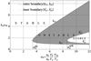 |
Fig. 4. Unstable wavenumber ranges in the (αb, kz) plane for VA/Vb = 0.9. The outer boundary is defined by the left-hand side and the inner boundary by the right-hand side of condition (18). It is seen that below |


From Fig. 3 it is obvious that kz1ρTb and  are located between kzρTb ≈ 0.77, where (kzρTb)−1Ak is zero, and
  , where (kzρTb)−1Ak is maximum. This wavenumber range corresponds to −1.3 < ζb < −0.65, where ReJ+ (ζb) can be approximated by the liner numerical fit
 (25)
(25)
Using this in (22) and (24), we find kz1 and  as
as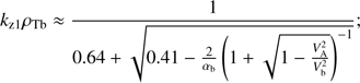 (26)
(26)
 (27)
(27)
From these expressions we see that with increasing αb the difference between kz1 and  decreases,
 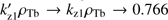 , and the first unstable range becomes very narrow.
On the other hand, the roots kz2ρTb and  bounding the second unstable range, are located above
  , where ζb > −0.65. Then, using the small argument expansion (7) for ReJ+ (ζb), we find
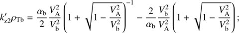 (28)
(28)
 (29)
(29)
At large values of αb, both the width of the second unstable range  and the gap between the unstable ranges
  grow linearly with αb.
In summary, the most important analytical result obtained here is the instability boundary  in the parameter space (VA/Vb; αb), which can be used directly to analyze observational data. The compensated-current systems with VA/Vb < 1 and
  are unstable. The unstable area in the parameter space (VA/Vb; αb) is divided further by
  into two unstable sub-areas:
  with one unstable wavenumber range, and
  with two unstable wavenumber ranges.
4.3. Instability growth rate
Once αb rises above  , an unstable range between kz1 and kz2 appears. The instability growth rate (14) as function of kz is shown in Fig. 5. The plasma parameters αb and VA/Vb in this figure are chosen in such a way as to illustrate the behavior of CCPI in the unstable wavenumber ranges found above. So, the case αb = 6 with one unstable wavenumber range is shown by the dashed line and the case αb = 10 with two unstable wavenumber ranges is shown by the solid lines. The dotted curve in Fig. 5 is for the case αb = 8, which is close to the splitting threshold. It is seen that when the right instability boundary in (18) approaches the maximum of function (kzρTb)−1Ak, the valley and the second peak in γk appear. This happens at
  , where
 (30)
(30)
 |
Fig. 5. Wavenumber dependence of the instability growth rate driven by super-Alfvénic ion beams with VA/Vb = 0.9 for three values of αb: αb = 6, 8, and 10. For larger αb, the unstable area and the maximum growth rate extend to larger kzρTb. |
is the value of αb at which a local “plateau” in γk occurs at the wavenumber where ∂γk/∂kz = 0 and  . For all
  , the secondary peak of γk exists at
  . Since
  , the secondary peak arises before the interval of prohibited wavenumbers
  appears.
It is seen that CCPI is stronger and the most unstable wavenumbers are larger for larger αb. The secondary peak that appears at  is lower than the main peak. These trends are confirmed below analytically.
The most unstable wavenumber and the corresponding maximum growth rate γmax can be found by maximizing (14) with respect to kz, γmax = maxk (γk), which we call the CCPI growth rate. The normalized CCPI growth rate γmax/ωBi as a function of nb/n0 and Vb/VA is shown in Fig. 6 for hot beam with VTb/VA = 102. It is seen that γmax increases rapidly, roughly proportional to both nb/n0 and Vb/VA, which means it is proportional to the current nbVb. This behavior agrees with the current nature of CCPI confirmed below analytically by (34) and (35).
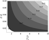 |
Fig. 6. Normalized growth rate γmax/ωBi as a function of nb/n0 and Vb/VA for hot beam with VTb/VA = 102. γmax increases regularly with both nb/n0 and Vb/VA once the threshold is exceeded. |
The threshold for nb/n0 (Vb/VA) is lower for smaller Vb/VA (nb/n0), in agreement with (19). In particular, the velocity threshold  decreases with nb/n0 and reaches the minimum value
  when nbVTb/ (n0VA) → 1.
Dependence of γmax on the thermal velocity VTb is somewhat different (see Fig. 7). First, near the threshold, γmax increases very rapidly with VTb. But this increase quickly slows down as VTb departs further from the threshold. Already at  , γmax becomes virtually independent of VTb.
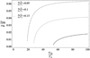 |
Fig. 7. Normalized growth rate γmax/ωBi as a function of VTb/VA for nbVb/ (n0VA) = 0.05 (solid curve), 0.1 (dotted curve), and 0.15 (dashed curve). Starting from zero, the growth rate γmax increases rapidly with VTb, but this increase is quickly saturated. Larger currents nbVb/ (n0VA) result in larger γmax for all VTb. |
To understand this behavior, we proceed with the analytical analysis. Here we take into account that in the wavenumber range  , where the growth rate attains its maximum, the lowζb approximation ReJ+ (ζb) ≈ −(kzρTb)−2 is valid. Thus, using Ak = 1 + ReJ+ (ζb) ≈ 1 − (kzρTb)−2 in (16), we find the following approximation for the maximum of γk:
![Mathematical equation: $$ \frac{\gamma_\max}{\omega_\mathrm{Bi}}\approx\frac12\frac{n_\mathrm bV_\mathrm b}{n_0V_\mathrm A}\sqrt{(1-\frac{V_\mathrm A^2}{V_\mathrm b^2})\left[1-{\left(\frac{\alpha_\mathrm b^\mathrm{thr}}{\alpha_\mathrm b}\right)}^2\right]}. $$](/articles/aa/full_html/2018/07/aa31710-17/aa31710-17-eq96.gif) (31)
(31)
This maximum occurs at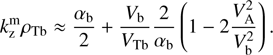 (32)
(32)
The last term in the square parentheses in (31) is adjusted by replacing the approximate numerical value  by
by  to make it compatible with the exact αb threshold (19). We verified numerically that the approximation (31) is good for arbitrary αb, both near the threshold and far from it. In general, with the larger beam velocity and/or temperature, the smaller beam density is needed for instability.
The explicit dependence of the instability growth rate on the beam thermal velocity V̄Tb follows from (31):![Mathematical equation: $$ \frac{\gamma_\max}{\omega_\mathrm{Bi}}\approx\frac{{\overline j}_\mathrm b}2\sqrt{\left(1-\frac1{\overline V_\mathrm b^2}\right)\left[1-{\left(\frac{\alpha_\mathrm b^\mathrm{thr}}{{\overline j}_\mathrm b{\overline V}_\mathrm{Tb}}\right)}^2\right]}. $$](/articles/aa/full_html/2018/07/aa31710-17/aa31710-17-eq100.gif) (33)
(33)
It is seen that γmax increases quickly with V̄Tb once the threshold is overcome,  . The fast increase of γmax reflects the instability response to the progressive demagnetization of the beam ions as their velocity spread increases above the threshold.
However, when V̄Tb becomes large enough, 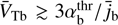 , the term containing it becomes negligibly small and γmax becomes virtually independent of V̄Tb. In this high-temperature regime the beam ions are fully demagnetized and the further increase of V̄Tb no longer affects the instability. This regime corresponds to the asymptotic over-threshold limit
  , where γmax simplifies to
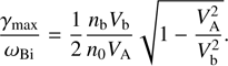 (34)
(34)
The familiar threshold velocity of the beam,  , is still present in (34), but the temperature dependence is already missed, as can be observed in Fig. 7 at large VTb.
The maximum growth rate (34) simplifies further for the fast beams with Vb/VA > 3,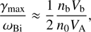 (35)
(35)
with the most unstable parallel wavenumber 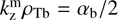 . The asymptotic scaling (35) recovers the scaling obtained by Bell (2004). As is seen from Fig. 7, expressions (34) and (35) provide good estimations for γ
max at
. The asymptotic scaling (35) recovers the scaling obtained by Bell (2004). As is seen from Fig. 7, expressions (34) and (35) provide good estimations for γ
max at 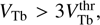 , which also quantifies the meaning of “asymptotic regime” in terms of VTb. It appears that the expressions found by Bell are only valid in this asymptotic regime.
For  , the secondary peak arises at kzρTb < 1.54, where we can use approximation (25). Then for this peak we obtain the local maximum
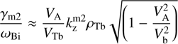 (36)
(36)
attained at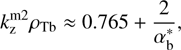 (37)
(37)
where 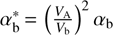 and we took into account that
  . The ratio of this peak to the main peak is
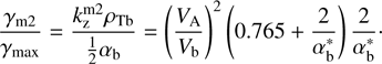 (38)
(38)
Taking into account that 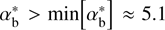 (at VA/Vb → 1), we see that the peak γm2 is always significantly smaller than the main peak γmax. The maximum ratio γm2/ γmax ≈ 0.45 is achieved at
  and VA/Vb ≲ 1.
We note that the unstable fluctuations also have a small oscillatory part Re[ω] = 0.5 (nb/n0) ωBi. For most unstable wavenumber 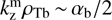 , the real frequency
  is smaller than the frequency of the normal Alfvén mode
  . Since
 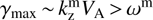 , the instability is aperiodic.
5. Parallel Alfvén instability in particular compensated-current systems
Let us consider two feasible applications of CCPI. First we apply our results to the solar wind upstream of the quasi-parallel terrestrial shock where the plasma conditions are relatively well documented. Then we extend the analysis to the interstellar medium around supernova remnants, assuming the similar scalings of the beam parameters as in the terrestrial foreshock.
5.1. Quasi-parallel terrestrial foreshock
Hot ion beams with VTb > Vb > VA are regularly observed in the solar wind upstream of the terrestrial bow shock where the shock normal is quasi-parallel to the interplanetary magnetic field B0 (Paschmann et al. 1981; Tsurutani & Rodriguez 1981). This ordering of characteristic velocities suggests that CCPI driven by hot ion beams can develop in the quasi-parallel foreshocks.
More specifically, we use the following scalings for characteristic beam velocities, Vb ≲ Vshock and VTb ~ 3Vshock, where the shock velocity is equal to the solar wind speed, Vshock = VSW. These scalings are compatible with observations reported by Paschmann et al. (1981) and Tsurutani & Rodriguez (1981). Yet another beam parameter, number density nb, does not vary much around nb = 0.1 cm−3 (Paschmann et al. 1981). In terms of the background solar-wind density n0 ~ 5–10 cm−3, this gives nb/n0 ~ 0.01–0.02. Taking the typical value of Alfvén velocity, VA ≈ 0.1VSW, we obtain the cumulative destabilizing parameter αb ~ 2.5–5, which is slightly over-threshold depending on the particular value of Vb. Such proximity of the system to the CCPI threshold can be a signature of CCPI operating in the foreshock and relaxing the beam parameters towards the threshold.
On the other hand, as is seen from Fig. 6, even slight deviations of αb from the threshold can make CCPI strong. So, for VA/Vb ~ 0.1 and αb = 6 the maximum growth rate is already high, γmax ≈ 0.07ωBi, with the most unstable wavenumbers kzmρTb ≳ 2. Narita et al. (2006) and Hobara et al. (2007) analyzed properties of electromagnetic fluctuations observed around terrestrial bow shock. Most straightforwardly, our results can be compared with the wavenumber distribution of the fluctuations in the quasi-parallel foreshocks shown in Fig. 9 by Narita et al. (2006), where the measured wavenumbers are normalized by the ion gyroradius. In terms of the background ion gyroradius ρTi, with the typical temperature of the diffuse ions Tb/Ti = 4 × 10², our most unstable wavenumbers kzmρTi ~ kzmρTb/20 ~ 0.1 map upon the major peak observed at kzρTi = 0.1 (see upper panel of Fig. 9 in Narita et al. 2006).
In the quasi-parallel foreshock region, Narita et al. observed another, subdominant peak at kzρTi = 0.6. To explain this peak by CCPI we need a significantly lower beam temperature, Tb/Ti ~ 10, which is more typical for quasi-perpendicular foreshocks. We can speculate that CCPI can also generate this second peak. First, the CCP instability develops in the quasiperpendicular foreshock region where the beams have required temperatures Tb/Ti ~ 10, which is supported by the observed enhancement at kzρTi ≈ 0.4. Then the unstable fluctuations are convected in the quasi-parallel foreshock region where their observed wavenumbers are kzρTi ≈ 0.6.
The above estimations suggest that CCPI can contribute to electromagnetic fluctuations observed in the quasi-parallel terrestrial foreshock and can impose limitations on the parameters of the beams formed by reflected ions. Further direct confrontations of observed values of αb with the stability diagram in Fig. 1 are needed to clarify the role of CCPI in the regulation of ion-beam parameters in the foreshock.
5.2. Foreshock regions around supernova remnants
Supernova remnants expanding in the interstellar medium develop bow shocks at their boundaries. These shocks propagate with high velocities Vshock ~ 2 × 10⁹ cms−1 providing a feasible source of energy for the cosmic ray acceleration, and also for the magnetic field amplification. By analogy with the terrestrial bow shock, we assume that the reflected ions also occur in the supernova foreshocks setting up a compensated-current system. CCPI can develop in supernova foreshocks if parameters of reflected ions (subscript b) satisfy  , defined by (19).
For reasonable background density n0 = 10−2− 1 cm−3 and magnetic field B0 ~ 10−7 − 10−5 G (Zweibel & Everett 2010), the Alfvén velocity varies in the range VA = 2 × 10⁴−2 × 107cm/s. Then the resulting Alfvén Mach number in supernova remnants MA = Vshock/VA = 102−105 is much larger than in Earth’s bow shock. For the similar scalings as in the terrestrial foreshocks, nb/n0 ~ 0.01, Vb ~ 0.5Vshock, and VTb ~ 2Vshock, even with the most unfavorable Vshock/VA = 102 the destabilizing parameter αb ~ 102 is much larger than the threshold  . In this far over-threshold range, the CCPI operates in the asymptotic regime (35) with very high growth rate γmax/ωBi ~ 0.5. We note that this value is already at the edge of applicability of our low-frequency approximation. Such a high growth rate suggests that the instability modifies the beam parameters strongly, in particular reducing the beam velocity towards the local Alfvén velocity, Vb ≳ VA.
Let us compare the instability driven by the reflected ions with the similar instability driven by cosmic rays around supernova remnants (Bell 2004; Zweibel & Everett 2010). Taking the background magnetic field B0 ≳ 10−6 G and the cosmicrays flux nCRVb ~ 104 cm−2 s−1 (Zweibel & Everett 2010), we estimate the normalized current  and the corresponding growth rate
 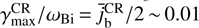 around supernova remnants. With ωBi ≃ 0.03 s−1, we get
 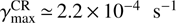 in absolute numbers.
The above estimations show that the CCPI instability driven by reflected ions is much stronger than the instability driven by cosmic rays. Therefore, the former instability can be a more efficient amplifier for magnetic fields around supernova remnants. On the other hand, a fraction of the beam ions can be scattered back to the shock by electromagnetic fluctuations generated by CCPI, thus providing a seed population for the further Fermi acceleration to high cosmic-ray energies.
6. Discussion
A number of competing electrostatic and electromagnetic instabilities may arise when different plasma species move with respect to each other (see Gary 2005; Bret 2009, and references therein). The hierarchical structure of these instabilities depends on many parameters and remains an open question (see further discussions in Bret et al. 2010; Brown et al. 2013; Marcowith et al. 2016).
In our setting with hot ion beams, the fast two-stream/ Buneman instabilities are quenched by the large thermal velocities, which are larger than the streaming velocities. Inspection of Fig. 3.20 by Gary (2005) shows that the thresholds of electrostatic ion-acoustic and ion-cyclotron instabilities are significantly higher than the Alfvénic threshold for VTi/VA ~ Te/Ti ~ 1 typical in the terrestrial foreshock. Among them, the electron/ion cyclotron instability has the lowest threshold velocity, which is still very high,  for nb < 0.1ne. The ion/ion acoustic instability is suppressed further by large beam temperatures, as is seen from Fig. 3.15 by Gary (2005). Therefore, these high-frequency electrostatic instabilities cannot compete with CCPI in the wide range of beam velocities 1 < Vb/VA < 102. At higher beam velocities, Vb/VA > 102, the ion-acoustic and ion-cyclotron harmonic waves can be generated by the electron-ion relative motion. However, even in this velocity range CCPI can develop independently as long as the mean parameters reside in the unstable area (Fig. 1), whereas the kinetic instabilities are quickly saturated by the local quasi-linear plateaus.
Parallel-propagating left-hand and right-hand polarized instabilities have been studied by Gary et al. (1984) and Gary (1985). Using numerical solutions of the dispersion equation, it has been observed that the left-hand polarized Alfvénic instability becomes competitive or even dominant when the beam ions are sufficiently hot (see Fig. 8 by Gary et al. 1984). The condition |ξb,−1| < 1 was used by Gary et al. to categorize this instabilas ion-beam resonant, i.e., resulting from the direct resonant coupling of the unstable mode with the beam ions. However, kinetic and reactive effects have not been distinguished for this mode, which did not allow us to realize that above threshold (19) the instability transforms from kinetic resonant to reactive non-resonant (see Fig. 8 and related discussions below). In the reactive regime, the meaning of the condition |ξb,−1| ≈ |kzρTb|−1 < 1 is reversed: here it indicates that the unstable perturbations are on small enough scales to decouple from the beam ions by the demagnetization effect. The resulting Alfvén instability is then driven not by the resonant interactions with the beam ions, but by the bulk return current of the magnetized electrons. The current nature of this instability is similar to the nature of related current instability (Malovichko & Iukhimuk 1992) that can develop in the absence of any beams.
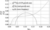 |
Fig. 8. Contribution of the reactive CCPI growth rate (dashed curve) to the total growth rate (dotted curve) for VTi/VA = Te/Ti = 1, Vb/VA = 10, VTb/VA = 25, and nb/n0 = 0.02. It is seen that the reactive destabilizing effects dominate the instability growth rate for this set of parameters. The wave frequency is shown by the solid line. |
Interplay of the reactive and resonant left-hand Alfvénic instabilities also needs further investigations. Our preliminary estimations indicate that the relative importance of the reactive versus kinetic destabilizing effects increases quickly once αb rises above the threshold  . In Fig. 8. we show the contribution of the reactive CCPI to the total growth rate for reference plasma parameters that may occur in foreshocks: VTi/VA = Te/Ti = 1, Vb/VA = 10, VTb/VA = 25, and nb/n0 = 0.02. The corresponding total growth rate in Fig. 8 is given by Eq. (14) with the imaginary part of J+ taken into account. It therefore includes both the reactive effects due to the bulk currents and the resonant wave-particle interactions. It is seen that the destabilizing reactive response becomes stronger than the resonant wave response when αb is still not far from the threshold
  (
( in Fig. 8). The instability is thus driven mainly by the reactive effects and can be analyzed ignoring kinetic resonant effects, as we did in the present study. The same approach can also be applied in the immediate vicinity of the reactive threshold if the quasi-linear plateaus or other local deformations of the velocity distributions weaken destabilizing kinetic effects. Analytical treatment becomes more tangled when reactive and kinetic effects are of comparable efficiency and have to be accounted for simultaneously, in which case the evolution of the system becomes more complex (cf. Yoon & Sarfraz 2017).
There are also left- and right-hand polarized instabilities driven by cold ion beams in the ion-cyclotron frequency range (Mecheri & Marsch 2007). These instabilities are strong when the velocity spread of the beam ions is so small that all the beam ions (and hence the beam as a whole) are resonant. In our settings with hot ion beams these instabilities are quenched similarly to the two-stream/Buneman instabilities.
In the considered case of hot ion beams, Vb/VTb < 1, the analytical treatment of wavenumbers kzρTb < VTb/Vb is simplified by neglecting the term ~Vb/VTb in ξb,−1. As the most unstable wavenumber scales as kzρTb ≈ αb/2 (32), this restriction is not stringent: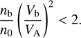 (39)
(39)
This condition is the opposite of the firehose instability condition (see Eq. (14) by Malovichko et al. 2014), which means that the CCPI can operate in a wide range of parameters below the firehose threshold. For cooler beams, where the condition Vb/VTb < 1 is violated (e.g., in the quasi-perpendicular foreshock regions), the analysis should be extended by accounting for corresponding terms.
The compensated-current parallel instability can also affect other processes in space. For example, it can limit the field-aligned currents generated by Alfvén-wave fluxes in the inner magnetosphere and plasma sheet boundary layer (Artemyev et al. 2016). In the solar wind, CCPI can contribute to the regulation of relative motion of different plasma species. It was found that many states of beaming structures in the solar wind are close to the thresholds of magnetosonic and Alfvén instabilities (Marsch & Livi 1987; Gary et al. 2000) and the firehose instability (Chen et al. 2016). Since CCPI can operate close to these thresholds (and sometimes below them), a refined analysis is needed to decide its role in the solar wind, as compared to the magnetosonic and firehose instabilities. These are subjects for future studies.
7. Conclusions
We investigated reactive non-resonant compensated-current parallel instability (CCPI) of left-hand polarized Alfvén waves in compensated-current systems established by hot diluted ion beams. Ion-beam demagnetization due to finite kzρTb is crucial for CCPI (ρTb is based on the parallel beam temperature, and thus does not represent the beam ion gyroradius). New analytical expressions for the instability growth rate (31) and threshold (19) are found and analyzed.
The most important new properties of CCPI can be summarized as follows:
-
Reactive non-resonant CCPI depends on all bulk parameters of the beam: beam density nb, bulk velocity Vb, and thermal velocity VTb. These parameters all increase the instability growth rate and can be combined in the single destabilizing parameter αb = (nb/n0) (Vb/VA) (VTb/VA). The instability develops at
 , where the instability threshold (19) varies from
  at VA/Vb → 0 to
  at VA/Vb → 1. The analytical threshold (19) can be directly compared with satellite data to analyze the stability of beam-plasma systems in space.
 -
CCPI is strongly affected by the velocity spread of the beam ions VTb. It defines the range of unstable beam currents,
 , with the current threshold varying in the range
 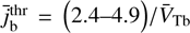 .
. -
The instability growth rate γmax (33) increases sharply with VTb once the threshold
 (20) is overcome (Fig. 7). This fast increase is caused by the fast demagnetization of the beam ions, in which case they cannot compensate for the perturbed currents of fully magnetized electrons. In a more distant overthreshold range
  the temperature dependence weakens because of the nearly saturated demagnetization.
 -
From the growth rate γmax (31) it follows that the instability can be strong, γmax ≳ 0.1ωBi, even for modest
 not far from the threshold. The most unstable wavenumber kzρTb ≳ 1.54 near the threshold
  , but increases with αb quickly approaching the asymptotic scaling kzρTb ~ b/2. In this asymptotic regime, our growth rate reduces to (35), the same as was obtained by Bell (2004).
 -
Two particular applications to the terrestrial foreshocks and supernova remnants show that the reactive CCPI can operate there. An analysis of Sect. 5.2 suggests that the ions reflected from the shocks around supernova remnants can drive stronger instability than the cosmic rays. In the terrestrial foreshock, CCPI can regulate beam parameters generating electromagnetic fluctuations observed at kzρTi ≈ 0.1.
Our results complement and extend previous studies on electromagnetic instabilities and their role in space and astrophysical plasmas. CCPI can develop around supernova remnants expanding into interstellar medium, participating in the braking process, and heating and redistributing energy in the supernova shocks. The same concerns the solar-wind regions upstream of the terrestrial bow shock, and other heliospheric shocks, where CCPI can bound the beam parameters and contribute to the low-frequency electromagnetic turbulence. Similarly, CCPI can affect other space and astrophysical environments containing super-Alfvénic ion beams and return currents.
Acknowledgments
This research was supported by the Belgian Science Policy Office (through Prodex/Cluster PEA 90316 and IAP Programme project P7/08 CHARM).
References
- Achterberg, A. 2013, MNRAS, 436, 705 [NASA ADS] [CrossRef] [Google Scholar]
- Alexandrov, A. F., Bogdankevič, L. S., & Rukhadze, A. A. 1984, Principles of Plasma Electrodynamics (Berlin: Springer-Verlag) [CrossRef] [Google Scholar]
- Amato, E., & Blasi, P. 2009, MNRAS, 392, 1591 [NASA ADS] [CrossRef] [Google Scholar]
- Artemyev, A. V., Rankin, R., & Vasko, I. Y. 2016, J. Geophys. Res., 121, 8361 [CrossRef] [Google Scholar]
- Bell, A. 2004, MNRAS, 353, 550 [Google Scholar]
- Bell, A. 2005, MNRAS, 358, 181 [NASA ADS] [CrossRef] [Google Scholar]
- Bret, A. 2009, ApJ, 699, 990 [NASA ADS] [CrossRef] [Google Scholar]
- Bret, A., Gremillet, L., & Dieckmann, M. E. 2010, Phys. Plasmas, 17, 120501 [NASA ADS] [CrossRef] [Google Scholar]
- Brown, M. R., Browning, P. K., Dieckmann, M. E., Furno, I., & Intrator, T. P. 2013, Space Sci. Rev., 178, 357 [NASA ADS] [CrossRef] [Google Scholar]
- Büchner, J., & Elkina, N. 2006, Phys. Plasmas, 13, 082304 [NASA ADS] [CrossRef] [Google Scholar]
- Chen, L., & Wu, D. J. 2012, ApJ, 754, 123 [NASA ADS] [CrossRef] [Google Scholar]
- Chen, C. H. K., Matteini, L., Schekochihin, A. A. et al. 2016, ApJ, 825, L26 [NASA ADS] [CrossRef] [Google Scholar]
- Duijveman, A., Hoyng, P., & Ionson, J. A. 1981, ApJ, 245, 721 [NASA ADS] [CrossRef] [Google Scholar]
- Gary, S. P. 1985, ApJ, 288, 342 [Google Scholar]
- Gary, S. P. 2005, Theory of Space Plasma Microinstabilities (Cambridge: Cambridge University Press) [Google Scholar]
- Gary, S. P., Foosland, D. W., Smith, C. W., Lee, M. A., & Goldstein, M. L. 1984, Phys. Fluids, 27, 1852 [NASA ADS] [CrossRef] [Google Scholar]
- Gary, S. P., Yin, L., Winske, D., & Reisenfeld, D. B. 2000, Geophys. Res. Lett., 27, 1355 [NASA ADS] [CrossRef] [Google Scholar]
- Hobara, Y., Walker, S. N., Balikhin, M. et al. 2007, J. Geophys. Res., 112, A07202 [NASA ADS] [CrossRef] [Google Scholar]
- Kobzar, O., Niemiec, J., Pohl, M., & Bohdan, A. 2017, MNRAS, 469, 4985 [NASA ADS] [CrossRef] [Google Scholar]
- Malovichko, P. P. 2007, Kinemat. Phys. Celest. Bodies, 23, 185 [NASA ADS] [CrossRef] [Google Scholar]
- Malovichko, P. P. 2010, Kinemat. Phys. Celest. Bodies, 26, 62 [NASA ADS] [CrossRef] [Google Scholar]
- Malovichko, P. P., & Iukhimuk, A. K. 1992, Kinematika i Fizika Nebesnykh Tel, 8, 20 [NASA ADS] [Google Scholar]
- Malovichko, P., Voitenko, Y., & De Keyser, J. 2014, ApJ, 780, 175 [NASA ADS] [CrossRef] [Google Scholar]
- Malovichko, P., Voitenko, Y., & De Keyser, J. 2015, MNRAS, 452, 4236 [NASA ADS] [CrossRef] [Google Scholar]
- Marcowith, A., Bret, A., Bykov, A. et al. 2016, Rep. Prog. Phys., 79, 046901 [NASA ADS] [CrossRef] [Google Scholar]
- Marsch, E. 2006, Liv. Rev. Sol. Phys., 3, 1 [Google Scholar]
- Marsch, E., & Livi, S. 1987, J. Geophys. Res., 92, 7263 [NASA ADS] [CrossRef] [Google Scholar]
- Mecheri, R. & Marsch, E. 2007, A&A, 474, 609 [NASA ADS] [CrossRef] [EDP Sciences] [Google Scholar]
- Narita, Y., Glassmeier, K.-H., & Fornaçon, K.-H. et al. 2006, J. Geophys. Res., 111, A01203 [NASA ADS] [CrossRef] [Google Scholar]
- Paschmann, G., Sckopke, N., & Papamastorakis, I. et al. 1981, J. Geophys. Res., 86, 4355 [NASA ADS] [CrossRef] [Google Scholar]
- Sentman, D., Edmiston, J. P., & Frank, L. A. 1981, J. Geophys. Res., 86, 2039 [Google Scholar]
- Schure, K. M., Bell, A. R., O’C Drury, L., & Bykov, A. M. 2012, Space Sci. Rev., 173, 491 [NASA ADS] [CrossRef] [EDP Sciences] [Google Scholar]
- Tsurutani, B., & Rodriguez, P. 1981, J. Geophys. Res., 86, A6, 4317 [NASA ADS] [CrossRef] [Google Scholar]
- Voitenko, Y. 1995, Sol. Phys., 161, 197 [NASA ADS] [CrossRef] [Google Scholar]
- Voitenko, Y. 1996, Sol. Phys., 168, 219 [NASA ADS] [CrossRef] [Google Scholar]
- Voitenko, Y. & Pierrard, V. 2015, Sol. Phys., 290, 1231 [NASA ADS] [CrossRef] [Google Scholar]
- Vojtenko Y. M., Krishtal’ A. N., Kuts S. V., Malovichko P. P., & Yukhimuk A. K. 1990, Geomagn. Aeron., 30, 901 [NASA ADS] [Google Scholar]
- Winske, D. & Leroy, M. M. 1984, J. Geophys. Res., 89, 2673 [NASA ADS] [CrossRef] [Google Scholar]
- Wu, D. J., Chen, L., & Wu, C. S. 2012, PhPl, 19, 024511 [NASA ADS] [CrossRef] [Google Scholar]
- Yoon, P. H., & Sarfraz, M. 2017, ApJ, 835, 246 [NASA ADS] [CrossRef] [Google Scholar]
- Zhao, J. S., Voitenko, Y., Yu, M. Y., Lu, J. Y., & Wu, D. J. 2014, ApJ, 793, 107 [NASA ADS] [CrossRef] [Google Scholar]
- Zweibel, E. G., & Everett, J. E. 2010, ApJ, 709, 1412 [NASA ADS] [CrossRef] [Google Scholar]
All Figures
|
Fig. 1. Instability threshold |
| In the text | |
|
Fig. 2. Illustration of the condition (18) for VA/Vb = 0.9 and αb = 6. In this case |
| In the text | |
|
Fig. 3. Illustration of the condition (18) for VA/Vb = 0:9 and αb = 10. In this case |
| In the text | |
|
Fig. 4. Unstable wavenumber ranges in the (αb, kz) plane for VA/Vb = 0.9. The outer boundary is defined by the left-hand side and the inner boundary by the right-hand side of condition (18). It is seen that below |
| In the text | |
|
Fig. 5. Wavenumber dependence of the instability growth rate driven by super-Alfvénic ion beams with VA/Vb = 0.9 for three values of αb: αb = 6, 8, and 10. For larger αb, the unstable area and the maximum growth rate extend to larger kzρTb. |
| In the text | |
|
Fig. 6. Normalized growth rate γmax/ωBi as a function of nb/n0 and Vb/VA for hot beam with VTb/VA = 102. γmax increases regularly with both nb/n0 and Vb/VA once the threshold is exceeded. |
| In the text | |
|
Fig. 7. Normalized growth rate γmax/ωBi as a function of VTb/VA for nbVb/ (n0VA) = 0.05 (solid curve), 0.1 (dotted curve), and 0.15 (dashed curve). Starting from zero, the growth rate γmax increases rapidly with VTb, but this increase is quickly saturated. Larger currents nbVb/ (n0VA) result in larger γmax for all VTb. |
| In the text | |
|
Fig. 8. Contribution of the reactive CCPI growth rate (dashed curve) to the total growth rate (dotted curve) for VTi/VA = Te/Ti = 1, Vb/VA = 10, VTb/VA = 25, and nb/n0 = 0.02. It is seen that the reactive destabilizing effects dominate the instability growth rate for this set of parameters. The wave frequency is shown by the solid line. |
| In the text | |
Current usage metrics show cumulative count of Article Views (full-text article views including HTML views, PDF and ePub downloads, according to the available data) and Abstracts Views on Vision4Press platform.
Data correspond to usage on the plateform after 2015. The current usage metrics is available 48-96 hours after online publication and is updated daily on week days.
Initial download of the metrics may take a while.