| Issue |
A&A
Volume 614, June 2018
|
|
|---|---|---|
| Article Number | A91 | |
| Number of page(s) | 28 | |
| Section | Stellar atmospheres | |
| DOI | https://doi.org/10.1051/0004-6361/201731678 | |
| Published online | 20 June 2018 | |
Wind properties of variable B supergiants
Evidence of pulsations connected with mass-loss episodes★
1
Departamento de Espectroscopía, Facultad de Ciencias Astronómicas y Geofísicas, Universidad Nacional de La Plata,
Paseo del Bosque s/n,
La Plata, Argentina
e-mail: This email address is being protected from spambots. You need JavaScript enabled to view it.
2
Instituto de Astrofísica de La Plata, CONICET-UNLP,
Paseo del Bosque s/n,
La Plata, Argentina
3
Instituto de Física y Astronomía, Facultad de Ciencias, Universidad de Valparaíso,
Av. Gran Bretaña 1111, Casilla 5030,
Valparaíso, Chile
4
Astronomický ústav, Akademie věd České republiky v.v.i.,
Fričova 298,
251 65
Ondřejov, Czech Republic
5
Tartu Observatory, Tõravere,
61602
Tartumaa, Estonia
Received:
31
July
2017
Accepted:
25
December
2017
Abstract
Context. Variable B supergiants (BSGs) constitute a heterogeneous group of stars with complex photometric and spectroscopic behaviours. They exhibit mass-loss variations and experience different types of oscillation modes, and there is growing evidence that variable stellar winds and photospheric pulsations are closely related.
Aims. To discuss the wind properties and variability of evolved B-type stars, we derive new stellar and wind parameters for a sample of 19 Galactic BSGs by fitting theoretical line profiles of H, He, and Si to the observed ones and compare them with previous determinations.
Methods. The synthetic line profiles are computed with the non-local thermodynamic equilibrium (NLTE) atmosphere code FASTWIND, with a β-law for hydrodynamics.
Results. The mass-loss rate of three stars has been obtained for the first time. The global properties of stellar winds of mid/late B supergiants are well represented by a β-law with β > 2. All stars follow the known empirical wind momentum–luminosity relationships, and the late BSGs show the trend of the mid BSGs. HD 75149 and HD 99953 display significant changes in the shape and intensity of the Hα line (from a pure absorption to a P Cygni profile, and vice versa). These stars have mass-loss variations of almost a factor of 2.8. A comparison among mass-loss rates from the literature reveals discrepancies of a factor of 1 to 7. This large variation is a consequence of the uncertainties in the determination of the stellar radius. Therefore, for a reliable comparison of these values we used the invariant parameter Qr. Based on this parameter, we find an empirical relationship that associates the amplitude of mass-loss variations with photometric/spectroscopic variability on timescales of tens of days. We find that stars located on the cool side of the bi-stability jump show a decrease in the ratio V∞∕Vesc, while their corresponding mass-loss rates are similar to or lower than the values found for stars on the hot side. Particularly, for those variable stars a decrease in V∞∕Vesc is accompanied by a decrease in Ṁ.
Conclusions. Our results also suggest that radial pulsation modes with periods longer than 6 days might be responsible for the wind variability in the mid/late-type. These radial modes might be identified with strange modes, which are known to facilitate (enhanced) mass loss. On the other hand, we propose that the wind behaviour of stars on the cool side of the bi-stability jump could fit with predictions of the δ−slow hydrodynamics solution for radiation-driven winds with highly variable ionization.
Key words: stars: early-type / supergiants / stars: mass-loss / stars: winds, outflows
Based on observations taken with the J. Sahade Telescope at Complejo Astronómico El Leoncito (CASLEO), operated under an agreement between the Consejo Nacional de Investigaciones Científicas y Técnicas de la República Argentina, the Secretaría de Ciencia y Tecnología de la Nación, and the National Universities of La Plata, Córdoba, and San Juan.
© ESO 2018
1 Introduction
Massive stars have a significant impact on the ionization, structure, and evolution of the interstellar medium (ISM). Via their stellar winds they release energy and momentum to their surroundings leading to the formation of stellar wind-blown bubbles, bow-shocks, and circumstellar shells. On the other hand, the huge amount of mass lost from the stars modifies the later stages of their lives (evolutionary timescales and final core masses) as well as the type of SN remnants left (Meynet et al. 1994; Woosley et al. 2002). Stellar winds of hot massive stars are mainly driven by line scattering of UV photons coming from the stars’ continuum radiation. The standard stationary radiation-driven wind theory (Castor et al. 1975; Pauldrach et al. 1986; Friend & Abbott 1986) predicts mass-loss rates and terminal velocities as a function of stellar parameters (Abbott 1982; Vink 2000; Vink et al. 2001), and also predicts a wind momentum–luminosity relationship (WLR; Kudritzki et al. 1995). This theory has long described the global properties of stellar winds of OBA stars. However, advances in the observational techniques (high spatial and spectral resolution) together with progress in more realistic atmosphere models have revealed discrepancies in the mass-loss rates not only between theory and observations, but also amongst different observational tracers themselves (cf. Puls et al. 2008).
As Owocki & Rybicki (1984), Owocki et al. (1988), and later Feldmeier (1998) demonstrated, strong hydrodynamic instabilities occur in line-driven winds of massive O-type stars, leading to the formation of wind-clumping (small-scale density inhomogeneities distributed across the wind). Wind-clumping has traditionally been used to solve the issue of the mass-loss discrepancy found in O supergiants (OSGs) when different diagnostic methods are employed (Bouret et al. 2005; Fullerton et al. 2006). Mass-loss rates derived from unsaturated UV resonance lines give lower values than those obtained from the Hα line (cf. Puls et al. 2008). The macroclumping approach (with optically thick clumps at certain frequencies) has provided a fully self-consistent and simultaneous fit to both UV and optical lines (Oskinova et al. 2007; Sundqvist et al. 2010, 2011; Šurlan et al. 2013). In previous works an artificial reduction of the stellar mass-loss rate, an extremely high clumping factor, or an anomalous chemical abundance for specific elements were invoked; however, the macroclumping approach means that none of these is necessary.
The situation is different for B supergiants (BSGs). Stellar winds of BSGs are fairly well represented by the analytical velocity β-law, with β typically in the range 1−3 (Crowther et al. 2006; Markova & Puls 2008). Moreover, these stars show a drop in the ratio V∞ ∕Vesc of a factor of two at around 21 000 K, from 2.6 for stars on the hot side to 1.3 for stars on the cool side (Pauldrach & Puls 1990), known as the bi-stability jump (Lamers et al. 1995). This jump was interpreted as a consequence of the recombination of Fe IV to Fe III in the wind (Vink et al. 1999). These authors predicted that this drop should be accompanied by a steep increase in the mass-loss rate of about a factor of 3 to 5, whilst some observations indicate a decrease (Crowther et al. 2006; Markova & Puls 2008). A recent study of the effects of micro- and macroclumping in the opacity behaviour of the Hα line at the bi-stability jump suggests that the macroclumping should also play an important role at temperatures on the cool side of the jump (Petrov et al. 2014).
It is also well known that stellar winds of BSGs are highly variable. To date, most of the studies related to α Cyg variables and hypergiants have focused on their photometric and/or optical spectroscopic (mainly Hα) variability, and many surveys have been carried out to search for variability periods (e.g. Kaufer et al. 2006; Lefever et al. 2007; Lefèvre et al. 2009). Long-term space-based photometry and spectroscopy have linked this variability to opacity-driven radial and non-radial oscillations (Glatzel et al. 1999; Lefever et al. 2007; Kraus et al. 2015), and new instability domains have been established in the Hertzsprung–Russell (HR) diagram covering the region of BSGs (Saio et al. 2006; Godart et al. 2017). As massive stars can cross the BSGs’ domain more than once, the pulsation activity of these stars can drastically change between their red- and blue-ward evolution (Saio et al. 2013). BSGs on a blue-ward evolution (i.e. a post-red supergiant) tend to undergo a significantly larger number of pulsations, even including radial strange-mode pulsations with periods between 10 and 100 days (or more). It has been suggested that strange-mode pulsations cause time-variable mass-loss rates in very luminous evolved massive stars (Glatzel et al. 1999). The first observational evidence of the presence of strange modes have been found in two BSGs: HD 50064 (Aerts et al. 2010) and 55 Cyg (Kraus et al. 2015). In the latter, the authors found line variations with periods in the range of 2.7 h to 22.5 days. They interpreted these variations in terms of oscillations in p-, g-, and strange modes. The last could lead to phases of enhanced mass loss. Finally, the connection between pulsation and mass loss in 55 Cyg was confirmed by Yadav & Glatzel (2016), based on a linear non-adiabatic stability analysis with respect to radial perturbations. These authors demonstrated that, as a consequence of the instabilities, the non-linear simulations revealed finite amplitude pulsations consistent with the observations.
To obtain further insights on the wind structure and wind variability of evolved stars of intermediate mass, we studied a sample of Galactic BSGs (classified either as irregular or α Cyg-type variables) in both the blue and the Hα spectral region. The Hα emission is quite sensitive to the wind properties (Puls et al. 2008), and we used the Fast Analysis of STellar atmospheres with WINDs (FASTWIND; Santolaya-Rey et al. 1997; Puls et al. 2005; Rivero González et al. 2012) to obtain terminal velocities and mass-loss rates by fitting synthetic to observed line profiles. In addition, to derive proper stellar parameters (effective temperature and surface gravity) we consistently modelled the Si ionization balance together with the photospheric lines of H and He. Determining new, more accurate values of mass-loss rates and stellar parameters of massive stars is crucial for our understanding of stellar wind properties, wind interactions with its surroundings, and the plausible mechanisms related with wind variability and its evolution.
The paper is structured as follows: our observations and modelling are described in Sects. 2 and 3, respectively. The results of our line profile fittings are shown in Sect. 4 and the new wind parameters are compared with previous determinations. For three objects (HD 74371, HD 99953, and HD 111973) the wind parameters are reported for the first time. As most of the stars in our sample exhibit photometric and spectroscopic variability, on timescales from one to tens of days, and have been modelled previously by several authors, in Sect. 5 we discuss changes in the wind parameters. We present for mid and late BSGs an empirical relationship between the amplitude of mass-loss variations and light/spectroscopic periods, indicating that a significant percentage of the mass-loss could be triggered by pulsation modes. Our conclusions are given in Sect. 6. Finally, Appendix A shows model fittings to the photospheric lines of each star and summarizes the stellar and wind parameters found in the literature and in this work.
2 Observations
We took high-quality optical spectra for 19 Galactic BSGs of spectral types between B0 and B9. These stars were selected from the Bright Star Catalog (Hoffleit & Jaschek 1991). The observations were performed in January 2006, February 2013, April 2014, and February and March 2015. We used the REOSC spectrograph (in crossed dispersion mode) attached to the Jorge Sahade 2.15 m telescope at the Complejo Astronómico El Leoncito (CASLEO), San Juan, Argentina. The adopted instrumental configuration was a 400 l/mm grating (#580), a single slit of width 250 μ, and a 1024×1024 TEK CCD detector with a gain of 1.98 e−/ adu. This configuration produces spectral resolutions of R ~ 12 600 at 4500 Å and R ~ 13 900 at 6500 Å. Spectra were reduced and wavelength calibrated following the standard procedures using the corresponding IRAF1 routines. The resulting spectra have an average signal-to-noise ratio (S/N) of ~300.
Table 1 lists the stars in our programme, indicating name and HD number, spectral type, and variable type designation according to (Lefèvre et al. 2009); from a study of HIPPARCOS light curves or the VSX database. In addition, binary stars are also listed. In the following columns of the same table, we list the reported light curve or spectroscopic periods, the observation dates of our data, and the achieved wavelength coverage. Here, we present six stars with more than one observation (HD 53138, HD 58350, HD 75149, HD 80077, HD 99953, and HD 111973). One of these stars (HD 111973) was observed on two consecutive nights.
Log of observations
3 Stellar and wind parameters
To derive stellar and wind parameters we made use of the code FASTWIND (v10.1.7). The code computes a spherically expanding line-blanketed atmosphere. All background elements are considered with their solar abundances (taken from Grevesse & Sauval 1998). H, He, and Si atoms are treated explicitly with high precision by means of a complete NLTE approach and an accelerated lambda iteration (ALI) scheme is applied to solve the comoving-frame equations of radiative transfer (Puls 1991). The atmospheric stratification is modelled considering a smooth transition between a quasi-hydrostatic photosphere and an analytical wind structure described by a velocity β-law. The temperature structure is calculated from the electron thermal balance and is consistent with the radiative equilibrium condition.
We opted for a wind model without clumping because we want to compare the derived mass-loss rates with previous determinations and to study the wind variability. In general, mass-loss rates found in the literature are mainly estimated using unclumped models. A second reason is that we do not have contemporaneous data in the UV and IR spectral regions to evaluate the importance of the clumping factor in the Hα line modelling. As a consequence, our results will provide upper-limit values for the mass-loss rates. In addition, to obtain an optimal fit to the observed line profiles, it was necessary to consider not only a microturbulence velocity, Vmicro, and broadening due to the star’s rotation, V sin i, but also the effect of a macroturbulence velocity, Vmacro. The latter contributes mainly to line broadening and shaping as noted by Simón-Díaz & Herrero (2007).
To obtain the effective temperature (Teff) we evaluated the ionization balance (e.g. Si II−Si III, Si III−Si IV, if the Si IV λ 4089, 4116 lines are observed, and He I−He II). We used solar abundances for He and Si (log NHe∕NH = −1.07 and log NSi∕NH = −4.45) and found good fits for each modelled spectrum (see details in Sects. 4.1 and 5). To derive an accurate determination of the surface gravity (log g), we modelled the Hγ and Hδ lines. We used a “by eye” fitting procedure to find the best-fitting synthetic line spectrum to the observed one.
The Hα line was modelled to derive the mass-loss rate (Ṁ) and the parameters of the velocity β-law: the power index β and the terminal velocity V∞. It is important to stress that the major source of uncertainty in the determination of mass-loss rates is due to ambiguous determinations of stellar radii and distances to the stars (see Markova et al. 2004). On the other hand, Hα is rather sensitive to V∞ (Garcia et al. 2017). Therefore, the stellar radius and terminal velocities should be derived independently, as explained below.
Prior to the modelling process, the stellar radius, R⋆, was derived using the measured angular diameter, the distance to the star, or a fit to the observed spectral energy distribution (SED). We model the SED with the interactive user interface BeSOS2 using the best-fitting atmospheric (TLUSTY or Kurucz) model (Hubeny & Lanz 1995; Kurucz 1979). BeSOS reads stellar photometry data of any star from photometry-enabled catalogues in VizieR and the parallax distance from the HIPPARCOS catalogue. Sometimes, it was not possible to obtain a good fit to the SED (see details below on the procedures applied to each star). In these cases, a slightly modified distance was required to improve the fit. To find the best model, BeSOS uses the IDL program mpfit that searches for the best fit using the Levenberg–Marquardt (LM) method, which is a standard technique for solving non-linear least squares problems.
BeSOS provides, for a given colour excess, a new set of stellar parameters: Teff, log g, and R⋆ (in units of the solar radius). As initial entries we use the Teff and log g values obtained in this work from the Si and He ionization balances and from Hγ and Hδ line widths, respectively, and the code searches then for the most optimal values to fit the SED. The colour excess, E(B − V), was calculated using the observed B − V and the interpolated  values calculated from the Teff − (B − V) scale for supergiants (Flower 1996). In a few cases, the E(B − V) had to be modified to fit the 2200 Å bump properly. The stellar radius obtained using the SED is averaged with the values derived via the angular diameter and Mbol (the bolometric magnitude). Table 2 lists the intrinsic properties for each star: the spectral type found in the literature, the visual apparent magnitude, the observed and intrinsic colour indexes, the calculated colour excess, the stellar parameters (Teff and log g, obtained from fittings to the SED), the distance to the star (d), the bolometric correction (BC), the calculated bolometric magnitude, and the stellar radius. The computed parameters are listed with their corresponding errors. Details on the best-fitting model obtained with BeSOS are given in Sect. 4.
Typical error bars derived using the BESOS code for Teff, log g, and R⋆ are of about 1%, 2%, and 5%, respectively.Nevertheless, considering uncertainties in the distance estimates between 5% and 30% (from parallax measurements) and differences less than 1500 K between the Teff values derived from BESOS and FASTWIND, the propagation of errors yields an uncertainty in Mbol lower than 10% and a margin of error between 5% and 20% for R⋆.
In relation to the stellar parameters derived from FASTWIND, we can adopt the parameter errors estimated by Kraus et al. (2015), who found uncertainties in Teff of 300–500 K from the Si ionization balance and 1000 K for the He lines. We adopt Δ Teff= 1000 K for those stars for which only the He lines were modelled and ΔTeff = 500 K if the Si II, Si III, and He lines were used to derive the temperature. From measurements of the wings of Hγ and Hδ we estimated an error of 0.1 dex in log g. The error bars in Vmicro are 2 km s−1 for Si and He lines, 5 km s−1 for the H lines, and 10 km s−1 for Hα. We model all the photospheric lines using the same Vmicro.
Both V sin i and Vmacro affect the line broadening. To model the line profiles we adopted the value of V sin i (± 10 km s−1) found in the literature (Kudritzki et al. 1999; Lefever et al. 2007; Fraser et al. 2010, given in Table A.1) or average values when large scatters are present. We derived the macroturbulent velocity that reproduces the extra broadening seen in the line profile. We found uncertainties in Vmacro from 10 km s−1 to 20 km s−1.
Regarding the wind parameters, we searched for V∞ measurements from UV observations (Prinja & Massa 2010; Prinja et al. 1998; Howarth et al. 1997) and used them as initial values to reproduce the Hα line. Good fits were obtained using slight variations of V∞. These values are listed in Table 3 with deviations of 10% with respect to the UV measurements. In a few cases, the UV terminal velocities were not able to fit the observed Hα line profile and our ownV∞ determinations are provided. In this case, the discrepancies obtained between the derived V∞ and the UV data can increase up to 30%. Therefore, we consider errors for V∞ between 10% and 30%.
Adopting the values for V∞ from the UVand errors of 10% for R⋆, we observe that late and early B supergiants may show a change of up to 20% in the equivalent width (EW) of the emission component of a P Cygni line profile if Ṁ varies by an amount of 10% and 20%, respectively. Larger errors in V∞ might give uncertainties on Ṁ of 30%. However, when the Hα line is seen in absorption, the error on Ṁ can be larger than a factor of 2 (Markova et al. 2004).
4 Results
For each star in our programme we modelled the line profiles of H, He, and Si. Figure 1 shows the observed Hα line and the best-fitting synthetic model. The rest of the lines and their corresponding fits are shown in the Appendix (Figs. A.1–A.7). In Table 3 we list the obtained stellar and wind parameters with their errors: Teff, log g, β, Ṁ, V∞, Vmicro, Vmacro, V sin i, R⋆ (stellar radius in solar radius units), logL∕L⊙ (stellar luminosity referenced to the solar value), log Dmom (the modified wind momentum rate, see Sect. 5), log L∕M (both L and M in solar units, where M is the stellar mass), and Q (optical-depth invariant, discussed in Sect. 5). The parameters Vmicro and Vmacro are related to the photospheric lines. Initially Vmicro was fixed at 10 km s−1 and then varied by ± 5 km s−1 to achieve the best fit to the intensities of He and Si lines.
The photospheric lines of each star (at a given epoch) were modelled with the same set of Vmicro and Vmacro values. However, to properly match the Hα and He I λ 6678 line widths and shapes we often needed a different turbulent velocity since these lines are affected by the velocity dispersion of the flow.
Regarding the determination of the wind parameters, we were able to reproduce the Hα line of many BSGs. However, in a few cases, even when the emission component of the P Cygni profile looked well fitted, it was impossible to reproduce the intensity of the absorption component. Similar problems were found when reproducing the Hα absorption profile of HD 38771, HD 75149, and HD 111973 because of the presence of an incipient emission in the line core. Contrary to the Hα line, synthetic line profiles of the photospheric lines match the observations very well.
Stellar parameters calculated in the present study or adopted from the literature.
4.1 Comments on individual objects
In the following we summarize the previous and current data of the stellar and wind parameters for each star. In addition, we complement our data with images taken with the Wide-field Infrared Survey Explorer (WISE; Wright et al. 2010), covering the range 3.5 μ–22 μ (bands W1 and W4). These images are used to identify former phases of strong stellar winds.
HD 34085 is a B8 Iae star that has been studied by many authors. Using FASTWIND we estimated the stellar fundamental parameters: Teff = 12 700 K and log g = 1.7. The best-fitting model to the SED was obtained with the BeSOS interactive interface using a Kurucz model with Teff = 11 760 K, log g = 2.0, R⋆ = 71 R⊙, E(B − V) = 0.044 (calculated as explained in Sect. 3), and d = 259 pc (which is close to the distance of 264 pc given by HIPPARCOS). Using the HIPPARCOS distance and the mentioned value of E(B − V), we estimated Mbol = − 7.95 mag and R⋆ = 70 R⊙; instead, from the angular diameter (2.713 mas, Zorec et al. 2009) we calculated R⋆ = 76 R⊙. We assumed a mean value for this star of R⋆ = 72 R⊙.
Our estimate of Teff (12 700 K) agrees with previous determinations (see Table A.1). This star shows a photometricvariation of 2.075 days (Lefèvre et al. 2009). Moreover, Moravveji et al. (2012) found 19 significant pulsation modes from radial velocities with variability timescales ranging from 1.22 days to 74.74 days. It also presents a variable stellar wind with changes in the mass-loss rate of at least 20% on a timescale of one year (Chesneau et al. 2014). Using spectro-interferometric monitoring, these authors found time variations in the differential visibilities and phases. For some epochs, the temporal evolution of the signal suggests the rotation of circumstellar structures. However, at some periods, no phase signal was observed at all. This result was interpreted in the context of second-order perturbations of an underlying spherical wind.
The Hα line is highly variable (with profiles in absorption, filled in by emission, double-peaked, or inversed P Cygni; Chesneau et al. 2014). Our observation resembles the one reported by Przybilla et al. (2006). Our estimate for the mass-loss rate is ~ 1.5 times lower than the value obtained by Markova et al. (2008), and at least one-third of the value reported by Chesneau et al. (2014). We also derive a low terminal velocity. This value is quite uncertain because we were not able to fit the absorption component of the Hα P Cygni profile. Moreover, a high Vmacro (85 km s−1) was needed to reproduce the emission component of the line profile. The photospheric lines were modelled very well, with the exception of the He I λ 4471 line, which does not exhibit the forbidden component.
HD 38771 (B0.5Ia): the stellar and wind parameters of this star have been derived by many authors: Nerney (1980), Garmany et al. (1981), Lamers et al. (1982), Kudritzki et al. (1999), Crowther et al. (2006), Searle et al. (2008), Zorec et al. (2009). Their values range from 26 000 K to 27 500 K in Teff, from 2.9 dex to 3.07 dex in log g, from 13.0 R⊙ to 28 R⊙ in stellar radius, from 0.27 × 10⁻⁶ M⊙ yr−1 to 1.20 × 10⁻⁶ M⊙ yr−1 in  , and from 1350 km s−1 to 1870 km s−1 in V∞ (see Table A.1). The star presents a variable magnetic field (Nerney 1980) and exhibits spectral variations. The observed Hα line is quite variable, showing a pure absorption profile (Kudritzki et al. 1999), a double-peaked absorption profile with a central emission (Rusconi et al. 1980), and an absorption profile with a strong central emission (Crowther et al. 2006). Morel et al. (2004) also described changes in morphology and profile amplitude of 32.6%, which clearly suggest variations in the wind conditions. These authors also found two photometric periods of 4.76 and 1.047 days and Prinja et al. (2004) reported additional spectroscopic periods of 1.9, 6.5, and 9.5 days.
At the time of our observation the Hα line displayed an asymmetric absorption profile with a weak emission in the core (Fig. 1). We also note that the core of the Hβ line might be filled in by an incipient emission (Fig. A.1). Extra broadening effects are present in all the photospheric lines leading to large Vmacro estimates (of the order of the projected rotation velocity).
We derived Teff = 25 000 K using Si II and Si III, and also using the He I and He II ionization balance. The best-fitting SED model was obtained with a TLUSTY model for Teff = 25 700 K, log g = 2.70, R⋆ = 14 R⊙, and E(B − V) = 0.05 mag for a distance of 191 pc (close to the HIPPARCOS distance of dH= 198 pc; van Leeuwen 2007). Using dH in Pogson’s formula we derived a Mbol = –6.99 mag and R⋆ ~ 12 R⊙. The adopted stellar radius, R⋆ ~ 13 R⊙, which is consistent with the value derived from the angular diameter calculated by Zorec et al. (2009, 0.62 mas).
Our Teff value is 1000 K lower than the values obtained by Searle et al. (2008) and Gathier et al. (1981), while the stellar radius is similar to that obtained by Kudritzki et al. (1999). Compared with previous determinations, our mass-loss rate has the lowest value. As Hα is in pure absorption Ṁ might have a large uncertainty.
Considering the diversity of the stellar and wind parameters found in the literature, and that the Hα line profile shows important variations, this star is a good candidate to search for pulsating or magnetic activity connected to cyclic wind variability.
HD 41117 (B2Ia): this is another deeply studied star (Zorec et al. 2009; Crowther et al. 2006; Morel et al. 2004; Kudritzki et al. 1999; Scuderi et al. 1998; Nerney 1980). Morel et al. (2004) found Hα variations, both in shape and intensity, and reported light variability on a period of 2.869 days. Additional sets of spectroscopic periods were obtained from Hα equivalent width time series (Morel et al. 2004, Table 1).
From Table A.1 we see that the fundamental stellar parameters and luminosity are consistent with those already published, in contrast with the wind parameters (mainly Ṁ) that are quite different (by a factor of up to 3.6).
The best-fitting SED model corresponds to Teff = 17 940 K, log g = 2.2, R⋆ = 26 R⊙, E(B − V) = 0.42 mag (instead we derived E(B − V) = 0.46 mag from Flower 1996) and d = 477 pc (while the distance measured by HIPPARCOS is 552 ± 85 pc). On the other hand, using d = 447 pc and E(B − V), the angular diameter (0.371 mas, Zorec et al. 2009), or the computed bolometric magnitude (− 7.35 mag) the stellar radius is R⋆ ~ 23 R⊙. We therefore adopted R⋆ = 23 R⊙, which is also consistent with the stellar radius expected from the HIPPARCOS distance. The stellar radius is lower than the value derived by other authors (see Table A.1); however, if we use the distance derived by Megier et al. (2009, 1.62 kpc) we obtain R⋆ = 62 R⊙.
From the line modelling we obtained higher Teff = 19 500 K and log g = 2.3 values. Our spectrum reveals a Hα emission line with a complex blue-ward absorption component (see Fig. 1). The mass-loss rate derived here is lower (by a factor of about 5) than the value reported by Kudritzki et al. (1999). We also obtained a lower terminal velocity. The rest of the lines are in pure absorption and are excellently modelled (see Fig. A.1). Values of Vmicro and Vmacro as high as the rotational velocity of the star (V sin i = 40 km s−1) are needed to reproduce the extra broadening of the photospheric lines. A larger macroturbulent velocity (65 km s−1) was also obtained by Simón-Díaz & Herrero (2014).
HD 42087 (B4Ia): the SED was fitted with a TLUSTY model using Teff = 15 000 K, log g = 2.39, R⋆ = 60 R⊙, E(B − V) = 0.34 mag, and d = 2 021 pc (which is similar to the distance of 2 075 pc derived by Megier et al. 2009, from the Ca II H+K lines). On the other hand, a distance d = 2 075 pc gives Mbol = −8.33 mag and R⋆ = 50 R⊙, while the angular distance calculated by Zorec et al. (2009) leads to R⋆ = 57 R⊙. We adopted a mean value of R⋆ = 55 R⊙.
Our optical spectrum only covers the Hα region; therefore, we were not able to determine the effective temperature using the silicon lines. Thus, we adopted the value calculated by Zorec et al. (2009) (Teff = 16 500 K) and derived from the H lines a log g = 2.45. This Teff is lower than the value reported by Benaglia et al. (2007) and Searle et al. (2008), and greater than the value we derived from the fitting of the SED.
This star presents a significant Hα variability of 91.2% and both the Hα and He I λ6678 lines show a cyclic behaviour on a periodicity of ~25 days (Morel et al. 2004). This period is larger than the 6.807 day period found from the HIPPARCOS light curve (Morel et al. 2004; Lefèvre et al. 2009).
Our Hα line shows a P Cygni feature with a weak emission and a broad absorption component with a superimposed incipient emission structure. We fitted the Hα line profile using a wind model with Ṁ = 0.57 10−6 M⊙ yr−1 and V∞ = 700 km s−1. The obtained V∞ is similar to the one measured in the UV spectral range (735 km s−1, Howarth et al. 1997).
HD 47240 is a fast rotating B1Ib star (V sin i = 114 km s−1, Simón-Díaz & Herrero 2014) that lies behind the Monoceros Loop supernova remnant (SNR). It presents very broad photospheric absorption lines, periodic light variations of 2.742 days (Lefèvre et al. 2009; Morel et al. 2004), periodic motions due to binarity, and the presence of discrete absorption components (DACs; Prinja et al. 2002) that appear double. We were able to get a good fit to the SED for the following parameters: Teff = 17 500 K, log g = 2.4, E(B − V) = 0.33 mag, d = 1515 pc, and R⋆ = 35 R⊙. The derived distance is consistent with the distance estimate of 1598 pc by Megier et al. (2009) and the colour excess also matches the 2200 Å bump. We also calculated a Mbol = − 7.66 mag and R⋆ = 28 R⊙ (for d = 1598 pc). This stellar radius agrees with the computed value from the angular diameter (0.157 mas) by Zorec et al. (2009). We adopted a mean value of R⋆ = 30 R⊙.
The stellar parameters derived with FASTWIND agree with the values given in one of the models calculated by (Lefever et al. 2007); who found two models with very different Teff and log g and both fit very well the Si III line profiles. The Teff obtained here is lower than the 21 670 K derived with the BCD spectrophotometric method (Zorec et al. 2009).
To model the photospheric lines we needed a high Vmacro value (60 km s−1) that is much higher than those used to model the H lines formed in the wind (3 km s−1). As this object is a pulsating variable star of α Cyg type, a high Vmacro value is expected.
Our spectrum shows Hα as a double-peaked emission line with an intense central absorption. This profile was considered as an indicator of the presence of a disk-like structure (Lefever et al. 2007). We achieved a good fit to the observed Hα line for the intensity of the absorption and for the two emission components. We derived a mass-loss rate of 2.4 × 10⁻⁷M⊙ yr−1. This value agrees with the upper limit of the range reported by Lefever et al. (2007, 1.7 × 10⁻⁷ M⊙ yr−1 – 2.4 × 10⁻⁷ M⊙ yr−1) and is lower than the value calculated by Morel et al. (2004, 0.31 × 10⁻⁷ M⊙ yr-1) from the theoretical WLR for OBA supergiants. For the terminal velocity, we found almost half of the value obtained by Lefever et al. (2007), Prinja & Massa (2013).
HD 52089 (B1.5 II) is the brightest EUV source in the sky. It shows a UV emission line spectrum and X-ray emission consistent with a wind-shock model. Using the observed SED and TLUSTY models we derived Teff= 21 000 K, log g = 3.0, and R⋆ = 11 R⊙ for a distance of 124 pc (van Leeuwen 2007) and E(B − V) = 0.00 mag. This stellar radius is also consistent with the bolometric magnitude (Mbol= –6.18 mag) and the measurement of the angular diameter (0.801 mas, Zorec et al. 2009) that lead to 10 R⊙ and 10.6 R⊙, respectively. From FASTWIND we derived a higher Teff (23 000 K) that agrees with the values given in Lefever et al. (2010), Zorec et al. (2009), and Morel et al. (2008), but it is higher than the value of 20 100 K obtained by Fraser et al. (2010). Our surface gravity value (3 dex) agrees more closely with the Fraser et al. (2010) estimate and it is 0.2 dex lower than those reported by Lefever et al. (2010) and Morel et al. (2008). The star has a longitudinal magnetic field of 149 G (Morel et al. 2008). Our spectrum displays all the H lines in absorption. Using optical data we derive a mass-loss rate of 2 × 10⁻⁸ M⊙ yr−1, which is similar to the value obtained phenomenologically by Cohen et al. (1996, 3 × 10⁻⁸ M⊙ yr−1–8 × 10⁻⁸ M⊙ yr−1).
HD 52382 (B1Ia) is an O-B2 runaway candidate (Peri et al. 2012). Using FASTWIND to fit the ratios of Si III/Si II and He II/He I we obtain Teff = 21 500 K, and from the Hγ and Hδ lines a log g = 2.45. From Flower (1996) we have  = –0.20 mag and derive a colour excess of 0.39 mag. The best fit to the observed SED corresponds to a TLUSTY model with Teff = 23 140 K, log g = 2.47, R⋆ = 21.6 R⊙, and d = 1.23 kpc, but with a larger E(B − V) = 0.44 mag. This distance agrees with the 1.1 kpc found by Megier et al. (2009) and with the parallactic distance of 1.3 kpc measured by Gaia (0.768 mas; Astraatmadja & Bailer-Jones 2016). Using the distance of 1.3 kpc in Pogson’s formula and the expression for the angular radius (with 0.17 mas; Pasinetti Fracassini et al. 2001), we obtain a stellar radius of 18.6 R⊙ and 23.5 R⊙, respectively. Therefore, we adopted R⊙ = 21 R⊙ as the mean value. We rejected the HIPPARCOS distance of 471 pc because it leads to a value of Mbol that is too low for a B supergiant.
The derived Teff = 21 500 K is between the values calculated by Lefever et al. (2010) and Krtička & Kubát (2001). The star presents a variable Hα line profile displaying a P Cygni or a pure emission feature (Morel et al. 2004). Our spectrum shows a pure emission line. We were able to reproduce all the spectral lines very well. We derived a terminal velocity of 1000 km s−1, which is of the same order as that obtained from the UV region (900 km s−1, Prinja et al. 1990), but 200 km s−1 lower than the value found by Krtička & Kubát (2001) for a similar mass-loss rate. The combined WISE W2, W3, and W4 images (Fig. 2, at 4.6 μm, 12 μm, and 22 μm, respectively) reveal a complex structure close to the star and in the direction of its proper motion (indicated in Fig. 2 with a white arrow) that could be related to wind interactions with the ISM, due to high mass-loss episodes in the past.
We want to stress that for an optimal fitting of the photospheric lines we have to introduce high values of Vmacro, of around 65 km s−1 (a similar result was reported by Lefever et al. 2010), which could be an indication of pulsation activity. The He I λ 6678 line shows a little emission in the core.
HD 53138 (B3Ia) has been studied by several authors (see summary in Table A.1). The derived Teff ranges from 15 400 K to 18 500 K, and log g from 2.05 dex to 2.35 dex. The star exhibits irregular variations in the Hα line (Morel et al. 2004). Our spectra also show variations: in 2006 the star displayed a typical P Cygni profile, while in 2013 a double-peaked emission was observed. We also note differences in the intensities and line widths of the Hγ and the Si III lines for the two epochs that lead to slightly different values of Teff and log g. We obtained for both epochs the following fundamental parameters: 18 000 K for Teff and 2.25 dex for log g with uncertainties of 1000 K and 0.2 dex. The best-fitting SED model suggests Teff = 18 000 K, log g = 2.2, R⋆ = 46 R⊙, d = 822 pc (close to 847 pc the HIPPARCOS estimate), and E(B − V) = 0.10 (lower than the colour excess of 0.131 mag we obtained from Flower 1996). The calculation of R⋆ by means of the angular diameter gives 51 R⊙, while the computed Mbol (–8.53 mag) suggests R⋆ = 46 R⊙. We adopted R⋆= 46 R⊙.
The photospheric lines are broadened by macroturbulent motion (Vmacro = 60 km s−1). This high value of Vmacro, which is almost twice the measured value for the projected rotation velocity, is consistent with the suggestion of a pulsating variable star of α Cyg type (Lefèvre et al. 2009).
Our model fits the observed He Iλ 4471 Å line and the emission component of Hα fairly well, although we were not able to reproduce the absorption component of the profile in 2006 or the emission component observed in 2013. Our mass-loss estimates are in the range of previously determined values of other authors, being higher in 2006. The terminal velocity measured in the spectrum of 2013 is lower than in 2006 (see Table A.1). Barlow & Cohen (1977) measured a significant infrared excess at 10 μm requiring a mass-loss rate a factor of 20 times higher than ours to account for it.
HD 58350 (B5Ia) is an MK standard star. The set of stellar parameters derived with FASTWIND (log g and Teff) agrees very well with those derived by McErlean et al. (1999), Searle et al. (2008), Fraser et al. (2010). We were not been able to obtain a good fit to the SED using simultaneously the UV, visual, and IR photometry. However, based on the distance given by HIPPARCOS (609 pc) and the calculated angular diameter (0.882 mas, Zorec et al. 2009), we obtained R⋆ = 57 R⊙. Based on HIPPARCOS parallax measurement and the derived E(B − V) = 0.083 mag from Flower (1996), we obtained Mbol = −7.97 mag and R⋆ = 51 R⊙. We adopted R⋆ = 54 R⊙ as the mean value.
The Hα line shows a variable P Cygni profile with a tiny emission component. We were able to match the observations taken in 2006 and to get a fairly good fit to the one acquired in 2013. In the former, we failed to fit the absorption component. Our mass-loss rate is similar to that given by Lefever et al. (2007) and lower than the value given by Searle et al. (2008). As these last authors do not show the stellar spectrum in the Hα region, we cannot discuss the origin of the discrepancies. Morel et al. (2004) show time-series of the Hα line where the profile is seen in absorption, while the observations of Ebbets (1982) display a P Cygni profile. The light curve presents one period of 4.70 days (Koen & Eyer 2002) and another one of 6.631 days (Lefever et al. 2007).
HD 64760 (B0.5Ib) is a rapid rotator. The star was extensively studied as part of the IUE “MEGA Campaign” by Massa et al. (1995) and Prinja et al. (1995). The line variability observed in the UV argues in favour of rotationally modulated wind variations. It displays a double-peaked emission line profile in Hα and very broad absorption lines of H and He. Direct observations reveal a connection between multi-periodic non-radial pulsations (NRPs) in the photosphere and spatially structured winds (Kaufer et al. 2006). These observations also seem to be compatible with the presence of co-rotating interaction regions.
The fitting of the SED provides the following parameters: Teff = 22 370 K, log g = 2.50, R⋆ = 15 R⊙, E(B − V) = 0.07 mag, and d = 486 pc (while HIPPARCOS parallax gives d = 507 pc). The derived Mbol = –6.72 mag gives R⋆ = 12 R⊙, while the angular diameter leads to R⋆ = 10 R⊙. We adopted R⋆ = 12 R⊙ as the mean value.
Our stellar parameters derived with FASTWIND (Teff = 23 000 K, log g = 2.90) agree fairly well with those of Lefever et al. (2007), but show large discrepancies with the values reported by Searle et al. (2008). Although Searle et al. (2008) do not show the spectrum, they mentioned some difficulties in deriving accurate values from the models due to the large width of the spectral lines.
In general, we obtained very good fits for all the lines, even for the double-peaked Hα profile. Our model gives the same set of wind parameters as Lefever et al. (2007), but for the stellar radius a half of the value published by these authors was obtained. The combined WISE W1 and W4 images (3.4 μm and 22 μm, respectively) show the presence of either a double visual component or a wind-lobe structure (see Fig. 3).
HD 74371 (B6Iab/b) displays light variations with periods of 5− 20 days (van Genderen et al. 1989) and 8.291 days (Koen & Eyer 2002; Lefèvre et al. 2009). The stellar parameters Teff and log g were determined by Fraser et al. (2010) and agree very well with the values that we derived with FASTWIND (Teff = 13 700 K, log g = 1.8). From the SED we were not able to get a good fit using the HIPPARCOS parallax (0.43 mas, d = 2.3 kpc van Leeuwen 2007). The best fit was achieved using a distance of 1.8 kpc, E(B − V) = 0.35, Teff = 13 800 K, log g = 2.0, and R⋆ = 73 R⊙. The found distance of 1.8 kpc agrees with the value reported by Humphreys (1978, 1.9 kpc).
Our model fits all the lines very well, with the exception of the absorption component of the Hα P Cygni profile and the coreof the Hβ line, which seems to be filled in by an incipient emission (Fig. A.4). This is the first time that the wind parameters of HD 74371have been determined (see Table 3).
HD 75149 (B3Ia): the stellar parameters obtained in this work with FASTWIND agree very well with those given by Lefever et al. (2007), Fraser et al. (2010), and our SED model with Teff = 15 000 K, log g = 2.12, R⋆ = 71 R⊙, E(B − V) = 0.46 mag, and a distance of 1642 pc. We were not able to fit the SED with the parallax measurement of 0.37 mas (2.7 kpc) given by HIPPARCOS, but our value of d is within the corresponding error bars (1.4 kpc). The derived distance of 1.64 kpc leads to MV = −7.05, which is in agreement with the value calculated by Humphreys (1978, –7.0), Mbol = −8.45 and R⋆ = 56 R⊙. The angular diameter also gives R⋆ = 58 R⊙. We adopted a mean value of R⋆ = 61 R⊙. The star displays small amplitude light variations with a period of 1.086 days (Koen & Eyer 2002; Lefèvre et al. 2009), in addition to the variability of 1.2151 days and 2.2143 days reported by Lefever et al. (2007).
From our spectra, we found that the star shows important variations in the Hα line: an absorption line profile with a weak emission at the core is seen in 2006. A P Cygni feature is seen on 2013 February 5; it turns into an absorption profile two days later. In 2014 a P Cygni profile with a complex absorption component is seen again (see Fig. 1); this profile also presents two weak emission components that resemble the one published by Lefever et al. (2007). Using the spectrum taken in 2006 the derived Ṁ is similar to the value reported by these authors, although our value of V∞ is a bit lower. To explain the line profile changes we have to assume a variable wind structure with a mass-loss enhancement of a factor of about 1.8 and 2.2, between our observation in 2013 and in 2014, and of a factor of about 2.8, between data taken in 2014 and 2006. We want to stress that in order to model the Hα line width at various epochs, it was necessary to consider different and also large values for Vmacro. The terminal velocity is very similar in all the models. Nevertheless, we have to keep in mind that the values derived from a pure absorption profile are more uncertain since the line is less sensitive to the wind conditions.
We were able to model all the photospheric lines quite well with the exception of the Hβ line core observed in 2006, which is weaker.
HD 79186 (B5Ia): From the SED we were able to match a TLUSTY model using the following parameters: Teff = 15 000 K, log g = 2.12, R⋆ = 67 R⊙, and d = 1.42 kpc, adopting E(B − V) = 0.35 mag. The distance is very similar to that obtained from the HIPPARCOS parallax (1.45 kpc), which yields Mbol = − 8.26 mag and R⋆ = 53 R⊙, while the angular diameter (0.4 mas) gives 61 R⊙. We used a mean stellar radius of 61 R⊙.
Our estimation of Teff is slightly higher than the values given by Fraser et al. (2010) and Prinja & Massa (2010), respectively Δ T ~ 700 K and Δ T ~ 800 K, and even higher than those obtained by Krtička & Kubát (2001) and Underhill (1984).
The logarithm of the surface gravity agrees with the unique value (2.0 dex) available in the literature (Fraser et al. 2010). The stellar radius of our model is similar to that estimated by Underhill (1984).
Although we obtained a very good fit for all the photospheric lines, we were not able to reproduce the shallow absorption component of the Hα P Cygni profile. Nevertheless, the terminal velocity agrees with the model parameters given by Krtička & Kubát (2001) and with measurements from UV observations (435 km s−1, Prinja & Massa 2010). Our Ṁ is slightly lower than the value given by Krtička & Kubát (2001).
HD 80077 (B2Ia+e) might be a member of the open cluster Pismis 11, located at a distance of 3.6 kpc. With an absolute bolometric magnitude of –10.4, this star is among the brightest of the known B-type supergiants in our Galaxy (Knoechel & Moffat 1982; Marco & Negueruela 2009).
Carpay et al. (1989, 1991) detected light variations with an amplitude ~0.2 mag and suggested that the star could be a luminous blue variable (LBV). Using HIPPARCOS and V photometric data, van Leeuwen et al. (1998) obtained a periodogram that reveals that the most significant peaks are those near 66.5 days and 55.5 days, and peaks with much lower significance near 76.0 days and 41.4 days.
Light variations of 0.151 mag over a period of 3.115 days were found by Lefèvre et al. (2009) and another period of 21.2 days was determined from the polarimetry (Knoechel & Moffat 1982). From the SED we obtained Teff = 18 000 K, log g = 2.17, E(B − V) = 1.5 mag, R⋆ = 200 R⊙, and d = 3 600 pc (while the HIPPARCOS distance is 877 pc). Using the distance to the Pismis 11 cluster and the obtained E(B − V), we calculated Mbol = − 11.49 mag and R⋆ = 187 R⊙. We adopted a stellar radius of 195 R⊙.
Carpay et al. (1989) derived Teff = 17 700 K, log g = 2, and a mass-loss rate of 5.11 × 10⁻⁶ M⊙ yr−1. Based on radio data, Benaglia et al. (2007) estimated a significantly lower mass-loss rate (1.7 × 10⁻⁶ M⊙ yr−1) that agrees with our result (see Table A.1). We observed a P Cygni Hα profile in the spectra taken in 2006 and 2014. Small changes in the emission and absorption components can be seen in Fig. 1.
Finally, we want to stress that HD 80077 is a very massive post-main sequence star and, hence, an enhancement of the He abundance is expected. However, we do not observe any noticeable contribution of forbidden components and the He I λ 4471 line was well-matched with a solar He abundance model.
HD 92964 (B2.5Ia) displays photometric variations with periods of 2.119 days and 14.706 days (Lefèvre et al. 2009). The Hβ and Hγ line profiles show asymmetries. Lefever et al. (2007) ascribed this behaviour to the strong stellar windwhich affects the photospheric lines. The same authors also noted that the He I λ 6678 line requires a Vmacro that is two times higher than the value derived for the Si lines.
The stellar parameters derived from the SED are Teff = 18 000 K, log g = 2.19, E(B − V) = 0.481, R⋆ = 76 R⊙, and d = 1806 pc (close to the HIPPARCOS distance, d = 1851 pc). We used the extinction curve from van Breda et al. (1974), who found R = 3.5 for this star. From the HIPPARCOS distance andthe calculated AV= 16°8 mag we obtained Mbol = − 9.14 mag and R⋆ = 62 R⊙, and from the angular diameter (0.37 mas Pasinetti Fracassini et al. 2001) the derived stellar radius is 73 R⊙. As a mean value we used R⋆ = 70 R⊙.
From our modelling of the photospheric lines, done with FASTWIND, we obtained Teff = 18 000 K and log g = 2.2. The derived Teff agrees with the values adopted by Lefever et al. (2007) and Krtička & Kubát (2001), but present large departures from the atmospheric parameters derived by Fraser et al. (2010). To model the spectrum we used a projected rotational velocity (40 km s−1) that is slightly higher than that given in the literature (28 km s−1 and 31 km s−1). As did Lefever et al. (2007), we found a very high value for Vmacro.
Previous observations reveal important intensity variations in both absorption and emission components of the P Cygni profile of the Hα line (see Fig. A.1 given in Lefever et al. 2007). Comparing our spectra with that observation, the Hα line observed in 2013 shows a wider absorption and a higher emission component. We were able to reproduce only the emission component of the Hα line profile. Nevertheless, we derived a value for V∞ = 370 km s−1 that is close to that measured using the UV lines (435 km s−1, Prinja et al. 1990) and lower than the values quoted in Table A.1. However, the mass-loss rate obtained in this work is consistent with the value measured by Lefever et al. (2007).
HD 99953 (B1/2 Iab/b) is a poorly studied star. Fraser et al. (2010) derived the following stellar parameters: Teff = 16 800 K and log g = 2.15. Based on our modelling of the Hγ, Si III, and He I lines, we obtained a new set of values: Teff = 19 000 K and log g = 2.30. The latter are compatible with the assigned spectral classification and the observed SED (Teff = 18 830 K, log g = 2.30, E(B − V) = 0.56, R⋆ = 28 R⊙) for d = 1077 pc (which is similar to the HIPPARCOS distance, 1075 pc). This distance and E(B − V) predict Mbol = − 7.16 mag and R⋆ = 22 R⊙. We adopted R⋆ = 25 R⊙ as the meanvalue.
The Hα line shows a P Cygni profile and its intensity varies with time. The mass-loss and terminal velocity change by a factor of ~2.8. Different values of Vmacro were neededto model the line at different epochs.
This work reports the first determinations of the mass-loss rate of the star (Ṁ = 0.08 10−6 M⊙ yr−1, 0.13 10−6 M⊙ yr−1, and 0.22 10−6 M⊙ yr−1). The terminal velocity derived fromthe Hα line ranges from 250 km s−1 to 700 km s−1. This wide range includes the value measured from the UV spectral region (510 km s−1, Prinja et al. 1990). The combined WISE W3 and W4 images show warm dust heated by radiation coming from the star (see Fig. 4).
HD 111973 (B2/3Ia): this spectroscopic binary was classified as a B3 I star (Chini et al. 2012). It presents light variations with periods of 57.11 days and 9.536 days (Koen & Eyer 2002).
The SED was fitted with a TLUSTY model with Teff = 17 180 K, log g = 2.18, R⋆ = 48.6 R⊙, E(B − V) = 0.38 mag, and d = 1660 pc. The colour excess was obtained with the calibration scale of Flower (1996). Using this distance and the derived colour excess, we obtained Mbol = − 7.81 mag and R⋆ = 40 R⊙. On the other hand, when using the angular distance (0.26 mas) we have R⋆ = 46 R⊙, a value that is close to that derived by Pasinetti Fracassini et al. (2001, 47 R⊙). We adopted R⋆ = 46 R⊙.
We were able to match all the photospheric lines. The derived Teff and log g (16 500 K and 2.1 dex) are similar to those reported by Fraser et al. (2010, 16 000 K and 2.3 dex) and Prinja & Massa (2010, 16 500 K).
The Hα line shows short-term variations: we observed a P Cygni profile with a weak emission component that turned into an absorption profile the following night (see Fig. 1). This variation is similar to the expected dynamical timescale of a prototypical BSG wind (~ 1.3 days). We modelled the Hα line and derived a lower terminal velocity than the value measured from the UV lines (520 km s−1 Prinja & Massa 2010). Furthermore, a high Vmacro = 160–190 km s−1 was needed to model this line.
This work reports the mass-loss rate of the star for the first time. It ranges from 0.14 × 10⁻⁶ M⊙ yr−1 to Ṁ = 0.21 × 10⁻⁶ M⊙ yr−1.
HD 115842 (B0.5Ia/ab) presents photometric variations on a timescale of 13.38 days (Koen & Eyer 2002) and variations in the Hα line profile. Our spectrum displays the Hα line in pure emission (see Fig. 1), while the one given by Crowther et al. (2006) displayed a P Cygni feature. The Hβ line is seen in absorption and the profile is slightly asymmetric (see Fig. A.7).
From the SED we derived the following parameters: Teff = 25 830 K, log g = 2.73, R⋆ = 38 R⊙, E(B − V) = 0.6 mag, and d = 1543 pc. This colour excess fits the observed 2200 Å bump feature and is higher than the E(B − V) = 0.53 mag derived from Flower (1996). The obtained distance is consistent with the HIPPARCOS and Gaia parallaxes (0.65 mas and 0.6105 mas, respectively) and the distance of 1583 pc estimated from the Ca II H and K lines (Megier et al. 2009). Using the HIPPARCOS distance (1 538 pc) and E(B − V) = 0.6 mag, we calculated Mbol = −9.22 mag and R⋆ = 32 R⊙, while from the angular diameter (0.22 mas, Pasinetti Fracassini et al. 2001) we derived R⋆ = 33 R⊙. We adopted R⋆ = 35 R⊙ as the mean value.
We achieved very good fits to the photospheric lines for Teff = 25 500 K and log g = 2.75. Thestellar parameters derived in this work agree with those found by Crowther et al. (2006) and Fraser et al. (2010; see Table A.1). We obtained a lower mass-loss rate (1.8 × 10⁻⁶ M⊙ yr−1) and a higher terminal velocity (1700 km s−1) than the Crowther et al. (2006) estimates (2.0 × 10⁻⁶ M⊙ yr−1, 1180 km s−1).
Our value of V∞ is also higher than the value determined from the IUE data (1125 km s−1, Evans et al. 2004). These authors reported a very high macroturbulence, Vmacro = 225 km s−1, which is twice our estimate.
WISE W3 and W4 images show a large well-defined bow-shock structure (see Fig. 5) related to a possible strong wind-ISM interaction phase. In addition, an asymmetric density structure seems to be present in the WISE W1 image with an angular size that is greater than the WISE resolution.
HD 148688 (B1Iaeqp) is a southern oxygen-rich supergiant that displays line variations (Jaschek & Brandi 1973). Data from the HIPPARCOS satellite correlate with periods of 1.845 days and 6.329 days (Lefever et al. 2007).
The best-fitting model to the observed SED leads to Teff = 20 650 K, log g = 2.2, R⋆ = 34 R⊙, and d = 838 pc (while the HIPPARCOS distance is 833 pc). This gives Mbol = − 7.97 mag and R⋆ = 26 R⊙, for E(B − V) = 0.54 mag. This E(B − V) was obtained from Flower (1996) and also fits the deep bump at 2200 Å present in the SED. We adopted R⋆ = 31 R⊙ as the meanvalue.
The stellar parameters obtained from FASTWIND (Teff = 21 000 K and log g = 2.45) are in better agreement with the works of Fraser et al. (2010) and Lefever et al. (2007). The Hα line from Fig. 1 shows a P Cygni feature that looks like the one shown by Lefever et al. (2007), while the spectrum of Crowther et al. (2006) exhibits an emission line.
We were only able to model the emission component of the P Cygni profile. We obtained a mass-loss rate that is a factor of 1.1 and 1.4 lower than the values found by Lefever et al. (2007) and Crowther et al. (2006), respectively. The terminal velocity is similar to the value found by Lefever et al. (2007, see Table A.1), although it is greater than measurements derived from the UV lines (725 km s−1, Prinja et al. 1990).
 |
Fig. 1 Hα line and the best-fitting synthetic model. For HD 53138, HD 58350, HD 75149, HD 80077, HD 99953, and HD 111973 more than one plot are shown due to multi-epoch observations. |
Stellar and wind parameters derived from line fitting procedures.
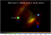 |
Fig. 2 WISE images (W2 = 4.6 μm in blue, W3 = 12 μm in green, andW4 = 22 μm in red) showing a bow-shock structure near HD 52382. The white arrow indicates the direction of the proper motion of the star. |
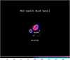 |
Fig. 3 WISE W1 and W4 images (3.4 μm and 22 μm, respectively) showing a double component or a wind-lobe structure. Yellow curves represent regions with the same brightness. |
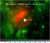 |
Fig. 4 WISEimages showing wind-blown and warm dust structures around HD 99953. |
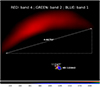 |
Fig. 5 Bow-shock structure and asymmetric density structure associated with HD 115842. The yellow curves represent regions withthe same brightness, each one associated with a different lobe. |
4.2 Global properties of stellar and wind parameters
Although the stars present spectral variability, it is still possible to describe their global properties. Figure 6 shows a comparison of Teff of BSGs with the spectral subtype. The sample is a collection of data from the literature and this work. With the exception of those stars that have Teff based on the BCD spectrophotometric calibration (Zorec et al. 2009), the effective temperature was obtained via adjustments of the line profiles of He I, He II, and line intensity ratio of Si IV/Si III or Si III/Si II, as in this work.
We performed a fit to the observed Teff versus spectral subtype relation using a third-order polynomial regression (a = −54.6 ± 7.7, b = 973.4 ± 107.5, c = −6054.3 ± 387.9, and d = 27 316 ± 331). The derived coefficients agree very well with the fit obtained by Markova & Puls (2008). We illustrate our fit in Fig. 6 with a grey wide band that has a dispersion of 1290 K. The supergiants of our sample, with the exception of HD 52089, HD 53138, and HD 47240 (indicated in the figure with large open circles), fall inside the traced relation. Moreover, we can observe that the departures of the effective temperatures for the early BSGs range roughly from 0 K to 5000 K and tend to be lower the later the B spectral subtype. This same tendency is also observed in Markova et al. (2008).
Figure 7 displays a linear correlation between log Teff and log gcor (the surface gravity corrected by the centrifugal acceleration, see Table A.1). This kind of correlation was previously reported by Searle et al. (2008). We performed a linear fit and obtained a slope of 3.98 ± 0.31. This indicates that most of the stars in our sample have a similar luminosity-to-mass ratio (log (L∕M) ~ 4), as expected, since  .
.
A large scatter is observed around the stars that have large log gcor (≥ 2.5); in particularHD 42087, HD 52089, and HD 64760 do not follow the relation. Two of these stars, HD 42087 and HD 64760, are close to the TAMS so we believe they have just left the main sequence. HD 64760 is a high rotator and, as a consequence, we should observe higher apparent bolometric luminosities and lower effective temperatures than those expected for their non-rotating stellar counterparts (Frémat et al. 2005; Zorec et al. 2005), giving a later evolutionary stage of the object.
From Table 3 we can distinguish stars showing two different wind regimes. One group gathers stars with steep velocity gradients, β ≤ 1, in good agreement with the standard wind theory, while the other group shows values of β between 1.5 and 3.3, similar to the results reported by Crowther et al. (2006), Searle et al. (2008), and Markova et al. (2008). Stars with β between 2 and 2.5 are the most common ones. High values of β are often found among the late B-type stars.
The terminal velocities range from 155 km s−1 to 1700 km s−1, while mass-loss rates range generally from 0.08 × 10⁻⁶ M⊙ yr−1 to 0.7 × 10⁻⁶ M⊙ yr−1 (four stars fall outside this mass-loss range).
In addition, we calculate the average values for the total mechanical momentum flow of the wind, Dmom, as a function of the luminosity of the star. This is known as the modified WLR (Kudritzki et al. 1995), given by
 (1)
(1)
where αeff = α − δ (see details in Kudritzki et al. 1999; Puls et al. 1996); α and δ are the force multipliers related to the line opacity and wind ionization, respectively.
Our sample splits into two different groups (see Fig. 8): the early BSGs with spectral types between B0 and B1.5 (blue diamonds) and mid- to late-type BSGs with spectral types from B2 to B9 (green and red diamonds). These two groups seem to be clearly separated. However, among the early B supergiants we found three mid B stars (HD 41117, HD 42087, and the variable star HD 99953) with wind momentum rates comparable to the early ones.
From a linear regression, we found that the sample of the early BSGs plus the three mentioned mid B stars (see Fig. 8, large circles) can be fitted by the following relationship:
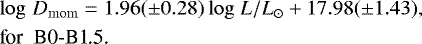 (2)
(2)
The second WLR was traced using BSG stars with spectral types B2-B9 (see Fig. 8, large triangles). The values of the wind momentum rates of these stars are clearly lower than those of the early-type objects. Furthermore, the WLR displays a different slope (less steep) with luminosity. For these objects we find a linear regresion of the form
 (3)
(3)
The observed offset between the WLRs increases from the early- to the mid-type BSGs. Despite the large errors of these quantities, the tendency is opposite to the results observed by Kudritzki et al. (1999) and predicted by Vink (2000).
In Fig. 8, observations of the same star at different epochs are connected by solid lines. For these stars, average values of log Dmom (Fig. 8, black dots) were considered to fit the regression line of the WLR for each group, i.e. early B or mid/late B stars. In thenext section, we return to the issue of mass-loss variations.
It is interesting to stress that the wind regime of the stars defining each WLR is different. From Table 3 we found that the early-type stars have mostly β < 2 and terminal velocities greater than 500 km s−1, while the mid- and late-type stars have β ≥ 2 and terminal velocities lower than 500 km s−1.
On the other hand, the parameter αeff, which is the inverse of the slope of the WLR, changes from 0.5 for the early BSGs to 0.7 for the mid/late ones. An increase in αeff might suggest highly structured ionized outflows that lead to a weakening of the radiation force. Under this condition, different mechanisms (e.g. pulsations, clumping) might also contribute to driving the wind.
Finally, Fig. 9 shows the ratios of V∞∕Vesc as a function of log Teff. In the figure we present our results together with the two temperature regions defined by Markova & Puls (2008), which show significantly different V∞∕Vesc ratios: 3.3 for effective temperatures above 23 000 K, and 1.3 below 18 000 K. Errors of 33% for the cooler and 43% for the hotter regions are shown as shaded areas (for details on the error determinations, see Markova & Puls 2008).
The region in between, delimited by vertical black lines, is called the bi-stability jump. Markova & Puls (2008) showed that the stars located there show a gradual decrease in V∞∕Vesc. Overall, our results show a similar behaviour to that reported by these authors. In particular, we found many stars in our sample located inside the bi-stability region. Moreover, as some stars are variable we also plotted in Fig. 9 the various positions of those stars observed during different epochs. These positions are connected with a solid black line.
The variation in V∞∕Vesc of those stars on the cool side of the bi-stability jump seems to be small. Instead, HD 99953 (green diamonds with triangles), which is located inside the bi-stability region, presents such a large wind variability that it seems to switch from a slow to a fast regime. The same variation for this star is observed in the WLR. With the exception of HD 80077, which has a huge mass-loss rate, we do not observe that a decrease in V∞∕Vesc is accompanied by an increase in the mass-loss rate, as predicted by Vink et al. (1999). In general, mid and late BSGs present values of Ṁ that are similar to or lower than those of the stars located on the hot side of the bi-stability jump.
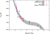 |
Fig. 6 Effective temperature as function of the spectral subtype. The relation was fitted using a third-order polynomial regression (dotted line) with a dispersion of 1290 K (grey band, see text for details). Comparison of our sample of Galactic B supergiants with a set of BSGs collected from the literature. Data points of our sample with large open circles are outliers. |
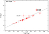 |
Fig. 7 Linearrelation (logTeff– log gcor) of our sample of B Galactic supergiants (dashed line). The surface gravity was corrected by the centrifugal acceleration. |
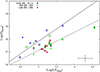 |
Fig. 8 Wind-momentum luminosity relationships (dotted lines). Blue, green, and red diamonds represent early-, mid-, and late-type BSGs, respectively. The upper fit line was derived using data points in large circles, while the lower fit line corresponds to data points with large triangles. Diamond symbols connected with solid lines correspond to observations of the same star in different epoch (black dots represent their average values). |
 |
Fig. 9 Ratiosof V∞∕Vesc as a functionof log Teff. Early-type (E), mid-type (M), and late-type (L) stars are indicated by blue, green, and red diamonds, respectively. Stars with wind variability are indicated with large open triangles and connected with a solid line. The largest variability is shown by HD 99953, which is located in the region limited by vertical black lines (the bi-stability jump). The shaded areas refer to two zones with different V∞ ∕Vesc: 3.3 for effective temperatures above 23 000 K, and 1.3 below 18 000 K, with errors of 43% and 33%, respectively, which were identified by Markova & Puls (2008). |
5 Discussion
5.1 Photospheric parameters
For some stars different estimates of Teff and log g (Δ Teff > 1500 K, and Δ log g ~ 0.2) are found inthe literature (see Table A.1).
In relation with these Teff estimates, itis important to point out that this parameter is derived using different methods or approaches. Quite often the atmosphericparameters are obtained by fitting the observed line profiles with a synthetic spectrum calculated from NLTE line-blanketed plane-parallel hydrostatic model atmospheres, using the codes TLUSTY and SYNSPEC (Hubeny & Lanz 1995; Lanz & Hubeny 2007). This procedure was mainly carried out by Fraser et al. (2010), McErlean et al. (1999), Kudritzki et al. (1999), while Crowther et al. (2006), Lefever et al. (2007), Markova & Puls (2008), Searle et al. (2008) used codes like FASTWIND or CMFGEN (Puls et al. 2005; Hillier & Miller 1998) that solve multi-level non-LTE radiative transfer problems in the co-moving frame, based on NLTE line-blanketed spherically symmetric wind models.
For most of the stars in our sample, we found good agreement between our Teff estimates and those obtained by Crowther et al. (2006, six stars in common), Lefever et al. (2007, eight stars in common), and Searle et al. (2008, five stars in common), within error margins of ± 1500 K. Good agreements were also found with the values derived by Fraser et al. (2010, twelve stars in common), who used TLUSTY. Among all the previous mentioned authors, the largest discrepancies in Teff are found for six stars, HD 42087, HD 52089, HD 53138, HD 64740, HD 92964, and HD 99953, which show appreciable differences (Δ Teff > 2000 K). Two of them (HD 53 138 and HD 64740) have shown either some degree of ion stratification or ionization changes in the UV lines (see details in Prinja et al. 2002). The star HD 52089 has a magnetic field and X-ray emission (see Sect. 4.1) and like HD 99953 is located inside the bi-stability region. This might suggest that these stars show intrinsic temperature variations since we do not observe a tendency regarding a particular method used to derive their atmospheric parameters.
We also found that the line spectra do not show He forbidden components suggesting that the He abundance is close to the solar value. This is in accordance with what Kraus et al. (2015) observed in 55 Cyg. In addition, Crowther et al. (2006) did not report any discrepancies on the Si and He abundances.
We did not find any correlation between Vmacro and Teff, as was reported by Fraser et al. (2010). In general, we needed larger values for Vmacro (mostly around 50−60 km s−1 for all the stars) than the ones given in the literature to be able to fit the photospheric line widths. In some cases it was even necessary to slightly increase V sin i as well. This could be due to our use of a mean value for Vmacro to model all the lines and, particularly, the line-forming region for He might extend into the base of the wind where higher turbulent velocities can be expected.
The major discrepancy found among the stellar parameters with previous works is related to the determination of the stellar radius, due to the different methods used to calculate distances to stars. We think that the values we estimated in Sect. 4.1 are quite reliable. Uncertainties in the stellar radius yield an insecure luminosity and a mass-loss discrepancy. This last issue is discussed in the next subsection.
5.2 Spectral and wind variability
Variable B supergiants often show spectroscopic variability in the optical and UV spectral region that can be attributed to the large-scale wind structures (Prinja et al. 2002). Variations linked to rotational modulation have been reported, for example, in HD 14134 and HD 64760 (Morel et al. 2004; Prinja et al. 2002, respectively), while those associated with pulsation activity were found in HD 50064 and 55 Cyg (Aerts et al. 2010; Kraus et al. 2015, respectively). Nevertheless, variability related to the presence of weak magnetic fields has also been proposed (Henrichs et al. 2003; Morel et al. 2004).
Most of the stars in our sample show Hα line variations in both shape and intensity. These variations can take place on a scale of a few days, but daily and even hourly variability has also been reported (e.g. Morel et al. 2004; Kraus et al. 2012, 2015; Tomić et al. 2015). Among our sample, HD 75149, HD 53138, and HD 111973 display emission-line episodes or dramatic line profile variations with a diversity of alternating shapes (from a pure absorption to a P Cygni profile and vice versa).
Regarding the amplitude of the mass-loss variation in individual objects, Prinja & Howarth (1986) measured a variability at 10% level on timescales of a day or longer, while Lefever et al. (2007) and Kraus et al. (2015) reported on ratios between maximum and minimum mass-loss rates ranging from 1.05 up to 2.5.
In this way, based on a carefully study of the variation in the Hα line among the stars we observed at different epochs (modelled with the code FASTWIND), the largest variations in Ṁ (a factor of 1.5 to 2.7) are detected in HD 75149, HD 99953, and HD 111973. As the Hα line is very sensitive to changes in the mass density and in the velocity gradients at the base of the wind (Cidale & Ringuelet 1993), a connection between line variability and changes in the wind structure due to photospheric instabilities can be expected.
To gain insight into the origin of the variability of the BSG winds, we gathered information from the literature for all our objects on periods of light and spectroscopic variations (quoted in Table 1), and on previous determinations of the wind parameters derived from individual modelling attempts. A comparison of the mass-loss estimates listed in Table A.1 is of particular interest as they displayratios between maximum and minimum values that range from 1 to 7. These discrepancies are not completely true because these models were computed using different stellar radii, and the differences in mass-loss rates could be much lower. For instance, for HD 34085 we found a discrepancy in Ṁ of 1.9 when compared with the result given by Markova & Puls (2008), but it could be only 1.3 times higher (Ṁ = 0.44 × 10⁻⁶ M⊙ yr−1) if a value of R⋆ = 115 R⊙ is adopted (keeping all the other parameters constant).
Therefore, to compare the values obtained by different authors we should discuss the scaling properties of the corresponding models since line fits are not unique (Puls et al. 2008). Thus we will adopt the optical-depth invariant Qr= Ṁ/ , instead of the traditional parameter Q = Ṁ/
 (Puls et al. 1996) since we assume that V∞ can change due to the wind variability. The corresponding calculations and errors for log Qr are given inTable A.1. An overview of these values shows that the differences in log Qr (for the stars we observed at different epochs) are two or three times larger than their corresponding error bars suggesting real variations in the wind parameters. These differences can also be observed among the Qr values we calculated from data given by different authors.
It is interesting to note that we found five stars in the domain of the bi-stability region. HD 99953 shows pronounced Hα variations from which different estimations of V∞ (250 km s−1, 500 km s−1, and 700 km s−1) and Ṁ (0.08 × 10⁻⁶ M⊙ yr−1, 0.13 × 10⁻⁶ M⊙ yr−1, and 0.22 × 10⁻⁶ M⊙ yr−1) were obtained. This implies variations in V∞ and Ṁ of a factor of about 2.8. This result goes against the theoretical prediction made by Vink et al. (1999) who argue that the jump in mass loss is accompanied by a steep decrease in the ratio V∞∕Vesc (from 2.6 to 1.3), which is close to the observed bi-stability jump in the terminal velocity. Moreover, these authors proposed that if the wind momentum Ṁ V∞ were about constant across the bi-stability jump, the mass-loss rate would have increased by a factor of two from stars with spectral types earlier than B1 to later than B1.
In the particular case of HD 99953, our result indicates that Ṁ V∞ is not constant (see Fig. 8) nor does the mass loss increases when the ratio V∞∕Vesc decreases, even when the observed changes in the variables are of the order of the expected values (~ 2.8). On the other hand, the mass loss derived for HD 99953 (log Ṁ = −6.66, when V∞= 700 km s−1) agrees with the value computed by Vink et al. (1999, − 6.54 for V∞∕Vesc = 2.6) in Table 1; however, the terminal velocity we derived is the half of the theoretical value found by these authors. We do not believe that the discrepancy could be due to the luminosity of the star (logL∕L⊙ = 4.87 ± 0.37) since the models were computed for a logL∕L⊙ = 5. We also found that this is not related to the velocity law adopted for the model since HD 47240 does not fit either.
Looking for other observed BSGs with logL∕L⊙~ 5 (see Table 1), we found that the wind parameters of the stars on the hot side of the bi-stability jump, like HD 38771 (with log Ṁ = −6.85 and V∞= 1500 km s−1) and HD 52382 (with log Ṁ = −6.62 and V∞= 1000 km s−1), resemble those listed in Table 1 by Vink et al. (1999). In contrast, the wind parameters of the stars on the cool side of the bi-stability jump, like HD 34085 (with log Ṁ = −6.64 and V∞∕Vesc = 0.8), HD 58350 (with log Ṁ = −6.82 and V∞∕Vesc = 0.9), and HD 111973 (with log Ṁ between − 6.7 and − 6.85, and V∞∕Vesc = 1.4) do not fit any model predictions. They often have lower terminal velocities and mass-loss rates than values expected from the models. This means that a decrease in the ratio V∞∕Vesc, both inside and on the cool side of the bi-stability jump, is not accompanied by an increase in the mass-loss rate. This result supports the conclusions drawn by Markova & Puls (2008) who used the modified optical depth invariant and found that both Ṁ and V∞ are decreasing in parallel.
We believe that the decrease in both the mass-loss rate and the terminal velocity, on the cool side of the bi-stability jump, could be explained with the δ-slow hydrodynamic solution for radiation line-driven winds (Curé et al. 2011). Venero et al. (2016) found that a change in the ionization of the wind, characterized by the parameter δ of the line-force multiplier (Abbott 1982), defines two different stationary wind regimes (fast and slow). The fast regime is always present at high effective temperatures (>25 000 K), while fast or slow regimes could develop at low effective temperatures. Both wind regimes are separated by an instability zone where non-stationary flow regimes exist. Venero et al. (2016) proposed that an initial density perturbation could trigger a switch in the wind regime between fast and slow solutions (and vice versa) in the B mid-type supergiants. In the same work the authors show preliminary computations of wind hydrodynamics using time-dependent wind solutions that lead to the formation of kink velocity field structures which might be related to the evolution of absorption components like the ones observed in the UV line spectrum (DACs). In addition, at temperatures <17 000 K the models predict a decrease in both terminal velocity and mass-loss rate (see Fig. 4 in Venero et al. 2016). Futher research on the slow hydrodynamics solution is in progress (Venero et al. 2017).
5.3 The wind momentum–luminosity relationship
The empirical WLR of massive stars is generally represented by a linear regression of the form
 (4)
(4)
Values for the coefficients X = 1∕αeff and D0 reported in the literature are given in Table 4, together with the parameter αeff and the corresponding errors. It is worth mentioning that previous investigations on the WLR for Galactic BSGs (see Table 4) show that wind momentum rates derived by means of line-blanketed analyses are systematically higher than those reported by Kudritzki et al. (1999).
The coefficients (X, D0) derived in this work for the early BSGs are close to those obtained by Herrero et al. (2002) and Mokiem et al. (2007), who used a sample of stars consisting mostly of OSGs. Both coefficients also agree with the theoretically predicted values of Vink (2000), but disagreewith the values obtained by Kudritzki et al. (1999) and Searle et al. (2008). These relations are plotted in Fig. 10.
Particularly, we find that the difference between our (X, D0) values and those of Searle et al. (2008) could be due to the fact that the sample of stars selected by these authors considered a mix of early and mid BSG types. In fact, if we split their sample, we obtain X = 1.85 ± 0.36 and D0 = 18.47 ± 2.00 for early BSGs, and X = 1.35 ± 0.14 and D0 = 21.08 ± 0.73 for the mid BSGs, which both agree with our values.
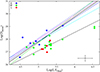 |
Fig. 10 Comparison of various empirical WLR: this work (solid and dashed black lines are for early BSGs and mid- or late-type BSGs, respectively), Herrero et al. (2002, solid green line), Searle et al. (2008, solid cyan line), and Mokiem et al. (2007, magenta solid line). The theoretical WLR of Vink (2000) is in blue, solid and dashed lines are for Teff > 27 500 K and Teff < 22 500 K, respectively. The figure includes the sample of stars shown in Fig. 8. |
5.4 The pulsation–mass-loss relationship
Saio (2011) demonstrated that one or more radial strange modes are expected to be excited in evolved BSGs. These authors computed the periods of excited modes during the evolution of only two stellar models: stars with initial masses of 20 M⊙ and 25 M⊙. It appears that the periods of these radial strange modes tend to decrease when the effective temperature of the star increases during the blue-ward evolution.
As radial strange modes are considered suitable to trigger mass loss, we first checked which of the known (photometric and spectroscopic) periods (see Table 1) might be considered as radial strange modes, and then opted for a comparison of these periods with the amplitude of the mass-loss rates (i.e. ratios between maximum and minimum values) using the Qr parameters given in Table A.1.
According to the models of Saio et al. (2013), the radial modes, especially in late-type stars, display the longest periods. Therefore, for each star we searched for correlations with the longest known period. As shown in Fig. 11, we found a linear correlation for stars mostly represented by mid/late BSGs (i.e. spectral type from B2 to B9) with P > 6 days. The longer the period the lower the amplitude of the parameter Qr. We added to our sample two well-studied variable stars having measurements of their stellar and wind parameters (Deneb and 55 Cyg, Scuderi et al. 1992; Chesneau et al. 2010; Kraus et al. 2015). Three mid-type BSGs with measured values of P and Ṁ were rejected from the sample: HD 53138, HD 75149, and HD 99953 (Fig. 11, green dots without triangles). Two of these stars HD 75149 and HD 99953 have been poorly studied and new periods should probably be determined. The former, in particular, might have inaccurate minimum values of Ṁ since two of our observed profiles are in absorption. The star HD 111973 is not included since we have observations during an interval of time of two days which is less than the reported period of variation.
The relationship we obtained is Pmax = 100.27 (±7.64) X + 83.97(±4.47), where X =  , and was derived using the data enclosed in triangles (the used values of
  and
and  are listed in bold in Table A.1). The differences in the selected values are two or three times larger than their corresponding error bars, suggesting real variations in the mass-loss rates.
The group that comprises the early BSGs (HD 38771, the binary star HD 47420, HD 52089, HD 64760, and HD 148688, blue diamonds) does not show a clear correlation with their periods. Some of these stars show differences in their Qr parameters of the order of the errors suggesting that they do not show strong wind variability.
We canthen conclude that as the observed line profiles can be matched using a velocity β-law, radiation pressure is the main mechanism that drives the wind. However, pulsation modes may also play a significant role in (quasi-)periodically lifting the material, which will then be accelerated outwards by radiation. In this way, radial strange-mode pulsation with periods >6 days might be responsible for the wind variability in mid- and late-type BSGs.
Coefficient for the WLR derived by different authors.
 |
Fig. 11 Ratios between minimum and maximum Qr values as a function of the longest photometric/spectroscopic period, where |
5.5 Location of the BSGs in the HR diagram
Figure 12 displays the position of our sample stars in the HR diagram, using data from Table 3, together with the stability boundaries for the different pulsation modes, as defined by Saio et al. (2013). The stability boundary for low-order radial and non-radial p modes is represented by the blue solid line. This bends and becomes horizontal due to strange-mode instability which occurs when log L∕M > 4. Non-radial modes (low-degree high-order g-modes) can be excited in the region delimited by red lines, whilst monotonically unstable modes exist above the magenta dotted line in the most luminous part of the HR diagram (as is the case for the hypergiant star HD 80077). On the other hand, two stars in our sample (HD 52089 and HD 64760, with log L∕L⊙ < 4.6, log L∕M < 4) are located inside the instability strip of the β Cep, found by Saio et al. (2013) and Georgy et al. (2014), near the cool border of that region. Particularly, HD 64740 presents in the UV spectral region clear signs of phase bowing and ionization changes in the wind that could be associated with strong shocks originating in the interface between slow and fast wind streams, such as in a model of co-rotating interaction regions (Prinja et al. 2002), and its WISE image reveals a kind of wind-lobe structure. We propose that this star could be evolving towards the RSG stage.
In the same HR diagram we can also see that the mid-/late-type stars are located in the region where oscillatory convection modes would be observable (cyan lines, Saio 2011; Saio et al. 2013), with the exception of HD 41117 and HD 99953, which are located together with the early B types. The star 55 Cyg (taken from Kraus et al. 2015) was also included.
It is worth mentioning that WISE images reveal signs of previous strong wind-ISM interaction in three objects in our sample (HD 52382, HD 99953, and HD 115842) pointing out that these stars could be evolving towards the blue-loop after a post-RSG phase. This same also holds true for 55 Cyg (Kraus et al. 2015).
 |
Fig. 12 Position of the sample of stars in the HR diagram. Evolutionary tracks (taken from Ekström et al. 2012, black solid lines) correspond to non-rotating stars with M⋆ = 12, 15, 20, 32, 40, and 60 M⊙. The coloured curves define instability boundaries of various modes (Saio 2011): a) stability boundary for low-order radial and non-radial p modes (blue solid line); b) non-radial g modes with l = 1 and 2 (red short-dashed and solid lines, respectively); c) oscillatory convection modes (cyan dot-dashed lines); d) monotonically unstable radial modes (above the magenta dotted-line, where the hypergiant star HD 80077 is found). The blue, green, red, and magenta diamonds correspond to early (E), mid (M), and late (L) BSGs, and 55 Cyg, respectively. |
6 Conclusions
We studied a sample of 19 Galactic BSGs by fitting theoretical line profiles of H, He, and Si to the observed profiles. The synthetic line profiles were computed with the NLTE atmosphere code FASTWIND to obtain new estimates for their stellar and wind parameters. The mass-loss rates for HD 74371, HD 99953, and HD 111973 have been derived for the first time. In addition, some BSGs in our sample show short-term variability in the Hα and UV resonance lines, indicating important changes in the wind structure.
In relation with the global properties of the stellar winds of our sample, we find two different behaviours in the WLR. The early and mid B-type stars have mostly β < 2 and terminal velocities greater than 500 km s−1, while the other group is comprised mostly by mid and late B-type stars with β ≥ 2 and terminal velocities lower than 500 km s−1. In addition, we find that the coefficients for the linear regression of early BSGs agree with theoretical or empirical values found by Vink (2000), Herrero et al. (2002), Mokiem et al. (2007). As well, our coefficients would agree with data from Searle et al. (2008) if we separated their sample of stars into two groups: early and mid BSGs.
Furthermore, we observe that a decrease in the ratio V∞∕Vesc in the bi-stability region, and on its cool side, is accompanied by a decrease in mass-loss rate. This observation is contrary to the theoretical result obtained by Vink et al. (1999), based on a fast wind regime. Instead, this behaviour seems to be consistent with predictions from highly ionized stellar winds (δ-slow solution, Venero et al. 2016). The possible switch between fast and δ-slow solutions should be explored in detail.
Finally, we found an empirical correlation (period–mass-loss relationship) that associates the amplitude of the mass-loss variations with long-term photometric and/or spectroscopic variability. This relation is expressed in terms of the Qr parameter. The found period–mass-loss relationship could indicate that radial (or strange) pulsation modes with periods >6 days are related to the wind variability. To confirm this trend, it is necessary to perform long-term high-resolution spectroscopic campaigns to properly measure oscillation periods and simultaneously derive homogeneous sets of mass-loss rates.
Acknowledgements
We thanks our anonymous referee for the helpful comments and suggestions. We also want to acknowledge J. Puls for allowing us to use the FASTWIND code, for his help and advice with the code, and for the fruitful suggestions. This research has also made use of the SIMBAD database, operated at CDS, Strasbourg, France, and the International Variable Star Index (VSX) database, operated at AAVSO, Cambridge, Massachusetts, USA. L.C. and M.C. acknowledge support from the project CONICYT + PAI/Atracción de capital humano avanzado del extranjero (folio PAI80160057). L.C. also acknowledges financial support from CONICET (PIP 0177), La Agencia Nacional de Promoción Científica y Tecnológica (PICT 2016-1971) and the Programa de Incentivos (G11/137) of the Universidad Nacional de La Plata (UNLP), Argentina. R.V. is grateful for the finantial support from the UNLP under programme PPID/G003. M.C., S.K., and C.A. acknowledge support from Centro de Astrofísica de Valparaíso. C.A. also thanks BECAS DE DOCTORADO NACIONAL CONICYT 2016-2017. M.K. acknowledges support from GAČR (17-02337S). The Astronomical Institute Ondřejov is supported by the project RVO:67985815. This work was partly supported by the European Union European Regional Development Fund, project “Benefits for EstonianSociety from Space Research and Application” (KOMEET, 2014 – 2020. 4. 01. 16 - 0029), and by the institutional research funding IUT40 − 1 of the Estonian Ministry of Education and Research. Financial support for International Cooperation of the Czech Republic and Argentina (AVCR-CONICET/14/003) is acknowledged.
Appendix A Photospheric line-fitting and compiled data from the literature
The following figures present a comparison between observed and synthetic photospheric line profiles calculated with FASTWIND and the parameters quoted in Table 3. These parameters are also given in Table A.1 together with a set of stellar and wind parameters gathered from the literature.
Stellar and wind parameters.
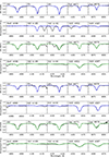 |
Fig. A.1 HD 34085, HD 38771, HD 41117, and HD 47240: Line model fittings to observations. |
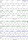 |
Fig. A.2 HD 42087, HD 52089, HD 52382, and HD 53138: Line model fittings to observations. |
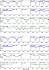 |
Fig. A.3 HD 53138, HD 58350, and HD 64760: Line model fittings to observations. |
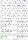 |
Fig. A.4 HD 74371 and HD 75149: Line model fittings to observations. |
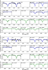 |
Fig. A.5 HD 75149, HD 79186, HD 92964, and HD 80077: Line model fittings to observations. |
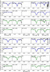 |
Fig. A.6 HD 99953 and HD 111973: Line model fittings to observations. |
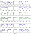 |
Fig. A.7 HD 111973, HD 115842, and HD 148688: Line model fittings to observations. |
References
- Abbott, D. C. 1982, ApJ, 259, 282 [NASA ADS] [CrossRef] [Google Scholar]
- Aerts, C., Lefever, K., Baglin, A., et al. 2010, A&A, 513, L11 [NASA ADS] [CrossRef] [EDP Sciences] [Google Scholar]
- Aerts, C., Simón-Díaz, S., Catala, C., et al. 2013, A&A, 557, A114 [NASA ADS] [CrossRef] [EDP Sciences] [Google Scholar]
- Astraatmadja, T. L., & Bailer-Jones, C. A. L. 2016, ApJ, 833, 119 [NASA ADS] [CrossRef] [Google Scholar]
- Barlow, M. J., & Cohen, M. 1977, ApJ, 213, 737 [NASA ADS] [CrossRef] [Google Scholar]
- Benaglia, P., Vink, J. S., Martí, J., et al. 2007, A&A, 467, 1265 [NASA ADS] [CrossRef] [EDP Sciences] [Google Scholar]
- Bouret, J.-C., Lanz, T., & Hillier, D. J. 2005, A&A, 438, 301 [NASA ADS] [CrossRef] [EDP Sciences] [Google Scholar]
- Carpay, J., de Jager, C., Nieuwenhuijzen, H., & Moffat, A. 1989, A&A, 216, 143 [NASA ADS] [Google Scholar]
- Carpay, J., de Jager, C., & Nieuwenhuijzen, H. 1991, A&A, 248, 475 [NASA ADS] [Google Scholar]
- Castor, J. I., Abbott, D. C., & Klein, R. I. 1975, ApJ, 195, 157 [NASA ADS] [CrossRef] [Google Scholar]
- Chesneau, O., Dessart, L., Mourard, D., et al. 2010, A&A, 521, A5 [NASA ADS] [CrossRef] [EDP Sciences] [Google Scholar]
- Chesneau, O., Kaufer, A., Stahl, O., et al. 2014, A&A, 566, A125 [NASA ADS] [CrossRef] [EDP Sciences] [Google Scholar]
- Chini, R., Hoffmeister, V. H., Nasseri, A., Stahl, O., & Zinnecker, H. 2012, MNRAS, 424, 1925 [NASA ADS] [CrossRef] [Google Scholar]
- Cidale, L. S., & Ringuelet, A. E. 1993, ApJ, 411, 874 [NASA ADS] [CrossRef] [Google Scholar]
- Cohen, D. H., Cooper, R. G., Macfarlane, J. J., et al. 1996, ApJ, 460, 506 [NASA ADS] [CrossRef] [Google Scholar]
- Crowther, P. A., Lennon, D. J., & Walborn, N. R. 2006, A&A, 446, 279 [NASA ADS] [CrossRef] [EDP Sciences] [Google Scholar]
- Curé, M., Cidale, L., & Granada, A. 2011, ApJ, 737, 18 [NASA ADS] [CrossRef] [Google Scholar]
- Ebbets, D. 1982, ApJS, 48, 399 [NASA ADS] [CrossRef] [Google Scholar]
- Ekström, S., Georgy, C., Eggenberger, P., et al. 2012, A&A, 537, A146 [NASA ADS] [CrossRef] [EDP Sciences] [Google Scholar]
- Evans, C. J., Lennon, D. J., Trundle, C., Heap, S. R., & Lindler, D. J. 2004, ApJ, 607, 451 [NASA ADS] [CrossRef] [Google Scholar]
- Feldmeier, A. 1998, A&A, 332, 245 [NASA ADS] [Google Scholar]
- Firnstein, M., & Przybilla, N. 2012, A&A, 543, A80 [NASA ADS] [CrossRef] [EDP Sciences] [Google Scholar]
- Flower, P. J. 1996, ApJ, 469, 355 [NASA ADS] [CrossRef] [Google Scholar]
- Fraser, M., Dufton, P. L., Hunter, I., & Ryans, R. S. I. 2010, MNRAS, 404, 1306 [NASA ADS] [Google Scholar]
- Frémat, Y., Zorec, J., Hubert, A., & Floquet, M. 2005, A&A, 440, 305 [NASA ADS] [CrossRef] [EDP Sciences] [Google Scholar]
- Friend, D. B., & Abbott, D. C. 1986, ApJ, 311, 701 [NASA ADS] [CrossRef] [Google Scholar]
- Fullerton, A. W., Massa, D. L., & Prinja, R. K. 2006, ApJ, 637, 1025 [NASA ADS] [CrossRef] [Google Scholar]
- Garcia, M., Herrero, A., Najarro, F., et al. 2017, IAU Symp., 329, 313 [NASA ADS] [Google Scholar]
- Garmany, C. D., Olson, G. L., van Steenberg, M. E., & Conti, P. S. 1981, ApJ, 250, 660 [NASA ADS] [CrossRef] [Google Scholar]
- Gathier, R., Lamers, H. J. G. L. M., & Snow, T. P. 1981, ApJ, 247, 173 [NASA ADS] [CrossRef] [Google Scholar]
- Georgy, C., Saio, H., & Meynet, G. 2014, MNRAS, 439, L6 [NASA ADS] [CrossRef] [Google Scholar]
- Glatzel, W., Kiriakidis, M., Chernigovskij, S., & Fricke, K. J. 1999, MNRAS, 303, 116 [NASA ADS] [CrossRef] [Google Scholar]
- Godart, M., Simón-Díaz, S., Herrero, A., et al. 2017, A&A, 597, A23 [NASA ADS] [CrossRef] [EDP Sciences] [Google Scholar]
- Grevesse, N., & Sauval, A. J. 1998, Space Sci. Rev., 85, 161 [NASA ADS] [CrossRef] [Google Scholar]
- Henrichs, H. F., Neiner, C., & Geers, V. C. 2003, in A Massive Star Odyssey: From Main Sequence to Supernova, eds. K. van der Hucht, A. Herrero, & C. Esteban, IAU Symp., 212, 202 [NASA ADS] [Google Scholar]
- Herrero, A., Puls, J., & Najarro, F. 2002, A&A, 396, 949 [NASA ADS] [CrossRef] [EDP Sciences] [Google Scholar]
- Hillier, D. J., & Miller, D. L. 1998, ApJ, 496, 407 [NASA ADS] [CrossRef] [Google Scholar]
- Hoffleit, D., & Jaschek, C. 1991, The Bright Star Catalogue (New Haven: Yale University Observatory) [Google Scholar]
- Howarth, I. D., Siebert, K. W., Hussain, G. A. J., & Prinja, R. K. 1997, MNRAS, 284, 265 [NASA ADS] [CrossRef] [Google Scholar]
- Hubeny, I., & Lanz, T. 1995, ApJ, 439, 875 [Google Scholar]
- Humphreys, R. M. 1978, ApJS, 38, 309 [NASA ADS] [CrossRef] [EDP Sciences] [Google Scholar]
- Israelian, G., Chentsov, E., & Musaev, F. 1997, MNRAS, 290, 521 [NASA ADS] [CrossRef] [Google Scholar]
- Jaschek, M., & Brandi, E. 1973, PASP, 85, 736 [NASA ADS] [CrossRef] [Google Scholar]
- Kaufer, A., Stahl, O., Prinja, R. K., & Witherick, D. 2006, A&A, 447, 325 [NASA ADS] [CrossRef] [EDP Sciences] [Google Scholar]
- Knoechel, G., & Moffat, A. F. J. 1982, A&A, 110, 263 [NASA ADS] [Google Scholar]
- Koen, C., & Eyer, L. 2002, MNRAS, 331, 45 [NASA ADS] [CrossRef] [Google Scholar]
- Kraus, M., Tomić, S., Oksala, M. E., & Smole, M. 2012, A&A, 542, L32 [NASA ADS] [CrossRef] [EDP Sciences] [Google Scholar]
- Kraus, M., Haucke, M., Cidale, L. S., et al. 2015, A&A, 581, A75 [NASA ADS] [CrossRef] [EDP Sciences] [Google Scholar]
- Krtička, J., & Kubát, J. 2001, A&A, 377, 175 [Google Scholar]
- Kudritzki, R.-P., Lennon, D. J., & Puls, J. 1995, in Science with the VLT, eds. J. R. Walsh & I. J. Danziger, 246 [Google Scholar]
- Kudritzki, R. P., Puls, J., Lennon, D. J., et al. 1999, A&A, 350, 970 [Google Scholar]
- Kurucz, R. L. 1979, ApJS, 40, 1 [NASA ADS] [CrossRef] [Google Scholar]
- Lamers, H. J. G. L. M., Gathier, R., & Snow, Jr. T. P. 1982, ApJ, 258, 186 [NASA ADS] [CrossRef] [Google Scholar]
- Lamers, H. J. G. L. M., Snow, T. P., & Lindholm, D. M. 1995, ApJ, 455, 269 [NASA ADS] [CrossRef] [Google Scholar]
- Lanz, T., & Hubeny, I. 2007, ApJS, 169, 83 [CrossRef] [Google Scholar]
- Lefever, K., Puls, J., & Aerts, C. 2007, A&A, 463, 1093 [NASA ADS] [CrossRef] [EDP Sciences] [Google Scholar]
- Lefever, K., Puls, J., Morel, T., et al. 2010, A&A, 515, A74 [NASA ADS] [CrossRef] [EDP Sciences] [Google Scholar]
- Lefèvre, L., Marchenko, S. V., Moffat, A. F. J., & Acker, A. 2009, A&A, 507, 1141 [NASA ADS] [CrossRef] [EDP Sciences] [Google Scholar]
- Marco, A., & Negueruela, I. 2009, A&A, 493, 79 [NASA ADS] [CrossRef] [EDP Sciences] [Google Scholar]
- Markova, N., & Puls, J. 2008, A&A, 478, 823 [NASA ADS] [CrossRef] [EDP Sciences] [Google Scholar]
- Markova, N., Puls, J., Repolust, T., & Markov, H. 2004, A&A, 413, 693 [NASA ADS] [CrossRef] [EDP Sciences] [Google Scholar]
- Markova, N., Prinja, R. K., Markov, H., et al. 2008, A&A, 487, 211 [NASA ADS] [CrossRef] [EDP Sciences] [Google Scholar]
- Massa, D., Fullerton, A. W., Nichols, J. S., et al. 1995, ApJ, 452, L53 [NASA ADS] [Google Scholar]
- McErlean, N. D., Lennon, D. J., & Dufton, P. L. 1999, A&A, 349, 553 [NASA ADS] [Google Scholar]
- Megier, A., Strobel, A., Galazutdinov, G. A., & Krełowski, J. 2009, A&A, 507, 833 [NASA ADS] [CrossRef] [EDP Sciences] [Google Scholar]
- Meynet, G., Maeder, A., Schaller, G., Schaerer, D., & Charbonnel, C. 1994, A&AS, 103, 97 [Google Scholar]
- Mokiem, M. R., de Koter, A., Vink, J. S., et al. 2007, A&A, 473, 603 [NASA ADS] [CrossRef] [EDP Sciences] [Google Scholar]
- Moravveji, E., Guinan, E. F., Shultz, M., Williamson, M. H., & Moya, A. 2012, ApJ, 747, 108 [NASA ADS] [CrossRef] [Google Scholar]
- Morel, T., Marchenko, S. V., Pati, A. K., et al. 2004, MNRAS, 351, 552 [NASA ADS] [CrossRef] [Google Scholar]
- Morel, T., Hubrig, S., & Briquet, M. 2008, A&A, 481, 453 [NASA ADS] [CrossRef] [EDP Sciences] [Google Scholar]
- Nerney, S. 1980, ApJ, 242, 723 [NASA ADS] [CrossRef] [Google Scholar]
- Oskinova, L. M., Hamann, W.-R., & Feldmeier, A. 2007, A&A, 476, 1331 [NASA ADS] [CrossRef] [EDP Sciences] [Google Scholar]
- Owocki, S. P., & Rybicki, G. B. 1984, ApJ, 284, 337 [NASA ADS] [CrossRef] [Google Scholar]
- Owocki, S. P., Castor, J. I., & Rybicki, G. B. 1988, ApJ, 335, 914 [NASA ADS] [CrossRef] [Google Scholar]
- Pasinetti Fracassini, L. E., Pastori, L., Covino, S., & Pozzi, A. 2001, A&A, 367, 521 [NASA ADS] [CrossRef] [EDP Sciences] [Google Scholar]
- Pauldrach, A. W. A., & Puls, J. 1990, A&A, 237, 409 [NASA ADS] [Google Scholar]
- Pauldrach, A., Puls, J., & Kudritzki, R. P. 1986, A&A, 164, 86 [NASA ADS] [Google Scholar]
- Peri, C. S., Benaglia, P., Brookes, D. P., Stevens, I. R., & Isequilla, N. L. 2012, A&A, 538, A108 [NASA ADS] [CrossRef] [EDP Sciences] [Google Scholar]
- Petrov, B., Vink, J. S., & Gräfener, G. 2014, A&A, 565, A62 [NASA ADS] [CrossRef] [EDP Sciences] [Google Scholar]
- Prinja, R. K., & Howarth, I. D. 1986, ApJS, 61, 357 [NASA ADS] [CrossRef] [Google Scholar]
- Prinja, R. K., & Massa, D. L. 2010, A&A, 521, L55 [Google Scholar]
- Prinja, R. K., & Massa, D. L. 2013, A&A, 559, A15 [NASA ADS] [CrossRef] [EDP Sciences] [Google Scholar]
- Prinja, R. K., Barlow, M. J., & Howarth, I. D. 1990, ApJ, 361, 607 [NASA ADS] [CrossRef] [Google Scholar]
- Prinja, R. K., Massa, D., & Fullerton, A. W. 1995, ApJ, 452, L61 [NASA ADS] [CrossRef] [Google Scholar]
- Prinja, R. K., Massa, D., Howarth, I. D., & Fullerton, A. W. 1998, MNRAS, 301, 926 [NASA ADS] [CrossRef] [Google Scholar]
- Prinja, R. K., Massa, D., & Fullerton, A. W. 2002, A&A, 388, 587 [NASA ADS] [CrossRef] [EDP Sciences] [Google Scholar]
- Prinja, R. K., Rivinius, T., Stahl, O., et al. 2004, A&A, 418, 727 [NASA ADS] [CrossRef] [EDP Sciences] [Google Scholar]
- Prugniel, P., Vauglin, I., & Koleva, M. 2011, A&A, 531, A165 [NASA ADS] [CrossRef] [EDP Sciences] [Google Scholar]
- Przybilla, N., Butler, K., Becker, S. R., & Kudritzki, R. P. 2006, A&A, 445, 1099 [NASA ADS] [CrossRef] [EDP Sciences] [Google Scholar]
- Puls, J. 1991, A&A, 248, 581 [NASA ADS] [Google Scholar]
- Puls, J., Kudritzki, R.-P., Herrero, A., et al. 1996, A&A, 305, 171 [NASA ADS] [Google Scholar]
- Puls, J., Urbaneja, M. A., Venero, R., et al. 2005, A&A, 435, 669 [NASA ADS] [CrossRef] [EDP Sciences] [Google Scholar]
- Puls, J., Vink,J. S., & Najarro, F. 2008, A&ARv, 16, 209 [NASA ADS] [CrossRef] [EDP Sciences] [Google Scholar]
- Rivero González, J. G., Puls, J., Najarro, F., & Brott, I. 2012, A&A, 537, A79 [NASA ADS] [CrossRef] [EDP Sciences] [Google Scholar]
- Rusconi, L., Sedmak, G., Stalio, R., & Arpigny, C. 1980, A&AS, 42, 347 [NASA ADS] [Google Scholar]
- Saio, H. 2011, MNRAS, 412, 1814 [NASA ADS] [CrossRef] [Google Scholar]
- Saio, H., Kuschnig, R., Gautschy, A., et al. 2006, ApJ, 650, 1111 [NASA ADS] [CrossRef] [Google Scholar]
- Saio, H., Georgy, C., & Meynet, G. 2013, MNRAS, 433, 1246 [NASA ADS] [CrossRef] [Google Scholar]
- Santolaya-Rey, A. E., Puls, J., & Herrero, A. 1997, A&A, 323, 488 [NASA ADS] [Google Scholar]
- Scuderi, S., Bonanno, G., di Benedetto, R., Spadaro, D., & Panagia, N. 1992, ApJ, 392, 201 [NASA ADS] [CrossRef] [Google Scholar]
- Scuderi, S., Panagia, N., Stanghellini, C., Trigilio, C., & Umana, G. 1998, A&A, 332, 251 [NASA ADS] [Google Scholar]
- Searle, S. C., Prinja, R. K., Massa, D., & Ryans, R. 2008, A&A, 481, 777 [NASA ADS] [CrossRef] [EDP Sciences] [Google Scholar]
- Simón-Díaz, S., & Herrero, A. 2007, A&A, 468, 1063 [NASA ADS] [CrossRef] [EDP Sciences] [Google Scholar]
- Simón-Díaz, S., & Herrero, A. 2014, A&A, 562, A135 [NASA ADS] [CrossRef] [EDP Sciences] [Google Scholar]
- Sterken, C. 1977, A&A, 57, 361 [NASA ADS] [Google Scholar]
- Sundqvist, J. O., Puls, J., & Feldmeier, A. 2010, A&A, 510, A11 [NASA ADS] [CrossRef] [EDP Sciences] [Google Scholar]
- Sundqvist, J. O., Puls, J., Feldmeier, A., & Owocki, S. P. 2011, A&A, 528, A64 [NASA ADS] [CrossRef] [EDP Sciences] [Google Scholar]
- Šurlan, B., Hamann, W.-R., Aret, A., et al. 2013, A&A, 559, A130 [NASA ADS] [CrossRef] [EDP Sciences] [Google Scholar]
- Tomić, S., Kraus, M., & Oksala, M. E. 2015, New Windows on Massive Stars, eds. G. Meynet, C. Georgy, J. Groh, & P. Stee, IAU Symp., 307, 235 [NASA ADS] [Google Scholar]
- Underhill, A. B. 1984, ApJ, 285, 668 [NASA ADS] [CrossRef] [Google Scholar]
- van Breda, I. G., Glass, I. S., & Whittet, D. C. B. 1974, MNRAS, 168, 551 [NASA ADS] [CrossRef] [Google Scholar]
- van Genderen, A. M., Bovenschen, H., Engelsman, E. C., et al. 1989, A&AS, 79, 263 [NASA ADS] [Google Scholar]
- van Leeuwen, F. 2007, A&A, 474, 653 [NASA ADS] [CrossRef] [EDP Sciences] [Google Scholar]
- van Leeuwen, F., van Genderen, A. M., & Zegelaar, I. 1998, A&AS, 128, 117 [NASA ADS] [CrossRef] [EDP Sciences] [Google Scholar]
- Venero, R. O. J., Curé, M., Cidale, L. S., & Araya, I. 2016, ApJ, 822, 28 [NASA ADS] [CrossRef] [Google Scholar]
- Venero, R. O. J., Cidale, L. S., Cure, M., & Haucke, M. 2017, Boletín de la Asociación Argentina de Astronomía, 59, 28 [NASA ADS] [Google Scholar]
- Vink, J. S. 2000, PhD Thesis, Universiteit Utrecht, The Netherlands [Google Scholar]
- Vink, J. S., de Koter, A., & Lamers, H. J. G. L. M. 1999, A&A, 350, 181 [NASA ADS] [Google Scholar]
- Vink, J. S., de Koter, A., & Lamers, H. J. G. L. M. 2001, A&A, 369, 574 [NASA ADS] [CrossRef] [EDP Sciences] [Google Scholar]
- Wenger, M., Ochsenbein, F., Egret, D., et al. 2000, A&AS, 143, 9 [NASA ADS] [CrossRef] [EDP Sciences] [Google Scholar]
- Woosley, S. E., Heger, A., & Weaver, T. A. 2002, Rev. Mod. Phys., 74, 1015 [NASA ADS] [CrossRef] [Google Scholar]
- Wright, E. L., Eisenhardt, P. R. M., Mainzer, A. K., et al. 2010, AJ, 140, 1868 [NASA ADS] [CrossRef] [Google Scholar]
- Yadav, A. P., & Glatzel, W. 2016, MNRAS, 457, 4330 [NASA ADS] [CrossRef] [Google Scholar]
- Zorec, J., Frémat, Y., & Cidale, L. 2005, A&A, 441, 235 [NASA ADS] [CrossRef] [EDP Sciences] [Google Scholar]
- Zorec, J., Cidale, L., Arias, M. L., et al. 2009, A&A, 501, 297 [NASA ADS] [CrossRef] [EDP Sciences] [Google Scholar]
IRAF is distributed by the National Optical Astronomy Observatory, which is operated by the Association of Universities for Research in Astronomy (AURA) under cooperative agreement with the National Science Foundation.
The Be Stars Observation Survey (BeSOS; http://besos.ifa.uv.cl) is a database containing reduced spectra acquired using the echelle spectrograph PUCHEROS.
All Tables
Stellar parameters calculated in the present study or adopted from the literature.
All Figures
|
Fig. 1 Hα line and the best-fitting synthetic model. For HD 53138, HD 58350, HD 75149, HD 80077, HD 99953, and HD 111973 more than one plot are shown due to multi-epoch observations. |
| In the text | |
|
Fig. 2 WISE images (W2 = 4.6 μm in blue, W3 = 12 μm in green, andW4 = 22 μm in red) showing a bow-shock structure near HD 52382. The white arrow indicates the direction of the proper motion of the star. |
| In the text | |
|
Fig. 3 WISE W1 and W4 images (3.4 μm and 22 μm, respectively) showing a double component or a wind-lobe structure. Yellow curves represent regions with the same brightness. |
| In the text | |
|
Fig. 4 WISEimages showing wind-blown and warm dust structures around HD 99953. |
| In the text | |
|
Fig. 5 Bow-shock structure and asymmetric density structure associated with HD 115842. The yellow curves represent regions withthe same brightness, each one associated with a different lobe. |
| In the text | |
|
Fig. 6 Effective temperature as function of the spectral subtype. The relation was fitted using a third-order polynomial regression (dotted line) with a dispersion of 1290 K (grey band, see text for details). Comparison of our sample of Galactic B supergiants with a set of BSGs collected from the literature. Data points of our sample with large open circles are outliers. |
| In the text | |
|
Fig. 7 Linearrelation (logTeff– log gcor) of our sample of B Galactic supergiants (dashed line). The surface gravity was corrected by the centrifugal acceleration. |
| In the text | |
|
Fig. 8 Wind-momentum luminosity relationships (dotted lines). Blue, green, and red diamonds represent early-, mid-, and late-type BSGs, respectively. The upper fit line was derived using data points in large circles, while the lower fit line corresponds to data points with large triangles. Diamond symbols connected with solid lines correspond to observations of the same star in different epoch (black dots represent their average values). |
| In the text | |
|
Fig. 9 Ratiosof V∞∕Vesc as a functionof log Teff. Early-type (E), mid-type (M), and late-type (L) stars are indicated by blue, green, and red diamonds, respectively. Stars with wind variability are indicated with large open triangles and connected with a solid line. The largest variability is shown by HD 99953, which is located in the region limited by vertical black lines (the bi-stability jump). The shaded areas refer to two zones with different V∞ ∕Vesc: 3.3 for effective temperatures above 23 000 K, and 1.3 below 18 000 K, with errors of 43% and 33%, respectively, which were identified by Markova & Puls (2008). |
| In the text | |
|
Fig. 10 Comparison of various empirical WLR: this work (solid and dashed black lines are for early BSGs and mid- or late-type BSGs, respectively), Herrero et al. (2002, solid green line), Searle et al. (2008, solid cyan line), and Mokiem et al. (2007, magenta solid line). The theoretical WLR of Vink (2000) is in blue, solid and dashed lines are for Teff > 27 500 K and Teff < 22 500 K, respectively. The figure includes the sample of stars shown in Fig. 8. |
| In the text | |
|
Fig. 11 Ratios between minimum and maximum Qr values as a function of the longest photometric/spectroscopic period, where |
| In the text | |
|
Fig. 12 Position of the sample of stars in the HR diagram. Evolutionary tracks (taken from Ekström et al. 2012, black solid lines) correspond to non-rotating stars with M⋆ = 12, 15, 20, 32, 40, and 60 M⊙. The coloured curves define instability boundaries of various modes (Saio 2011): a) stability boundary for low-order radial and non-radial p modes (blue solid line); b) non-radial g modes with l = 1 and 2 (red short-dashed and solid lines, respectively); c) oscillatory convection modes (cyan dot-dashed lines); d) monotonically unstable radial modes (above the magenta dotted-line, where the hypergiant star HD 80077 is found). The blue, green, red, and magenta diamonds correspond to early (E), mid (M), and late (L) BSGs, and 55 Cyg, respectively. |
| In the text | |
|
Fig. A.1 HD 34085, HD 38771, HD 41117, and HD 47240: Line model fittings to observations. |
| In the text | |
|
Fig. A.2 HD 42087, HD 52089, HD 52382, and HD 53138: Line model fittings to observations. |
| In the text | |
|
Fig. A.3 HD 53138, HD 58350, and HD 64760: Line model fittings to observations. |
| In the text | |
|
Fig. A.4 HD 74371 and HD 75149: Line model fittings to observations. |
| In the text | |
|
Fig. A.5 HD 75149, HD 79186, HD 92964, and HD 80077: Line model fittings to observations. |
| In the text | |
|
Fig. A.6 HD 99953 and HD 111973: Line model fittings to observations. |
| In the text | |
|
Fig. A.7 HD 111973, HD 115842, and HD 148688: Line model fittings to observations. |
| In the text | |
Current usage metrics show cumulative count of Article Views (full-text article views including HTML views, PDF and ePub downloads, according to the available data) and Abstracts Views on Vision4Press platform.
Data correspond to usage on the plateform after 2015. The current usage metrics is available 48-96 hours after online publication and is updated daily on week days.
Initial download of the metrics may take a while.