| Issue |
A&A
Volume 613, May 2018
|
|
|---|---|---|
| Article Number | L5 | |
| Number of page(s) | 5 | |
| Section | Letters to the Editor | |
| DOI | https://doi.org/10.1051/0004-6361/201832874 | |
| Published online | 23 May 2018 | |
Letter to the Editor
Searching for Hα emitting sources around MWC 758
SPHERE/ZIMPOL high-contrast imaging★,★★
1
Centro de Astrobiología (CSIC-INTA),
Camino bajo del Castillo s/n,
28692
Villanueva de la Cañada, Madrid, Spain
e-mail: This email address is being protected from spambots. You need JavaScript enabled to view it.
2
Unidad Mixta Internacional Franco-Chilena de Astronomía, CNRS/INSU UMI 3386 and Departamento de Astronomía, Universidad de Chile,
Casilla 36-D,
Santiago, Chile
3
Univ. Grenoble Alpes, CNRS, IPAG,
38000
Grenoble, France
4
ETH Zurich, Institute of Particle Physics and Astrophysics,
Wolfgang-Pauli-Strasse 27,
8093
Zurich, Switzerland
5
Maynooth University Department of Experimental Physics, National University of Ireland,
Maynooth Co. Kildare, Ireland
6
European Southern Observatory,
Alonso de Cordova 3107,
Casilla 19, Vitacura,
Santiago, Chile
7
INAF-Osservatorio Astronomico di Capodimonte,
via Moiariello 16,
80131
Napoli, Italy
8
Joint ALMA Observatory,
Alonso de Córdova 3107, Vitacura,
Santiago, Chile
9
Laboratoire d’Astrophysique de Bordeaux, Univ. Bordeaux, CNRS, B18N,
allée Geoffroy Saint-Hilaire,
33615
Pessac, France
10
ESAC Science Data Centre, ESA-ESAC,
Madrid, Spain
11
Leiden Observatory, Leiden University,
PO Box 9513,
2300 RA
Leiden, The Netherlands
12
Universidad Autónoma de Madrid, Dpto. Física Teórica,
Madrid, Spain
13
Laboratoire AIM, CEA/DRF, CNRS, Université Paris Diderot, IRFU/DAS,
91191
Gif-sur-Yvette, France
Received:
21
February
2017
Accepted:
22
March
2018
Abstract
Context. MWC 758 is a young star surrounded by a transitional disk. The disk shows an inner cavity and spiral arms that could be caused by the presence of protoplanets. Recently, a protoplanet candidate has been detected around MWC 758 through high-resolution L′-band observations. The candidate is located inside the disk cavity at a separation of ~111 mas from the central star, and at an average position angle of ~165.5°.
Aims. We aim at detecting accreting protoplanet candidates within the disk of MWC 758 through angular spectral differential imaging (ASDI) observations in the optical regime. In particular, we explore the emission at the position of the detected planet candidate.
Methods. We have performed simultaneous adaptive optics observations in the Hα line and the adjacent continuum using SPHERE/ZIMPOL at the Very Large Telescope (VLT).
Results. The data analysis does not reveal any Hα signal around the target. The derived contrast curve in the B_Ha filter allows us to derive a 5σ upper limit of ~7.6 mag at 111 mas, the separation of the previously detected planet candidate. This contrast translates into a Hα line luminosity of LHα ≲ 5×10⁻⁵ L⊙ at 111 mas. Assuming that LHα scales with Lacc as in classical T Tauri stars (CTTSs) as a first approximation, we can estimate an accretion luminosity of Lacc < 3.7 × 10⁻⁴ L⊙ for the protoplanet candidate. For the predicted mass range of MWC 758b, 0.5–5 MJup, this implies accretion rates smaller than Ṁ < 3.4 × (10−8−10−9)M⊙ yr−1, for an average planet radius of 1.1 RJup. Therefore, our estimates are consistent with the predictions of accreting circumplanetary accretion models for Rin = 1RJup. The ZIMPOL line luminosity is consistent with the Hα upper limit predicted by these models for truncation radii ≲3.2 RJup.
Conclusions. The non-detection of any Hα emitting source in the ZIMPOL images does not allow us to unveil the nature of the L′ detected source. Either it is a protoplanet candidate or a disk asymmetry.
Key words: stars: pre-main sequence / planetary systems / stars: individual: MWC758 / accretion, accretion disks / techniques: high angular resolution
The reduced images are only available at the CDS via anonymous ftp to cdsarc.u-strasbg.fr (130.79.128.5) or via http://cdsarc.u-strasbg.fr/viz-bin/qcat?J/A+A/613/L5
Based on observations obtained at Paranal Observatory under program 096.C-0267(A) and 96.C-0248(A).
© ESO 2018
1 Introduction
The study of transitional disks is an important tool to understand planet formation and evolution. High-angular-resolution observations of these disks at different wavelengths have revealed structures including spiral arms, warps, gaps and radial streams that might be related to on-going planet formation (e.g., Andrews et al. 2011; Mayama et al. 2012; Grady et al. 2013; Boccaletti et al. 2013; Pinilla et al. 2015; Pérez et al. 2016; Mendigutía et al. 2017; Pohl et al. 2017). Therefore, great effort has been made to detect protoplanets still embedded in these disks (e.g., Huélamo et al. 2011; Kraus & Ireland 2012; Quanz et al. 2013; Biller et al. 2014; Close et al. 2014; Whelan et al. 2015; Sallum et al. 2015), since they can shed light on the planet formation mechanisms, the required physical conditions, and the physics of gas accretion to form the atmospheres of giant planets.
In this context, MWC 758 (HD 36112, HIP 25793) is an interesting target to study planet formation. The object is a young (3 ± 2 Myr, Meeus et al. 2012) Herbig Ae star. While the HIPPARCOS parallax provided a distance of  pc (van Leeuwen 2007), the Gaia TGAS Catalog reports a parallax of 6.63 ± 0.38 mas, resulting in a distance of
  pc (Gaia Collaboration 2016a,b).
MWC 758 is surrounded by a transitional disk spatially resolved at infrared (IR) and (sub)millimeter wavelengths (Chapillon et al. 2008; Isella et al. 2010; Andrews et al. 2011; Grady et al. 2013; Marino et al. 2015). The disk inclination is 21 ± 2°, and its shows several structures and a marginally resolved cavity. Benisty et al. (2015) presented SPHERE/IRDIS IR polarimetric observations of the source in the Y -band (1.04 μm). The unprecedented angular resolution of these observations allowed them to spatially resolve several non-axisymmetric features down to 26 au (~14 au with the new Gaia distance), and an incompletely depleted cavity. They also resolved the two spiral arms previously reported by Grady et al. (2013) through HiCIAO observations. They presented a model that concludes that the presence of planets inside the cavity cannot reproduce the large opening angle of the spirals. On the other hand, models with an outer companion could work better to explain these disk structures (see e.g., Dong et al. 2015). More recently, Boehler et al. (2018) presented new sub-millimeter ALMA data showing a large dust cavity of ~40 au in radius, evidence of a warped inner disk, and the presence of two dust clumps in the outer regions of the disk. To explain the whole disk structure, they propose the presence of two giant planets, one in the inner regions responsible for carving the cavity, and an outer one responsible for the spirals.
Interestingly, Reggiani et al. (2018) reported the presence of a point-like source inside the sub-millimeter cavity, at a separation of ~111 ± 4 mas from the central star. The object was detected in the L-band at two different epochs, with a contrast of ΔL = 7.0 ± 0.3 mag with respect to the primary. As the authors explain, this emission could be caused by an embedded protoplanet, although they cannot exclude that it is associated with an asymmetric disk feature. The comparison of their observations with circumplanetary disk accretion models (Zhu 2015) are consistent with a 0.5–5 MJup planet accreting at a rate of 10−7 –10−9 M⊙ yr−1.
We have explored the possibility of detecting protoplanet candidates using the Hα emission line as an accretion tracer (see e.g., Close et al. 2014; Sallum et al. 2015). In this letter, we present spectral angular differential imaging observations of MWC 758 obtained with SPHERE/ZIMPOL at the Very Large Telescope (VLT). We used two filters, one centered at the Hα line, and the other one at the adjacent continuum. We complemented the ZIMPOL data with optical spectroscopy using the CAFE spectrograph at the 2.2 m telescope in the Calar Alto observatory. MWC 758 was part of a program to detect young accreting protoplanets within the circumstellar disks of young stars.
2 Observations and data reduction
2.1 VLT/ZIMPOL
The SPHERE Open Time observations (096.C-0267.A) were obtained on December 30, 2015. The ZIMPOL instrument of SPHERE (Beuzit et al. 2008; Thalmann et al. 2008) was used in spectral and angular differential imaging modes (Marois et al. 2006; Racine et al. 1999). In addition to the pupil stabilized mode, ZIMPOL simultaneously imaged MWC 758 in two different filters: B_Ha (λc = 655.6 nm and Δλ = 5.5 nm) and Cnt_Ha (λc = 644.9 nm and Δλ = 4.1 nm). We obtained 190 individual exposures of 60 seconds each, resulting in a total exposure time of ~3 h on-source (from 02:20 UT to 05:24 UT). The conditions were photometric until 03:39 (UT) when they turned into clear.
The observing conditions (monitored by the seeing and coherence time) were variable during the complete observing sequence. The seeing varied between 0.′′ 7 and 2.′′ 0, and the coherence time between 5 ms and 2 ms (see Fig. 1) affecting the final Adaptive Optics (AO) correction of the ZIMPOL images. Figure 2 shows the maximum counts registered on the target (good proxy for the Strehl variation in photometric/clear conditions) throughout the 190 individual images in the B_Ha filter (the same variations are observed in Cnt_Ha). The mean full-width at half-maximum (FWHM) measured in the individual images is ~9 pixels, that is, ~32 mas considering the pixel scale of 3.6 mas pixel−1 of the ZIMPOL detector.
The data reduction was performed using a customary pipeline developed by our team. As a first step, the data were bias-subtracted, flat-fielded, and bad-pixel corrected. Subsequently, the individual images were recentered using a simple Moffat function to estimate the centroid position as no coronograph was used. For the point-spread function (PSF) subtraction, the individual filter (B_Ha and Cnt_Ha) datasets were considered separately to apply a standard angular differential imaging (ADI) processing technique using classical and smart-ADI (cADI and sADI; Lafrenière et al. 2007; Chauvin et al. 2012) and principal component analysis (PCA, Soummer et al. 2012). For the B_Ha-Cnt_Ha spectral and angular differential imaging processing, the individual Cnt_Ha images were first spatially rescaled to the B_Ha filter resolution, then flux-normalized considering the total flux ratio between B_Ha and Cnt_Ha within an aperture of r = 10 pixels, before finally applying the subtraction B_Ha-Cnt_Ha frame per frame to exploit the simultaneity of both observations. ADI processing in cADI, sADI and PCA was then applied to the resulting differential datacube.
The ADI detection limits were then estimated from a standard pixel-to-pixel noise map of each filter within a box of 5 × 5 pixels sliding from the star to the limit of the ZIMPOL field of view. The contrast curves at 5σ were then obtained using the pixel-to-pixel noise map divided by the ADI flux loss, and corrected from small number statistics following the prescription of Mawet et al. (2014) adapted to our 5σ confidence level at small angles with ZIMPOL. The same method was applied for the differential imaging dataset to illustrate the gain in speckle subtraction in the inner region below 200 mas.
Finally, and to consider the impact of variable atmospheric conditions, we analyzed three different datasets (see Fig. 2): first, we worked with the whole observing sequence (190 images) which covers a field rotation of ~55°; second, we selected the best AO-corrected images through the whole exposure (images 44–90, and 162–190, a total of 76 frames, covering 15° and 7° of field rotation, respectively) and, third, we kept the 47 images with the best AO correction in the first half of the observing sequence (images 44–90, ~15° of field rotation). We finally worked with the latest dataset (47 individual images) to achieve the best detection performances at close separations. The average Strehl ratio of this dataset is ~10%.
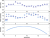 |
Fig. 1 Average atmospheric conditions during the ZIMPOL observations. The x-axis shows the average conditions in cycles of 10 min. Therefore, we have represented 19 cycles of 10 min each. From top to bottom, we have plotted the coherence time (τ0), the average FWHM as seen by the guide probe at the beginning and end of the cycles, and the airmass. |
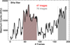 |
Fig. 2 Maximum counts (in ADU) measured in the 190 individual frames obtained in the B_Ha filter. The gray shaded areas correspond to the 76 selected images (see text), while the hatched red area corresponds to the best 47 individual exposures. |
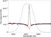 |
Fig. 3 The observed CAFE/CAHA spectrum around the Hα line (in black). The red line represents the model used to fit the stellar atmosphere (see text). The dashed blue line represents the ZIMPOL B_Ha filter transmission curve. |
2.2 CAHA/CAFE spectroscopy
To complement the SPHERE/ZIMPOL observations, we performed high-resolution spectroscopy of MWC 758 with the CAFE spectrograph attached to the 2.2 m telescope in the Calar Alto Observatory (Aceituno et al. 2013). CAFE is equipped with a 2.′′ 4 diameter optical fibre, and provides high-resolution spectra (R ~ 63 000) over the 3900–9600 Å spectral range.
We obtained a spectrum on the night of December 24, 2015 under photometric conditions and with an average seeing of 0.′′ 7. The total exposure time was 600 s. The spectrum was reduced with a dedicated pipeline developed by the observatory and explained in Aceituno et al. (2013). The processing was as follows: the data were bias subtracted and flat-field corrected. We used thorium-argon (ThAr) exposures obtained after the science spectrum to wavelength-calibrate the data. The spectrum was flux-calibrated using the standard star HD 19445, observed one hour before the science target with an airmass difference of ~0.2. We compared the calibrated spectrum with published photometry (Beskrovnaya et al. 1999), obtaining that the spectrum is ~1.2 times brighter (0.2 mag) in the R-band. Therefore, we estimate a precision in the flux calibration of ~20% in this band.
Figure 3 shows a portion of the calibrated CAFE spectrum containing the Hα line. We measure a line flux of 1.3 ± 0.3 × 10⁻¹¹ erg s−1 cm−2. To correct for the stellar photospheric absorption, we first computed synthetic spectra using the codes ATLAS and SYNTHE (Kurucz 1993) fed with the models describing the stratification of the stellar atmospheres (Castelli & Kurucz 2003). Solar abundances were assumed. The synthetic spectrum was computed assuming Teff = 7750 K and logg* = 4.0 as the starting point, following the result from Beskrovnaya et al. (1999). A value of v sin i = 50 km s−1 was adopted since it reproduces well the width of the photospheric line profiles. The model is displayed as a red line in Fig. 3. The estimated Hα line flux, corrected from the photospheric absorption, is 1.6 ± 0.3 × 10⁻¹¹ erg s−1 cm−2. Taking into account the reported visual extinction of AV = 0.16 mag (Meeus et al. 2012), we can correct the flux adopting a value of AR ~ 0.12 mag (Rieke & Lebofsky 1985), and estimate a line luminosity of ~0.013 L⊙ for a distance of 151 pc.
Assuming that the Herbig Be/Ae relationship between Hα luminosity and accretion luminosity derived by Fairlamb et al. (2017) holds, we estimate  . We derive Lacc = 1.6 ± 0.4 L⊙. Following Mendigutía et al. (2011), we estimate a mass accretion rate of ~ (7± 2) × 10−8 M⊙ yr−1, for a stellar mass of 1.4±0.3 M⊙ and a stellarradius of 2 R⊙ (Boehler et al. 2018), already scaled to the Gaia distance.
Finally, we note that although the CAFE spectrum is not simultaneous to the SPHERE observations, it allows us to characterize the primary star and to double-check the calibration of our ZIMPOL data with close in-time observations.
3 Results and discussion
The SPHERE/ZIMPOL combined images of MWC 758 in the B_Ha and the Cnt_Ha filters, together with the differential B_Ha–Cnt_Ha image, are displayed in Fig. 4. We show the results of combining the 47 best images. We have not detected any point-like source in any of the analyzed datasets. The 5σ contrast achieved in the two individual filters, and in the differential sequence, is displayed in Fig. 5. We reach ~7.6 mag in the B_Ha and the Cnt_Ha filters at a separation of 111 mas, that is, where the protoplanet candidate by Reggiani et al. (2018) is detected.
The fact that we do not detect any companion in the individual filters and differential images does not allow us a direct estimation of its Hα flux. However, since the 47 images were observed under photometric conditions, we can convert the B_Ha contrast curve into fluxes by calibrating the counts (cts) from the primary star. To this aim, we first performed aperture photometry of the central star in ten individual images (out of the 47), using a large aperture radius (320 pixel radius, ~1 arcsec). We obtain a total of ~6.5(±0.6) × 106 cts. The uncertainty includes a relative error of 10% associated to the channel splitting, and the background error estimation. We converted the integrated counts into fluxes using the zero-points (ZPs) derived by Schmid et al. (2017), and their Eq. (4):
 (1)
(1)
Assuming that all the emission in the B_Ha filter comes from the Hα line, we can convert the counts per second adopting a zero-point ( ) of 7.2(±0.4)×10−16 erg/(cm2 ct), and an mmode value of −0.23 mag to take into account the usage of the R-band dichroic (Schmid, private communication). For an average airmass (am) of 1.57 (for the 47 images), and a typical R-band atmospheric extinction value of k1 ~ 0.08 (Patat et al. 2011), we obtained a B_Ha flux of ~ 7.1(±0.8) × 10−11 erg s−1 cm−2 for the primary star. We note that the assumption that all the counts in the B_Ha filter come from the line results in a line flux overestimation of a factor of ~5 when compared with the line flux measured directly in the spectrum.
We used the total calibrated flux in B_Ha, together with the contrast curve to derive an upper limit (5σ) to the B_Ha flux at different separations form the central object. In particular, we estimated a flux < 6.2 × 10⁻¹⁴ erg s−1 cm−2 at 111 mas, the separation of the planet candidate. If we assume that all the flux comes from the line, and an extinction equal to that of the primary star (AR = 0.12 mag), we estimate a line luminosity of 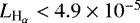 L⊙ for a distance of 151 pc. When compared with the other two Hα sources detected in transitional disks, we see that our ZIMPOL upper limit is of the same order of the emission of the protoplanet candidate LkCa15 b (6 × 10⁻⁵ L⊙, Sallum et al. 2015), and one order of magnitude fainter than the very low-mass star (~ 0.2M⊙) HD142527 B (5 × 10⁻⁴ L⊙, Close et al. 2014). We note that the smallest and lightest accreting companions to stars in the brown dwarf/planet boundary (e.g., GQ Lup b, FW Tau b, GSC 06214–0210 b, DH Tau b) show Hα luminosity values in the range
  – 6.5 × 10⁻⁷L⊙ (see e.g., Bowler et al. 2014; Zhou et al. 2014).
As explained in Reggiani et al. (2018), the mass of the companion candidate (Mp) should be below 5.5 MJup to allow for small dust replenishment within the disk. The comparison of their L′ -band luminosity with circumplanetary accretion models (Zhu 2015) is consistent with  yr−1 for disk inner radii of Rin = 1−4 RJup, respectively (see their Fig. 6). Given the mass constraints, their data is compatible with a 0.5–5 MJup protoplanet with an accretion rate of 10−7−10−9 M⊙ yr−1.
As a first approximation, and following previous works (Close et al. 2014; Sallum et al. 2015), we can estimate the accretion luminosity (Lacc) of MWC 758 b assuming that it scales with  as in classical T Tauri stars (CTTSs). In this case,
 ![Mathematical equation: $L_{\textrm{acc}} = 10^{[(2.99\pm0.16) + (1.49\pm0.05)*\log (L_{\textrm{H}_{\mathrm{\alpha}}})]}$](/articles/aa/full_html/2018/05/aa32874-18/aa32874-18-eq10.png) (Rigliaco et al. 2012), and we derive an upper limit of Lacc < 3.7 × 10⁻⁴ L⊙ at 111 mas. Using the Lacc upper limit, and following Gullbring et al. (1998), we estimate
(Rigliaco et al. 2012), and we derive an upper limit of Lacc < 3.7 × 10⁻⁴ L⊙ at 111 mas. Using the Lacc upper limit, and following Gullbring et al. (1998), we estimate  yr−1, assuming a planet radius of 1.1 RJup (the average value for 0.5-5MJup planets according to 3 Myr COND models, Baraffe et al. 2003). This upper limit is consistent with the lowest values of Mp Ṁ derived for Rin =1 RJup by Reggiani et al. (2018). If we assume planet masses of 0.5–5 MJup and a planet radius of 1.1 RJup, we estimate accretion rates of Ṁ < 3.4 × (10−8−10−9) M⊙ yr−1 for MWC 758 b.
We note, however, that low-mass brown dwarfs and planetary mass objects seem not to follow the  –Lacc relation derived for CTTSs: as an example, Zhou et al. (2014) estimated the accretion rates of three very low-mass substellar sources through their UV/optical excesses, and found values more than one order of magnitude higher than the values expected from extrapolating the CTTSs relationship. Interestingly, they also show that, in contrast with young TTSs, very low-mass accreting objects might emit a larger fraction of their accretion luminosity in the Hα line.
An alternative way to study the Hα emission of protoplanets is to compare their estimated luminosity with predictions from accreting circumplanetary models (Zhu 2015). In this latter work, the author studied the expected Hα emission from protoplanets due to magnetospheric accretion (see their Eq. (22)), obtaining upper limits to their  luminosity three orders of magnitude lower than the typical values derived for CTTSs (~ 5 × 10⁻³ L⊙, Rigliaco et al. 2012). The line luminosity depends on the truncation radius of the inner disk, and the infall velocity of the accreted material. According to their Eq. (22), our ZIMPOL data (
 ) is consistent with their predicted luminosity for truncation radii smaller than ~3.2 RJup.
The fact that we do not detect any source in the B_Ha filter might suggest that the MWC 758 protoplanet candidate is accreting at a low rate and we are not sensitive to its Hα emission. Another possibility is that the object is undergoing episodic accretion and we have observed it in a quiescent state. Although the disk inclination is closer to face-on, the sub-millimetercavity is filled with small grains (Benisty et al. 2015), so the object might also be too extincted and therefore undetectable in the optical regime. Finally, we cannot exclude the possibility that the L′ infrared emission is related to a disk asymmetry and not with a protoplanet, as proposed by Reggiani et al. (2018). In fact, it is known that ADI techniques can highlight disk features in such a way that they can look like planets, especially for low-inclination systems (see e.g., Ligi et al. 2018). Follow-up L′ observations, together with deeper K-band data, will help to understand the true nature of the infrared detection.
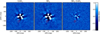 |
Fig. 4 VLT/ZIMPOL ADI reduced images of MWC 758 processed with PCA (5 modes) in the Cnt_Ha (left) and B_Ha (center) filters. The ASDI image (B_Ha-Cnt_Ha) processed with PCA (5 modes) is displayed in the right panel. North is up and East to the left. The red circle shows the position at a separation of 111 mas, and a PA of 165.5°, where the companion candidate was detected by Reggiani et al. (2018) in the L′ -band. |
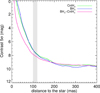 |
Fig. 5 VLT/ZIMPOL 5σ contrast curves obtained in Cnt_Ha and B_Ha in ADI using PCA, and in B_Ha-Cnt_Ha in ASDI using PCA. The gray area shows the position of the companion candidate detected at L′ by Reggiani et al. (2018). The curves are derived using the best 47 images. |
Acknowledgements
We are grateful to the referee, C. Grady, whose comments helped to improve this manuscript. This research has been funded by Spanish grants ESP2015-65712-C5-1-R and ESP2017-87676-C5-1-R. NH is indebted to the Paranal staff that gave their support during the observations, and to the CAHA staff. Part of this work has been carried out within the framework of the National Centre for Competence in Research PlanetS supported by the Swiss National Science Foundation. S.P.Q. and H.M.S. acknowledge the financial support of the SNSF. JMA acknowledge financial support from the project PRIN-INAF 2016 The Cradle of Life – GENESIS-SKA (General Conditions in Early Planetary Systems for the rise of life with SKA). I.M. acknowledges the financial support of the Government of Comunidad Autónoma de Madrid (Spain) through a “Talento” Fellowship (2016-T1/TIC-1890). Based on observations collected at the Centro Astronómico Hispano Alemán (CAHA) at Calar Alto, operated jointly by the Max-Planck Institut für Astronomie and the Instituto de Astrofísica de Andalucía (CSIC). This work has made use of data from the European Space Agency (ESA) mission Gaia (https://www.cosmos.esa.int/gaia), processed by the Gaia Data Processing and Analysis Consortium (DPAC, https://www.cosmos.esa.int/web/gaia/dpac/consortium). Funding for the DPAC has been provided by national institutions, in particular the institutions participating in the Gaia Multilateral Agreement.
References
- Aceituno, J., Sánchez, S. F., Grupp, F., et al. 2013, A&A, 552, A31 [NASA ADS] [CrossRef] [EDP Sciences] [Google Scholar]
- Andrews, S. M., Wilner, D. J., Espaillat, C., et al. 2011, ApJ, 732, 42 [NASA ADS] [CrossRef] [Google Scholar]
- Baraffe, I., Chabrier, G., Barman, T. S., Allard, F., & Hauschildt, P. H. 2003, A&A, 402, 701 [NASA ADS] [CrossRef] [EDP Sciences] [Google Scholar]
- Benisty, M., Juhasz, A., Boccaletti, A., et al. 2015, A&A, 578, L6 [NASA ADS] [CrossRef] [EDP Sciences] [Google Scholar]
- Beskrovnaya, N. G., Pogodin, M. A., Miroshnichenko, A. S., et al. 1999, A&A, 343, 163 [NASA ADS] [Google Scholar]
- Beuzit, J.-L., Feldt, M., Dohlen, K., et al. 2008, Ground-based and Airborne Instrumentation for Astronomy II, in Proc. SPIE, 7014 701418 [CrossRef] [Google Scholar]
- Biller, B. A., Males, J., Rodigas, T., et al. 2014, ApJ, 792, L22 [NASA ADS] [CrossRef] [Google Scholar]
- Boccaletti, A., Pantin, E., Lagrange, A.-M., et al. 2013, A&A, 560, A20 [NASA ADS] [CrossRef] [EDP Sciences] [Google Scholar]
- Boehler, Y., Ricci, L., Weaver, E., et al. 2018, ApJ, 853, 162 [Google Scholar]
- Bowler, B. P., Liu, M. C., Kraus, A. L., & Mann, A. W. 2014, ApJ, 784, 65 [NASA ADS] [CrossRef] [Google Scholar]
- Castelli, F. & Kurucz, R. L. 2003, in Modelling of Stellar Atmospheres, eds. N. Piskunov, W. W. Weiss, & D. F. Gray, IAU Symp., 210, A20 [Google Scholar]
- Chapillon, E., Guilloteau, S., Dutrey, A., & Piétu, V. 2008, A&A, 488, 565 [NASA ADS] [CrossRef] [EDP Sciences] [Google Scholar]
- Chauvin, G., Lagrange, A.-M., Beust, H., et al. 2012, A&A, 542, A41 [NASA ADS] [CrossRef] [EDP Sciences] [Google Scholar]
- Close, L. M., Follette, K. B., Males, J. R., et al. 2014, ApJ, 781, L30 [NASA ADS] [CrossRef] [Google Scholar]
- Dong, R., Zhu, Z., Rafikov, R. R., & Stone, J. M. 2015, ApJ, 809, L5 [NASA ADS] [CrossRef] [Google Scholar]
- Fairlamb, J. R., Oudmaijer, R. D., Mendigutia, I., Ilee, J. D., & van den Ancker, M. E. 2017, MNRAS, 464, 4721 [NASA ADS] [CrossRef] [Google Scholar]
- Gaia Collaboration (Brown, A. G. A., et al.) 2016a, A&A, 595, A2 [NASA ADS] [CrossRef] [EDP Sciences] [Google Scholar]
- Gaia Collaboration (Prusti, T., et al.) 2016b, A&A, 595, A1 [NASA ADS] [CrossRef] [EDP Sciences] [Google Scholar]
- Grady, C. A., Muto, T., Hashimoto, J., et al. 2013, ApJ, 762, 48 [NASA ADS] [CrossRef] [Google Scholar]
- Gullbring, E., Hartmann, L., Briceño, C., & Calvet, N. 1998, ApJ, 492, 323 [NASA ADS] [CrossRef] [Google Scholar]
- Huélamo, N., Lacour, S., Tuthill, P., et al. 2011, A&A, 528, L7 [NASA ADS] [CrossRef] [EDP Sciences] [Google Scholar]
- Isella, A., Natta, A., Wilner, D., Carpenter, J. M., & Testi, L. 2010, ApJ, 725, 1735 [NASA ADS] [CrossRef] [Google Scholar]
- Kraus, A. L., & Ireland, M. J. 2012, ApJ, 745, 5 [NASA ADS] [CrossRef] [Google Scholar]
- Kurucz, R. 1993, SYNTHE Spectrum Synthesis Programs and Line Data. Kurucz CD-ROM No. 18 (Cambridge, MA: Smithsonian Astrophysical Observatory), 18 [Google Scholar]
- Lafrenière, D., Marois, C., Doyon, R., Nadeau, D., & Artigau, É. 2007, ApJ, 660, 770 [NASA ADS] [CrossRef] [Google Scholar]
- Ligi, R., Vigan, A., Gratton, R., et al. 2018, MNRAS, 473, 1774 [NASA ADS] [CrossRef] [Google Scholar]
- Marino, S., Casassus, S., Perez, S., et al. 2015, ApJ, 813, 76 [NASA ADS] [CrossRef] [Google Scholar]
- Marois, C., Lafrenière, D., Doyon, R., Macintosh, B., & Nadeau, D. 2006, ApJ, 641, 556 [Google Scholar]
- Mawet, D., Milli, J., Wahhaj, Z., et al. 2014, ApJ, 792, 97 [NASA ADS] [CrossRef] [Google Scholar]
- Mayama, S., Hashimoto, J., Muto, T., et al. 2012, ApJ, 760, L26 [NASA ADS] [CrossRef] [Google Scholar]
- Meeus, G., Montesinos, B., Mendigutía, I., et al. 2012, A&A, 544, A78 [NASA ADS] [CrossRef] [EDP Sciences] [Google Scholar]
- Mendigutía, I., Calvet, N., Montesinos, B., et al. 2011, A&A, 535, A99 [NASA ADS] [CrossRef] [EDP Sciences] [Google Scholar]
- Mendigutía, I., Oudmaijer, R. D., Garufi, A., et al. 2017, A&A, 608, A104 [NASA ADS] [CrossRef] [EDP Sciences] [Google Scholar]
- Patat, F., Moehler, S., O’Brien, K., et al. 2011, A&A, 527, A91 [NASA ADS] [CrossRef] [EDP Sciences] [Google Scholar]
- Pérez, L. M., Carpenter, J. M., Andrews, S. M., et al. 2016, Science, 353, 1519 [NASA ADS] [CrossRef] [Google Scholar]
- Pinilla, P., de Boer, J., Benisty, M., et al. 2015, A&A, 584, L4 [NASA ADS] [CrossRef] [EDP Sciences] [Google Scholar]
- Pohl, A., Benisty, M., Pinilla, P., et al. 2017, ApJ, 850, 52 [NASA ADS] [CrossRef] [Google Scholar]
- Quanz, S. P., Amara, A., Meyer, M. R., et al. 2013, ApJ, 766, L1 [NASA ADS] [CrossRef] [Google Scholar]
- Racine, R., Walker, G. A. H., Nadeau, D., Doyon, R., & Marois, C. 1999, PASP, 111, 587 [NASA ADS] [CrossRef] [Google Scholar]
- Reggiani, M., Christiaens, V., Absil, O., et al. 2018, A&A, 611, A74 [NASA ADS] [CrossRef] [EDP Sciences] [Google Scholar]
- Rieke, G. H., & Lebofsky, M. J. 1985, ApJ, 288, 618 [NASA ADS] [CrossRef] [Google Scholar]
- Rigliaco, E., Natta, A., Testi, L., et al. 2012, A&A, 548, A56 [NASA ADS] [CrossRef] [EDP Sciences] [Google Scholar]
- Sallum, S., Follette, K. B., Eisner, J. A., et al. 2015, Nature, 527, 342 [NASA ADS] [CrossRef] [Google Scholar]
- Schmid, H. M., Bazzon, A., Milli, J., et al. 2017, A&A, 602, A53 [NASA ADS] [CrossRef] [EDP Sciences] [Google Scholar]
- Soummer, R., Pueyo, L., & Larkin, J. 2012, ApJ, 755, L28 [NASA ADS] [CrossRef] [Google Scholar]
- Thalmann, C., Schmid, H. M., Boccaletti, A., et al. 2008, Ground-based and Airborne Instrumentation for Astronomy II, in Proc. SPIE, 7014, 70143F [Google Scholar]
- van Leeuwen, F. 2007, A&A, 474, 653 [NASA ADS] [CrossRef] [EDP Sciences] [Google Scholar]
- Whelan, E. T., Huélamo, N., Alcalá, J. M., et al. 2015, A&A, 579, A48 [NASA ADS] [CrossRef] [EDP Sciences] [Google Scholar]
- Zhou, Y., Herczeg, G. J., Kraus, A. L., Metchev, S., & Cruz, K. L. 2014, ApJ, 783, L17 [NASA ADS] [CrossRef] [Google Scholar]
- Zhu, Z. 2015, ApJ, 799, 16 [NASA ADS] [CrossRef] [Google Scholar]
All Figures
|
Fig. 1 Average atmospheric conditions during the ZIMPOL observations. The x-axis shows the average conditions in cycles of 10 min. Therefore, we have represented 19 cycles of 10 min each. From top to bottom, we have plotted the coherence time (τ0), the average FWHM as seen by the guide probe at the beginning and end of the cycles, and the airmass. |
| In the text | |
|
Fig. 2 Maximum counts (in ADU) measured in the 190 individual frames obtained in the B_Ha filter. The gray shaded areas correspond to the 76 selected images (see text), while the hatched red area corresponds to the best 47 individual exposures. |
| In the text | |
|
Fig. 3 The observed CAFE/CAHA spectrum around the Hα line (in black). The red line represents the model used to fit the stellar atmosphere (see text). The dashed blue line represents the ZIMPOL B_Ha filter transmission curve. |
| In the text | |
|
Fig. 4 VLT/ZIMPOL ADI reduced images of MWC 758 processed with PCA (5 modes) in the Cnt_Ha (left) and B_Ha (center) filters. The ASDI image (B_Ha-Cnt_Ha) processed with PCA (5 modes) is displayed in the right panel. North is up and East to the left. The red circle shows the position at a separation of 111 mas, and a PA of 165.5°, where the companion candidate was detected by Reggiani et al. (2018) in the L′ -band. |
| In the text | |
|
Fig. 5 VLT/ZIMPOL 5σ contrast curves obtained in Cnt_Ha and B_Ha in ADI using PCA, and in B_Ha-Cnt_Ha in ASDI using PCA. The gray area shows the position of the companion candidate detected at L′ by Reggiani et al. (2018). The curves are derived using the best 47 images. |
| In the text | |
Current usage metrics show cumulative count of Article Views (full-text article views including HTML views, PDF and ePub downloads, according to the available data) and Abstracts Views on Vision4Press platform.
Data correspond to usage on the plateform after 2015. The current usage metrics is available 48-96 hours after online publication and is updated daily on week days.
Initial download of the metrics may take a while.