| Issue |
A&A
Volume 613, May 2018
|
|
|---|---|---|
| Article Number | A49 | |
| Number of page(s) | 12 | |
| Section | Interstellar and circumstellar matter | |
| DOI | https://doi.org/10.1051/0004-6361/201732296 | |
| Published online | 30 May 2018 | |
Widespread HCN maser emission in carbon-rich evolved stars★
1
Max-Planck-Institut für Radioastronomie,
Auf dem Hügel 69,
53121
Bonn,
Germany
e-mail: kmenten@mpifr.de
2
Instituut voor Sterrenkunde, Katholieke Universiteit Leuven,
Celestijnenlaan 200D,
3001
Leuven,
Belgium
3
Harvard-Smithsonian Center for Astrophysics,
60 Garden Street,
Cambridge,
MA
02138,
USA
Received:
14
November
2017
Accepted:
9
January
2018
Context. HCN is a major constituent of the circumstellar envelopes of carbon-rich evolved stars, and rotational lines from within its vibrationally excited states probe parts of these regions closest to the stellar surface. A number of such lines are known to show maser action. Historically, in one of them, the 177 GHz J = 2 → 1 line in the l-doubled bending mode has been found to show relatively strong maser action, with results only published for a single object, the archetypical high-mass loss asymptotic giant branch (AGB) star IRC+10216.
Aims. To examine how common 177 GHz HCN maser emission is, we conducted an exploratory survey for this line toward a select sample of carbon-rich asymptotic giant branch stars that are observable from the southern hemisphere.
Methods. We used the Atacama Pathfinder Experiment 12 meter submillimeter Telescope (APEX) equipped with a new receiver to simultaneously observe three J = 2 → 1 HCN rotational transitions, the (0, 11c, 0) and (0, 11d, 0) l-doublet components, and the line from the (0,0,0) ground state.
Results. The (0, 11c, 0) maser line is detected toward 11 of 13 observed sources, which all show emission in the (0,0,0) transition. In most of the sources, the peak intensity of the (0, 11c, 0) line rivals that of the (0,0,0) line; in two sources, it is even stronger. Except for the object with the highest mass-loss rate, IRC+10216, the (0, 11c, 0) line covers a smaller velocity range than the (0,0,0) line. The (0, 11d, 0) line, which is detected in four of the sources, is much weaker than the other two lines and covers a velocity range that is smaller yet, again except for IRC+10216. Compared to its first detection in 1989, the profile of the (0, 11c, 0) line observed toward IRC+10216 looks very different, and we also appear to see variability in the (0,0,0) line profile (at a much lower degree). Our limited information on temporal variabilitydisfavors a strong correlation of maser and stellar continuum flux.
Conclusions. Maser emission in the 177 GHz J = 2 → 1 (0, 11c, 0) line of HCN appears to be common in carbon-rich AGB stars. Like for other vibrationally excited HCN lines, our observations indicate that the origin of these lines is in the acceleration zone of the stellar outflow in which dust is forming. For all the stars toward which we detect the maser line, the number of photons available at 7 and 14 μm, corresponding to transitions to vibrationally excited states possibly involved in its pumping, is found to be far greater than that of the maser photons, which makes radiative pumping feasible. Other findings point to a collisional pumping scheme, however.
Key words: masers / stars: AGB and post-AGB / stars: carbon / circumstellar matter
The reduced spectra (FITS files) are only available at the CDS via anonymous ftp to cdsarc.u-strasbg.fr (130.79.128.5) or via http://cdsarc.u-strasbg.fr/viz-bin/qcat?J/A+A/613/A49
© ESO 2018
1 Introduction: HCN in carbon-rich evolved stars and elsewhere
Hydrogen cyanide (HCN), one of the first molecules discovered by millimeter-wavelength astronomy (Snyder & Buhl 1971), is a common molecular species in the interstellar medium (ISM), namely in star-forming regions. Moreover, HCN is also abundant in the atmospheres and the circumstellar envelopes (CSEs) of carbon-rich asymptotic giant branch (AGB) stars. The substantial electric dipole moment of the HCN molecule, 2.99 D (Ebenstein & Muenter 1984), makes its pure rotational lines probes of the denser ISM and CSE environments.
In the atmospheres of cool C-rich AGB stars (“C-Miras”), stars whose abundance of carbon is higher than that of oxygen, after H2 and CO, HCN becomes the third most abundant “parent” molecule (Tsuji 1964; Cherchneff 2006); Schöier et al. (2013) derived a median HCN/H2 abundance ratio of 3∕105 for a sample of C-rich AGB stars. Since the detection of its J = 1 → 0 ground-state line toward the archetypical high mass-loss very evolved C-rich AGB star IRC+10216 (CW Leo, Morris et al. 1971), rotational lines from levels with higher angular momentum quantum number, J, from the vibrational ground state have been detected, as well as a wide variety of rotational lines from excited vibrational states, starting with the study of Ziurys & Turner (1986). Most of these lines were found in the nearby IRC+10216 (e.g., Avery et al. 1994; Groesbeck et al. 1994; Cernicharo et al. 2011), but vibrationally excited HCN emission was also detected toward other C-rich AGB stars (e.g., Bieging 2001), the more evolved protoplanetary nebula CRL 618 (Thorwirth et al. 2003b), in star-forming regions (e.g., Ziurys & Turner 1986; Rolffs et al. 2011; Veach et al. 2013), and even in the warm and dense core regions of starburst galaxies (Salter et al. 2008; Sakamoto et al. 2010).
Strong maser amplification from molecules around C-rich evolved stars is much rarer than for O-rich stars, which very frequently host maser emission in a plethora of transitions from the SiO and H2 O molecules (see, e.g., Gray 2012; Gray et al. 2016). Vibrationally excited HCN lines account for most of the known masing transitions found so far toward C-rich stars. The two most prominent of these consist of low J lines from within the two lowest vibrationally excited states of the l-doubled bending mode with energies of ≈1030 and 2060 K above the ground state (Guilloteau et al. 1987; Lucas et al. 1988; Lucas & Cernicharo 1989). Bieging (2001) gives a summary of stellar HCN masers and also reports the first detection of maser emission in the J = 3 → 2 and 4 → 3 transitions of the (0, 1 1c, 0) state. All the stars hosting such masers appear to have relatively high mass-loss rates on the order of 10−6 to 10−5 M⊙ yr−1. From much more highly excited states, laser emission was detected in the J = 9 − 8 rotational line from the third overtone of a bendingmode state, (0, 40, 0), and also in the J = 10 − 9 lines between the Coriolis-coupled (1, 11, 1) and (0, 40, 0) states (Schilke et al. 2000; Schilke & Menten 2003). These lines have upper-level energies around 4200 K. At the other extreme, evidence for maser emission has been reported in the lowest frequency (J = 1 → 0) rotational line of the vibrational ground state toward optically bright “blue” carbon stars (Izumiura et al. 1995; Olofsson et al. 1998) that have much lower mass-loss rates than the values quoted above.
A relatively strong (~400 Jy) HCN maser line connecting the J = 2 and 1 rotational levels within the (0, 11c, 0) (≡ v2 = 1c) l-doubled vibrationally excited bending mode state of HCN1 was discovered toward IRC+10216 by Lucas & Cernicharo (1989). Given its elevated lower level energy (1029 K), it is clear that this line arises from the inner regions of the CSE of this object. In a Note added in proof to the Letter reporting their discovery, Lucas & Cernicharo (1989) mention that “a preliminary search in similar objects has led to six detections”.
In 2015, the new SEPIA receiver was commissioned on the Atacama Pathfinder Experiment 12 meter telescope, APEX2. It covers the 157–212 GHz range and thus, near 177 GHz, the frequencies of three HCN J = 2 → 1 rotational lines, namely the (0, 11c, 0) maser transition, its from the vibrational ground state. All three can be observed simultaneously.
Here we report on an exploratory survey for these three lines toward a sample of (mostly) southern C-rich AGB stars. In Sect. 2 we introduce our observed sample. In Sect. 3 we describe the observations made with the APEX telescope and present the data we obtained. This is followed by a brief general description of HCN spectroscopy relevant to our study (Sect. 4). Our results are presented in Sect. 5 and discussed in Sect. 6, where special emphasis is given to IRC+10216. We summarize our results and present an outlook on future studies in Sect.7.
2 Sample of C-rich carbon stars
Our sample is presented in Table 1. For this first APEX survey, we made a “success-oriented” selection of C-rich AGB stars that are known to have HCN emission in the vibrational ground-state J = 1 → 0 line as listed in the catalog of Loup et al. (1993). For most sources we present two estimates for their distance: the first, DBF, comes from Loup et al. (1993), who compiled or estimated bolometric fluxes for a sample of AGB stars and assumed, uniformly, a luminosity of 104 L⊙. The second, DPLR, was obtained from the catalog published by Menzies et al. (2006). These values were obtained using the well-defined C-Mira period-luminosity relation established by Feast et al. (1989) and Whitelock et al. (2003) and are mostly based on a new dataset presented by Whitelock et al. (2006). For some stars, period and phase were derived from visual data available through the web site of AAVSO’s International Variable Star Index3. Details on the phase determinations are given in Appendix A. When both distances are available, they agree quite well for most of the objects, that is, theyagree to within 30%. Because of the rather simplistic assumption of a uniform luminosity made by Loup et al., in this paper DPLR is used for the distance when available. If it is not, we use DBF. Published values of the stellarLSR velocities,  , and the terminal velocities of their CSEs,
  , were again taken from the Loup et al. (1993) catalog or from Olofsson et al. (1993). In both papers these values were determined from spectra of the CO J = 1 → 0 and 2 → 1 lines (and also from HCN J = 1 → 0 spectra in the former). For the stellar mass-loss rates, Ṁ, we present a range of values that envelop the numbers given by Loup et al. (1993) and Olofsson et al. (1993). These values are based on modeling of CO line data. A discussion of the large spread in Ṁ is beyond the scope this paper, in which mass-loss rate is only invoked in a qualitative discussion of the propensity to find maser emission as a function of this quantity.
3 Observations
Our observations were made on 2015 May 28 under excellent weather conditions with the 12 m diameter APEX submillimeter telescope (Güsten et al. 2006)under project number M-095.F-9544A-2015. The amount of precipitable water vapor in the atmosphere as monitored by the APEX radiometer4 was 0.9 mmin the atmosphere above the Llano de Chajnantor.
We used the new prototype receiver developed for frequency band 5 of the Atacama Large Millimeter/submillimeter Array (ALMA). At the APEX telescope, it is a component of SEPIA, the Swedish-ESO PI receiver for APEX (Billade et al. 2012; Immer et al. 2016). This is a dual-polarization sideband-separated (2SB) receiver that covers the frequency range 157.36–211.64 GHz. In particular, the central part of this band has been relatively little explored in the past because of strong atmospheric absorption caused by the 313 − 220 line of para-H2O near 183 GHz. At the excellent site at 5100 m at which ALMA and APEX are located, the transmission in this band is quite acceptable for most of the time, and maser emission in this very H2 O line has previously been observed with APEX toward a variety of astronomical sources (Immer et al. 2016; Humphreys et al. 2017).
Each sideband of the receiver has a total bandwidth of 4 GHz. The central frequencies of the two sidebands are separated by 12 GHz, corresponding to an intermediate frequency (IF) band of 4–8 GHz. We centered the signal IF band at 177.780 GHz, a frequency close to our main target lines listed in Table 2. For our observations we wobbled the telescope subreflector with a rate of 1.5 Hz between positions that were symmetrically offset in azimuth by 60″, larger than any plausible HCN emission distribution (see Sect. 6.1.1). Total observing times ranged from (mostly) ~0.5 h up to 2 h for the weaker sources. Calibration was obtained using the chopper-wheel technique under consideration of the different atmospheric opacities in the signal and image sidebands of the employed 2SB receiver. The radiation was analyzed with the newest implementation of the MPIfR-built fast Fourier transform spectrometer (Klein et al. 2006), which accounted for redundant overlap between sub modules and provided 52 430 frequency channels over the 4 GHz wide intermediate frequency bandwidth with a channel spacing of 76.3 kHz, corresponding to 0.13 km s−1. To increase the signal-to-noise ratio (S/N) the spectra were smoothed to effective velocity resolutions appropriate for the measured widths even of narrow features, that is, ~0.5–1 km s−1.
To check the telescope pointing, we used either the signal from the HCN J =2 → 1 lines from the program stars themselves or that from the SiO v = 1, J = 4 → 3 maser line (172 481.1175 MHz) from an O-rich AGB star close in the sky to one of our C-rich program stars. Five-point crosses centered on the stellar position with half-beam width offsetsin elevation and azimuth were measured. Pointing corrections were derived from these measurements. The pointing was found to be accurate to within ≈ 3″, acceptable given the full-width at half-maximum (FWHM) beam size, θB, which is 36″ at 177 GHz. We established a main-beam brightness temperature, TMB, scale (in K) by extrapolating the main-beam efficiencies, ηMB, from higher-frequency values observationally, determined by Güsten et al. (2006), to 177 GHz. We assumed ηMB = 0.7. This value was validated by observations of Uranus. Our TMB values can be multiplied by a factor of 33.4 to convert them into flux density units (in Jy).
Stellar sample information.
4 HCN vibration-rotational spectroscopy
4.1 HCN vibrational modes
The HCN molecule has three fundamental vibrational states: the CH stretching mode, designated ν1 [or (1,0,0)], the doubly degenerate bending mode, ν2 [or (0,1,0)], and the CN stretching mode, ν3 [or (0,0,1)]. The wavelengths of the fundamental transitions of these modes are 3.0, 14.0, and 4.9 μm, and they correspond to temperatures of 2931, 1025, and 4841 K (Adel & Barker 1934). Because of the Earth’s atmosphere, direct ro-vibrational lines cannot easily be observed from the ground. Cernicharo et al. (1999) used the Short Wavelength Spectrometer (SWS) on board the Infrared Space Observatory (ISO) to study such lines from the stretching and the bending modes, including overtone and combinations bands toward IRC+10216.
Each vibrational state contains a ladder of rotational levels, characterized by the angular momentum quantum number J. Rotational (J → J − 1) transitions can be observed from the ground for many J between 1 and 12. Compared to the IR bands mentioned above, these lines can be studied with very high spectral resolution (>105), and their emission can also be imaged with sub-arcsecond angular resolution and superb sensitivity with interferometers such as the IRAM NOrthern Extended Millimeter Array (NOEMA) and ALMA.
4.2 l-type doubling of the ν2 bending-mode levels
Since H–C–N can bend in two orthogonal directions, the ν2 vibrationally excited bending mode is doubly degenerate. When the molecule is rotating and bending simultaneously, that is, J >0, this degeneracy is lifted, resulting in l-type doubling with every rotational level being split into two sub-levels (Nielsen 1950). The separation between these sub-levels increases with J and is given by
 (1)
(1)
where in the ν2 = 1 state, Δ νJ=1 = 448.9430 MHz (in frequency units) for the J = 1 level; see Maki & Lide (1967) and updated values listed in the Cologne Database for Molecular Spectroscopy, CDMS (Müller et al. 2005)5. The line connecting the lower (0, 11c, 0) components of the ν2 = 1 doublet has an ≈ J × 11 MHz lower frequency than the (0,0,0) line with the same J, while the (0, 11d, 0) line, which connects the upper levels, has a frequency that is higher than that of the latter line by the amount given by the difference of Eq. (1) evaluated, in our case, for J = 2 and J = 1. Note that several studies use a different nomenclature for the vibrationally excited l-doublet states: 11e and 11f instead of 11c and 11d for the lower and upper sub-levels, respectively. For consistency with previous work on the (0, 1 1c, 0) line, we here adhere to the latter convention.
This means that the two lowest rotational transitions in the ν2 = 1 vibrationally excited state, the J = 2 → 1 lines, are separated by 897.8222 MHz and can thus be observed simultaneously and together with the (0,0,0) line within the broad bandwidth provided by the APEX FFTS; see Sect. 3. The rest frequencies of these three lines and their lower rotational level energies were taken from the CDMS and are given in Table 2.
All three lines discussed here display hyperfine structure (hfs); each is split into six components. Frequencies and other information on the hfs components can also be obtained from the CDMS (from links on the explanatory web pages for the HCN entries). The relative intensities of the components and their offsets in velocity (relative to the values calculated from the “centroid” frequencies given in Table 2) are displayed for the case of IRC+10216 in Fig. 3. They are relevant for our discussion of the line widths of individual maser features in Sect. 6.3.3.
HCN J = 2 → 1 rotational lines observed with SEPIA.
5 Results
Figures 1 and 2 present all our observed spectra that show significant HCN emission. In Table 3 we list for all three observed HCN J =2 → 1 lines the full-width at zero power (FWZP) velocity range over which significant emission is detected, our measured velocity-integrated main-beam brightness temperatures (the line fluxes), or upper limits for this quantity. We also list the ratio, R, of the (0,0,0) line flux to that of the vibrationally excited lines (or its lower limit).
The HCN (0,0,0) line is detected in all of the 13 objects that we observed. We find generally good agreement between the total velocity ranges, that is, twice the terminal velocity ( ), that we measure for this line and values found in the literature, which are mostly based on CO J =1 → 0 and 2 →1 line data (see Sect. 2). This shows that the emission of the HCN (0,0,0) J =2 → 1 line is distributed over a volume of the CSE at which its outflow has reached terminal velocity.
In some cases, the profile of the (0,0,0) line has the shape expected from an angularly unresolved very optically thick line from an expanding CSE, a parabola with marked self-absorption of its low-velocity wing (see, e.g., Olofsson et al. 1982; Morris et al. 1985). This self-absorption is also responsible for some of the differences between the values our data suggest for  and/or
  and published values. For example, for IRC+10216 (CW Leo), a somewhat higher value than our − 26.5 km s−1 is frequentlygiven for the stellar velocity. Similarly, the literature velocity values might be biased for other stars, such as II Lup, RW LMi (CIT 6) and RAFGL 4211. For CIT 6, the
  and
and  values we extracted from the (0,0,0) line show the greatest difference with published numbers. For this star and RAFGL 4211, our spectra led to an upward revision of
  compared toliterature values. We note in particular that published spectra taken with a modest S/N can be affected by the bias described above.
The (0, 11c, 0) maser line is detected in 11 sources. Toward some of them, its flux rivals that of the (0,0,0) line. In contrast, emission in the (0, 1 1d, 0) line is only found toward four of the sources with (0, 11c, 0) emission and is always much weaker.
We do not see a propensity for a detection of the maser line in sources with higher mass-loss rates or a clear relation between R and the mass-loss rates of the objects, but we note that the maser line remains undetected toward X Cnc and U Hya and is barely detected toward X Tra, three sources with the lowest mass-loss rates in our sample.
In all cases, the (0, 11c, 0) maser line profiles are asymmetric. In several objects this line shows a single narrow feature within a few km s−1 of the stellar velocity that is superposed on broader emission. Except for the cases of CW Leo and V Hya, which we discuss separately (in Sects. 6.1.1 and 6.2), the (0, 1 1c, 0) line covers asignificantly narrower velocity range than the (0,0,0) line and in AI Vol, CQ Pyx, and RW LMi the (0, 1 1d, 0) line covers an even narrower range. For most sources the bulk of emission in the (0, 1 1c, 0) maser line isblueshifted relative to the stellar velocity. The possible significance of this is discussed in Sect. 6.3.4.
6 Discussion
The vibrationally excited lines cover a narrower velocity range than the line from the vibrational ground state. The reason for this most likely is that they arise from a hot region of the CSE close to the stellar surface in which dust is still forming and the outflow has not yet reached its terminal velocity. Meaningful information on this region for a C-rich AGB star is so far only available for IRC+10216 from an analysis of many HCN transitions; see Sect. 6.1.2, in which a distance of 40 stellar radii is estimated for the size of this region, or ≈ 0.′′5. Long-baseline ALMA observations will resolve this region, as they have done in the case of the O-rich (M-type) AGB star o Ceti for emission from the SiO and H2O molecules (Wong et al. 2016).
By far the most extensive information on excited HCN in the literature exists on IRC+10216, and we now concentrate on this star.
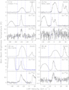 |
Fig. 1 APEX spectra of the four sources toward which all three HCN J = 2 → 1 lines are detected. For each source, the upper, middle, and lower panels show the spectra for the (0,0,0), (0, 1 1c, 0), and (0, 11d, 0) lines, respectively. 1 K TMB corresponds to a flux density of 33.4 Jy. To facilitate the comparison between the lines, we used the same intensity scale for the first two lines, except for CW Leo. In addition, for CW Leo, the TMB scale of the dotted blue line shows the base of the (0, 11c, 0) spectrum scaled up by a factor of 8 compared to the ordinate in that panel. To adequately display the weak (0, 1 1d, 0) emission, a compressed TMB scale is used for all sources for this line. The vertical dotted blue line marks the stellar velocity, while the dashed blue lines indicate the terminal velocity. The spectral line partially appearing in the (0, 1 1d, 0) spectrum of IRC+10216 at velocities > 10 km s−1 is part of a multiplet component of the N = 18 → 17 transition of C3N. |
6.1 IRC+10216
6.1.1 Variability: comparison of the IRC+10216 line profiles from two epochs
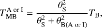
Figure 3 shows spectra of the HCN J = 2 → 1 (0,0,0) and (0, 11c, 0) lines taken 26 years apart. The top and bottom spectra were taken with the IRAM 30 m and the APEX 12 m telescopes, respectively. The IRAM spectrum was extracted from Fig. 1 of Lucas & Cernicharo (1989)6. The intensity of the (0,0,0 line) is comparable in the two spectra, 38 vs. 31 K. Since the emission from this line arises from an extended region of the CSE with a size of thousands of au (or stellar radii) and is determined by thermal processes (see below), we expect little variability of its profile. We can estimate the size of the emission region: assuming a Gaussian telescope beam with an FWHM size θB (A or I) for both the APEX and the IRAM telescopes (superscripts A and I) and a (simplifying) Gaussian source size of the HCN J = 2 → 1 (0,0,0) line emission region with an FWHM size θS, the observed main-beam brightness temperature is given by
 (2)
(2)
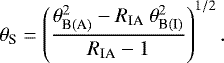
where θB(A) = 36″ and θB(I) = 15″. TB is the brightness temperatureof the emission region. Dividing this expression for the IRAM 30 m telescope by that for the APEX telescope, we can solve for the source size θS, which is given by
 (3)
(3)
Here RIA is the ratio of the main-beam brightness temperatures measured in the IRAM to that in the APEX beam, that is, 36 K/31 K = 1.16. Plugging in numbers, Eq. (3) gives a size of 80″ for the region from which the emission of the HCN J =2 → 1 (0,0,0) line arises and a strict lower limit of 48″ when we assume an uncertainty in the TB scale of 10%. The nominal value of 80″ is higher than expected, given that the emission region of the lower-critical density HCN J = 1 → 0 line has been measured to have an extent of 64″ by Dayal & Bieging (1995) with the Berkeley-Illinois-Maryland Array (BIMA). Given the calibration uncertainties in typical datasets obtained with (sub)millimeter single-dish telescopes, it is impossible to obtain a reliable estimate of the size of the J = 2 → 1 (0,0,0) line emission region without mapping. Regardless of the uncertainties in the absolute intensity calibration, when we inspect the spectrum of the (0,0,0) line closely (Fig. 3), we find other possible evidence for variability, namely the “shoulder” in its shape near an LSR velocity of − 12 km s−1, which is observed in the spectrum taken with the IRAM telescope, but not in the APEX spectrum. Variability of non-maser spectral lines might be expected and has been observed in high-excitation lines arising in the innermost CSE of IRC+10216 (Cernicharo et al. 2014; He et al. 2017). However, variability has recently also been reported for lines from some molecules whose emission arises in the outer envelope of the star, while lines from others, for example, from SiC2, remain constant (Cernicharo et al. 2014; He et al. 2017). Even the very large scale continuum emission from dust has been found to show variability, which is explained as a reflex to the stellar intrinsic variability (Groenewegen et al. 2012).
While the (0,0,0) line may show some variability, in contrast, it is highly obvious from the very different shapes of the two spectra of the (0, 1 1c, 0) line alone that its profile changed dramatically over the years. Thus, using Eq. (3) to determine the size of its emission region, which is certainly very compact, does not make sense. For a point-like source (θS → 0), RIA is just given by the squared ratio of the IRAM and the APEX FWHM values, that is, 5.8. This ratio is indeed approached for some portion of the (0, 1 1c, 0) line spectrum. However, in particular at velocities lower than the systemic velocity, that is, − 26.5 km s−1 (upper velocity scale in Fig. 3), dramatically stronger emission has been measured by the IRAM 30-meter telescope than by the APEX telescope 26 years later. We revisit the ν2 = 1 line variability in Sect. 6.3.4.
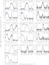 |
Fig. 2 APEX spectra of seven sources toward which the (0,0,0) and the (0, 11c, 0) HCN lines are detected. For each source, the upper and lower panels show the spectra for the (0,0,0) and the (0, 1 1c, 0) lines, respectively. Toward X Cnc and U Hya, only the (0,0,0) line could be detected, and its spectra are shown at the center and right in the bottom row. The vertical dotted blue line marks the stellar velocity, while the dashed blue lines indicate the terminal velocity. A TMB of 1 K corresponds to a flux density of 33.4 Jy. |
6.1.2 Hot HCN around IRC+10216
To place our results into context, we note that Cernicharo et al. (2011) studied a total of 63 J =3 → 2 rotational transitions from 28 vibrational states with energies of up to 10 700 K toward IRC+10216. Assuming local thermodynamic equilibrium (LTE) and using a rotation diagram (“Boltzmann plot”) analysis (their Fig. 2), these authors find the lines to arise from three temperature regimes, characterized by vibrational temperatures Tvib of ≈2465, 1240, and 410 K. The first of these is close to the effective temperature of 2750 K of the star inferred by Menten et al. (2012), and, together with the also determined column density, implies that HCN exists close to the stellar surface with an abundance relative to molecular hydrogen, x(HCN), of 5–7∕105. The extremely high excitation (~4500 K) laser lines discussed in Sect. 1 have widths consistent with an origin in this zone. Recent ALMA observations of lines from vibrationally excited HNC (hydrogen isocyanide) suggest that these exclusively originate from this innermost region (Cernicharo et al. 2013).
Over the second to the third zones (at 1240 and 420 K), which reside successively farther away from the star, x(HCN) drops by anorder of magnitude, and the FWHM line widths increase from the near-photospheric value of 5 km s−1 to 19 km s−1 in zone III. From visual inspection of spectra presented by Cernicharo et al. (2011), we find the FWZP of zone III lines to be ≈30 km s−1, identical to the value we find for our ν2 = 1 lines. The lines fitted by Cernicharo et al. (2011) in their Boltzmann plot, whose slopes yield the rotational temperatures or the three zones, represent all the observed data points fairly well. This shows that LTE is a good assumption for the populations of non-inverted, that is, of most, HCN levels throughout the innermost CSE of IRC+10216.
Tenenbaum et al. (2010) and Patel et al. (2011), for the HCN J = 3 → 2 and 4 → rotational lines confirm this dichotomy of narrow lines from highly excited vibrational states and broader lines from lower excitation states and the ground state.
Remarkably, both the strong (0, 11c, 0) maser and the weak (0, 11d, 0) line cover exactly the velocity range Cernicharo et al. (2011) determined for the zone III lines. Such broad widths, which correspond to twice the CSE terminal velocity, have been reported for vibrationally excited HCN lines before. The interpretation was that they arise from the entire region in which dust grains nucleate, and that consequently, the gas in the stellar outflow is accelerated from the stellar surface out to 20 r⋆ (Fonfría et al. 2008; Cernicharo et al. 2011; Cernicharo et al. 2013). This corresponds to 38 au, using the value of 1.9 au that Menten et al. (2012) have derived for r⋆, the radius of the stellar optical photosphere. These authors directly measured a diameter of 10.8 au (83 milliarcseconds) for the radio (and mm) photosphere of IRC+10216, which is significantly larger than the optical photosphere.
Results of HCN J = 2 → 1 line observations.
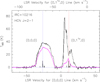 |
Fig. 3 Comparison of the spectra for the HCN J = 2 → 1 (0,0,0) and (0, 11c, 0) lines taken with the IRAM 30 m telescope in 1989 April by Lucas & Cernicharo (1989) (full line spectrum) and with the APEX 12 m telescope on 2015 May 28 (dotted magenta line spectrum). The bottom and top LSR velocity scales are appropriate for the (0,0,0) and the (0, 1 1c, 0) lines, respectively. Both spectra have a velocity resolution of 0.26 km s−1. The vertical bars give the relative intensities and velocities or the hfs components of the two lines. The intensity of the strongest component is normalized to TMB = 10 K. |
6.2 Other sources
As discussed in Sect. 3, for most sources, the (0, 1 1c, 0) line covers a much narrower velocity range than the (0,0,0) line and shows a variety of shapes. We now comment on this and other properties of selected sources.
In some sources the profile is dominated by one very narrow component, perhaps most clearly manifested in R For, which at our spectral resolution only appears in a few channels. This feature is most typical for maser lines, and it alone can be taken as indication for maser action. In addition to this narrow component, most sources show an underlying broader component that can have the form of a relatively smooth pedestal, like that in AI Vol, or an irregular shape. This broader component might represent thermal emission, but because of its intensity, in particular compared to that of the (0, 1 1d, 0) line, it is more likely a blend of several weaker maser spikes. Such features, which are also observed in other masing lines, may be highly variable and significantly change the overall appearance of the line profile with time. Except for V Hya (see Sect. 6.2.2), the velocity range covered by the broader component is much smaller than the full width of the (0,0,0) HCNline.
6.2.1 CIT 6 (RW LMi)
In some respects, CIT 6 appears to be a twin of IRC+10216. This pertains to their similar periods and terminal velocities, although the mass-loss rate of the latter object has been estimated to exceed the rate of CIT 6 by a significant factor. Nevertheless, if we scale the line fluxes of CIT 6 to those of IRC+10216 with the square of their distances, we obtain comparable values. In contrast to IRC+10216, the vibrationally excited lines cover a narrower velocity range toward CIT 6 than the (0,0,0) line.
We note that for CIT 6, the (0, 11c, 0) line has a higher peak brightness than the (0,0,0) line. The same is true for AI Vol (and for CQ Pyx both lines are comparable). In stark contrast, for another HCN maser line from an excited bending-mode state, much stronger emission was found from CIT 6 than from IRC+10216: Guilloteau et al. (1987) found the emission in the (0, 20, 0) J =1 → 0 line, the first HCN maser detected, to be ≈50 times stronger than in IRC+10216; see also Sect. 6.3.2.
6.2.2 V Hydrae
V Hya is a very evolved C-rich object that has been termed a “dying star”. It appears to be in a transitory state to a planetary nebula (Tsuji et al. 1988; Kahane et al. 1988; Sahai et al. 2003). Observations of lines observed at optical, IR, and millimeter wavelengths present a complex picture that has been interpreted as showing a high-velocity bipolar outflow (Kahane et al. 1996) together with an equatorial structure perpendicular to it (Sahai et al. 2003; Hirano et al. 2004).
As far as we know, our result for the HCN (0, 11c, 0) line represents the first detection of (sub)millimeter-wavelength rotational emission toward V Hya from highly excited energy levels. Quite remarkably, we measure a flux in this line that is comparable to the flux in the (0,0,0) line. Moreover, both lines cover comparable velocity ranges and have even similar profiles as the HCN J = 1 → 0 line observed with the Nobeyama 45 m telescope (Tsuji et al. 1988). These velocity ranges imply that this emission from all these lines arises from much of the acceleration region of this object’s outflow.
6.2.3 Other stars
Smith et al. (2014) summarized observations of maser emission in the (0, 20, 0) J = 1 → 0 line, which before had been detected in a total of nine sources. To this list they added V358 Lup (≡ IRAS 15082−4808, RAFGL 4211). Three of these objects are part of our sample, namely IRC+10216, CIT 6, and V358 Lup. Toward the last source, maser emission in this line had been observed to have a different appearance in 2010 and 2011 and was not detected at all in 1993. In 2011, a single feature was observed with a flux density of ≈4 Jy at a velocity that was a few km s−1 blueshifted from the stellar systemic velocity. In 2010, the intensity of this feature had been higher, ≈15 Jy, while lower-intensity emission had appeared at higher velocity. The total velocity range covered by this is smaller than that we observe in the J = 2 → 1 (0, 1 1c, 0) line, which has about twice the peak intensity of the (0, 20, 0) line. For V358 Lup and CIT 6, data also exist for multiple epochs. Neither source shows a propensity for stronger maser emission near ϕIR = 0 or weaker maser emission near ϕIR = 0.5.
6.3 Properties of the (0, 11c, 0) maser emission
6.3.1 Maser pumping
Based on observations of (non-masing) J = 2 − 1 (and other) rotational HCN lines from within several different vibrational states, Lucas & Cernicharo suggested that the (0, 1 1c, 0) maser could be explained by pumping into the v2 = 1 and 2 states via IR radiation at 14 and 7 μm, respectively.For radiative pumping to be feasible, the availability of at least one pump photon per maser photon is required. In Table 4 we compare the photon luminosities, Lph (M), in that line with the continuum photon luminosities in the 12 μm IRAS band, Lph (12 μm), for the 11 sources with detections inthe (0, 11c, 0) maser line. Values for the latter were calculated from the 12 μm flux densities listed in Table 2, scaled by the velocity range over which maser emission is observed, taken from Table 3. How does the 12 μm flux density compare to the 7 and 14 μm flux densities? Detailed modeling of IRC+10216’s wide band spectral energy distribution (SED), presented in the appendix of Menten et al. (2006), shows that it peaks between ≈8 and 10 μm (depending on its phase) and that its 7 and 14 μm flux densities are within a factor of 2 of the 12 μm flux density. Moreover, all these flux densities vary by less than a factor of 5 over the stellar pulsation cycle. Since IRC+10216’s Lph (12 μm) of 1.8∕1046 s−1 is greater by far than its Lph(M) of 3.9∕1042 s−1, it is safe to say that radiative pumping is certainly feasible in principle, even if the uncertainties discussed above are taken into account. This is also very likely true for the other stars in our sample, although detailed SED modeling is not available for them; in all cases, Lph (12 μm) ≫ Lph(M).
We would like to remark that the photon luminosities we determine for the HCN J = 2 − 1 (0, 1 1c, 0) maser line (Table 4) are comparable to or higher than typical values found for the strongest (J = 1 − 0 or 2 − 1) vibrationally excited (v = 1 or 2) SiO maser lines toward O-rich AGB stars.
6.3.2 Relation between maser flux and IR light curve
The flux of SiO masers around O-rich AGB stars shows a very close correlation with the IR light curve of these O-rich stars. The maser flux attains its maximum at visual phase between ≈0.05 and 0.2, that is, at or near the maximum of the IR light curve (see, e.g., Bujarrabal et al. 1987; Pardo et al. 2004).
Since only one of the HCN (0, 11c, 0) masers has been observed twice, we can only make very qualitative statements on the relation of its flux to the continuum flux from the star or its dust shell. The epoch when Lucas & Cernicharo (1989) first detected the (0, 1 1c, 0) and (0, 1 1d, 0) lines toward IRC+10216, 1989 April (Julian day, JD 2447631 ± 15), falls within the time range over which Le Bertre (1992) monitored the brightness of this star in multiple IR bands. Inspecting his published J, K, L, and M light curves, we estimate that the star was at IR phase, ϕIR = 0.23. For our own observations, which were made on JD 2457171, using the JD of IR maximum and the value for the period determined by Menten et al. (2012), we estimate ϕIR≈ 0.23, an identical value. Given that the maser luminosity was much stronger at the first epoch, this is very surprising.
A “decoupling” of IR light curve and maser variability has also been found for the (0, 20, 0) J =1 → 0 maser line observed toward IRAS 15082−4808 (RAFGL 4211) by Smith et al. (2014). For the few C-rich stars for which multiple observations of this line exist, these authors could not establish a propensity of stronger maser flux to appear at the IR maximum. The weakness of this line when it was first detected in IRC+10216 has been mentioned in Sect. 6.2.1. Multiple observations at different epochs have always found it at similarly weak (≈2 Jy) intensities and with similar (simple) line profiles (Lucas et al. 1986, 1988; Guilloteau et al. 1987; Lucas & Guilloteau 1992). This makes it doubtful whether this line shows maser action toward IRC+10216.
To explore this issue further, we note that other HCN lines from various vibrationally excited states show variability in IRC+10216 as well, but at a much lower level than the J =2 → 1 (0, 1 1d, 0) line (see Sect. 6.1.1 and Cernicharo et al. 2014; He et al. 2017). Cernicharo et al. (2014) observed the HCN J =6 → 5 (0, 1 1c, 0) and (0,0,0) lines with the Heterodyne Instrument for the Far Infrared (HIFI) on board the Herschel Space Observatory at two different times, on 2010 May and 2010 November, when the phase of the star was 0.23 and 0.53, respectively. On both dates, the J =6 → 5 (0,0,0) line shape was very similar to that of the J = 2 → 1 (0,0,0) line observed by us (see Sect. 6.1.1), while its total intensity decreased by 10% between the first to the second date. Changes in the J = 6 → 5 (0, 1 1c, 0) line were much more dramatic. On both dates, this line showed a sloping profile over most of the velocity range, which decreased in intensity from lower to higher velocities, in contrast to the profile we observed for the J =2 → 1 (0, 1 1c, 0) line, which peaksat the systemic velocity. Between 2010 May and November, the intensity of this broad emission decreased by a factor of ≈1.6 in total. On the two 2010 dates, a narrow spike is observed on the extreme blue edge of the line, whose excess intensity (over that of the broad emission) decreased in intensity even by a larger factor or ≈2. The intensity of a narrow spike at the redshifted edge diminished by an even larger amount. We note that the (0, 1 1c, 0) J = 2 → 1 line also had pronounced blueshifted emission when Lucas & Cernicharo (1989) observed it in 1989.
He et al. (2017) discussed the variability in the (0, 11d, 0) J = 3 → 2 line over the stellar (IR) cycle and considered different velocity ranges separately. While they found that the red portion of the profile remained constant, they discussed pronounced changes in its blue part that appeared to be correlated with the IR light. As one possibility to explain this, they suggested that the photospheric continuum emission might be amplified, which would require that the HCN maser were unsaturated. We note that the (0, 1 1c, 0) J = 2 → 1 line shows a very different profile at the two times it was observed, when the star was at identical phase and that the (0, 1 1c, 0) J = 6 → 5 line profile was different from both while also observed at this very same phase. This does not support background amplification, which, as discussed in Sect. 6.3.4, is generally rarely found to be associated with maser emission in AGB stars (see Sect. 6.3.4).
In conclusion, the flux of vibrationally excited HCN maser lines does not appear to be correlated with the stellar cycle, in contrast to the case of SiO masers around O-rich AGB stars. The reason for this is unclear, but we point out that the C-rich stars have mass-loss rates higher by more than an order of magnitude than O-rich AGB stars. This causes C-rich stars to have higher densities close to their photosphere than O-rich objects, possibly increasing the relative importance of collisional pumping for the former. In this context, it is interesting to note that Pardo et al. (2004) did not find any correlation between SiO maser and stellar phase for O-rich red supergiants, which have yet higher mass-loss rates than C-rich AGB stars.
In the case of SiO, the correlation of maser flux to stellar flux is frequently taken as evidence for radiative, rather than collisional pumping to cause the inversion (see, e.g., Pardo et al. 2004); both schemes have been discussed in the literature (Lockett & Elitzur 1992). Our results seem to indicate the possibility of a collisional pump for the vibrationally excited HCN masers discussed here. However, we point out that as discussed in Sect. 6.3.1, thereare abundant IR photons available to allow radiative pumping at any phase of the stellar variability cycle.
Comparison of HCN maser and IR photon luminosities.
6.3.3 Maser line widths
Under the assumption that the line width of narrow maser spikes in our observed spectra is determined by thermal broadening, we can derive a minimum temperature for the masing region. The kinetic temperature, Tkin, causing the thermal broadening of the profile of an HCN line to an FWHM Δ v, is given by
 (4)
(4)
where k is the Boltzmann constant, and the mass, m, of an HCN molecule is 27 atomic mass units. The narrowest features in our spectra have Δ v ≈ 0.6–1.2 km s−1 when we only determine the width of the narrow components that are superposed on broader emission; see Figs. 1 and 2. This corresponds to T = 215–844 K, which is broadly consistent with 410 K, the value Cernicharo et al. (2011) determine for zone III in IRC+10216 (see Sect. 6.1.2). We note that the above only provides a very qualitative estimate of the kinetic temperature and does not account for possible line narrowing that could occur for unsaturated maser lines. However, together with the fact that turbulence would broaden the lines, this makes it a lower limit of the actual temperature in the maser-emitting region.
As a consistency check, we note that using the Stefan-Boltzmann law and the luminosity of 8640 L⊙ determined by Menten et al. (2012) for IRC+10216, we derive a temperature of 614 K for a region of radius 38 au around this star. This is again comparable to the 410 K derived by Cernicharo et al. (2011), taking into account its variability.
We exclude line broadening caused by hyperfine structure. To illustrate this, the second strongest hfs component of the (0, 1 1c, 0) line has a an intrinsic intensity of 0.54 of that of the strongest and a velocity offset of +2.53 km s−1 relative to it. In sources with narrow features (Δ v ≲ 1 km s−1), for example, R For or RAFGL 4211 (Fig. 2), we do not find any feature at this velocity offset. This confirms the high-gain maser nature of this line emission: Exponential amplification of unsaturated maser emission with substantial gains very strongly favors the strongest hfs component and leaves intrinsically lower intensity components very weak and even undetectable in our case.
6.3.4 Constraints on the maser emission
As mentioned in Sect. 3, the peak emission in the (0, 1 1c, 0) maser line is slightly blueshifted relative to the systemic velocity for several of our sources, as is the (0, 20, 0) J = 1 → 0 maser line in RAFGL 4211; see Sect. 6.2.3. This effect would be naturally expected if the masing material were expanding away from the star and it would amplify the millimeter-wavelength continuum from the stellar photosphere. In reality, however, such amplification of photospheric continuum emission is rarely observed for circumstellar masers. It has recently been invoked by Gong et al. (2017) to explain the fact the blueshifted emission is variable and stronger than the redshifted emission for the J =1 → 0 line of SiS, whose maser nature they prove for IRC+10216.
High angular resolution observations of vibrationally excited SiO masers around O-rich AGB stars invariably show rings with sizes of a few r⋆ around the stars, indicating tangential amplification (see, e.g., Cotton et al. 2004; Reid & Menten 2007; Gray et al. 2009). Even more extreme, in the case of the archetypical M-type AGB star o Ceti (Mira), ALMA observations have recently shown redshifted absorption in vibrationally excited SiO lines (and one H2 O line) towardthe photosphere of the star, surrounded by rings of maser emission (Wong et al. 2016). By analogy, we conclude that simple inferences merely based on spectra are to be taken with caution for our HCN data, and high-resolution imaging with ALMA is required for an understanding of the complex up to a few tens of r⋆ -sized regions around C-rich AGB stars from which vibrationally excited HCN emission arises. So far, the physical conditions and (indirectly) the size of this region is only characterized by multiple high-excitation line spectroscopy (and not yet interferometry) and only forIRC+10216; see Sect. 6.1.2.
In Sect. 6.1.2 we have argued that for IRC+10216, the diameter of the emission region for both the strong (0, 1 1c, 0) maser and the (0, 1 1d, 0) line is the 76 au inferred by Cernicharo et al. (2013) from their modeling of HCN lines from various vibrational excited states. This corresponds to an angular size θS = 0”63 at the distance of this star. Taking this together with the peak main-beam brightness temperature of  = 14 K observed with the APEX telescope (see Fig. 1), we can use Eq. (3) to calculate a brightness temperature of TB = 46 000 K for the (0, 11c, 0) maser line. For this line, measured with the IRAM 30 m telescope by Lucas & Cernicharo (1989, see also our Fig. 3), we calculate TB = 43 000 K. These represent lower limits as the strongest maser emission may arise from a smaller region than assumed here. These values are higher than any value that would be consistent with thermal excitation, proving the maser nature of this line.
For the (0, 11d, 0) line ( K), we obtain a lower value of TB = 2600 K. Even this is significantly higher than the ≈400 K one would expect for an optically thick line from zone III (see Sect. 6.1.2). It likely implies weaker maser action in this line as well. Comparing the spectrum observed by us for this line with that observed by Lucas & Cernicharo (1989), we see marked changes, both in shape and intensity. In contrast to the strong (0, 1 1c, 0) maser line, we did not find dramatically stronger emission for the (0, 11d, 0) line in 2015 at velocities lower than the systemic value than in 1989, and despite the relatively low S/N of this line observed in 1989 with the IRAM telescope, we find a different profile with APEX. Moreover, for a compact source of size 0.′′ 63, one would expect
  , whereas we observe a value ≈1.5. This suggests significant variability in the (0, 11d, 0) line as well, supporting possible maser action.
7 Summary and outlook
Using the new ALMA Band 5 prototype receiver on the APEX 12-meter telescope, we conducted a survey for emission in the J = 2 → 1 rotational line from the (0,0,0), (0, 11c, 0), and (0, 11d, 0) vibrationally excited states of HCN toward a sample of 13 carbon-rich AGB stars. We detect broad thermally excited emission in the (0,0,0) line toward all of them and strong maser emission in the (0, 1 1c, 0) line toward a total of 11. Toward 4 of the latter, we also detect much weaker emission in the (0, 1 1d, 0) line. The velocity ranges covered by the vibrationally excited lines are consistent with their origin from within several stellar radii of the stellar photospheres, that is, in regions where the dust is still forming and the outflow is accelerating.
While it is clear that abundant IR photons are available to allow radiative pumping of the (0, 1 1c, 0) maser line, limited information on this and another vibrationally excited HCN maser line indicate a collisional pumping process. Temporally extended time monitoring of a sample of objects with the APEX telescope will shed light on the issue.
ALMA has now been fully equipped with Band 5 receivers and will allow interesting high angular resolution studies of all the J = 2 → 1 lines. ALMA high-resolution imaging with 15 km long baselines, which was available for the first (2014) ALMA Long Baseline Campaign (ALMA Partnership et al. 2015), can deliver synthesized beams with FWHM values of tens of milliarcseconds. This will allow resolving the radio photosphere of the nearby IRC+10216 and detailed imaging of the 0.′′ 6 diameter circumstellar region that contains vibrationally excited HCN, while ALMA data previously published by Cernicharo et al. (2013) with ≈ 0.′′6 do not yet allow such imaging. We note that since the other stars of our sample are much more distant than IRC+10216, imaging with the longest ALMA baseline is necessary to provide interesting constraints on the innermost regions of their envelopes. Moreover, continuum emission from the radio photospheres, while easily detectable at 177 GHz, will require higher-frequency imaging to be resolved.
Acknowledgements
D. Keller was supported for this research by the International Max-Planck-Research School (IMPRS) for Astronomy and Astrophysics at the Universities of Bonn and Cologne and the Bonn-Cologne Graduate School (BCGS) for Physics and Astronomy. We thank Ankit Rohatgi for making his WebPlotDigitizertool available as open source software. We are grateful to Javier Alcolea for comments and to Yan Gong, Christian Henkel, and the referee for reading the manuscript and their valuable comments. The referee is thanked for a meticulous job.
Appendix A Stellar phase determination
In order to derive the IR phases corresponding to the date of APEX observations, we required the corresponding periods and dates of a IR maximum, t0. While periods are relatively well known and published for most of our sources (Whitelock et al. 2006), t0 is generally not listed in the literature. We used the IR photometry from Whitelock et al. (2006) to independently derive t0 and the period for most of the APEX targets. Simple cosine curves were fitted using the least-squares method. Most derived periods were consistent with the published values; in cases when only few photometric points were available, the period was fixed at the value derived by Whitelock et al. (2006).
For two sources, X Cnc and U Hya, we could not find literature or archival IR data and instead used the information provided by AAVSO7 to derive their visual phases in the time of APEX observations. For most regular Mira variables, the IR light curve is delayed in phase by about 0.1 with respect to the visual phase. The phase could not be determined for X Tra and X Vel owing to the lack of information on the period and/or times of maxima.
Becausethe variability analysis here is based on scarce photometric data from cycles long in the past and the light curves often display a non-periodic component, the derived phases should be considered as very rough estimates.
References
- Adel, A., & Barker, E. F. 1934, Phys. Rev., 47, 277 [NASA ADS] [CrossRef] [Google Scholar]
- ALMA Partnership, Fomalont, E. B., Vlahakis, C., et al. 2015, ApJ, 808, L1 [Google Scholar]
- Avery, L. W., Bell, M. B., Cunningham, C. T., et al. 1994, ApJ, 426, 737 [NASA ADS] [CrossRef] [Google Scholar]
- Bieging, J. H. 2001, ApJ, 549, L125 [NASA ADS] [CrossRef] [Google Scholar]
- Billade, B., Nystrom, O., Meledin, D., et al. 2012, IEEE Trans. Terahertz Sci. Technol., 2, 208 [NASA ADS] [CrossRef] [Google Scholar]
- Bujarrabal, V., Planesas, P., & del Romero, A. 1987, A&A, 175, 164 [NASA ADS] [Google Scholar]
- Cernicharo, J., Yamamura, I., González-Alfonso, E., et al. 1999, ApJ, 526, L41 [NASA ADS] [CrossRef] [PubMed] [Google Scholar]
- Cernicharo, J., Agúndez, M., Kahane, C., et al. 2011, A&A, 529, L3 [NASA ADS] [CrossRef] [EDP Sciences] [Google Scholar]
- Cernicharo, J., Daniel, F., Castro-Carrizo, A., et al. 2013, ApJ, 778, L25 [Google Scholar]
- Cernicharo, J., Teyssier, D., Quintana-Lacaci, G., et al. 2014, ApJ, 796, L21 [NASA ADS] [CrossRef] [Google Scholar]
- Cherchneff, I. 2006, A&A, 456, 1001 [NASA ADS] [CrossRef] [EDP Sciences] [Google Scholar]
- Cotton, W. D., Mennesson, B., Diamond, P. J., et al. 2004, A&A, 414, 275 [NASA ADS] [CrossRef] [EDP Sciences] [Google Scholar]
- Cutri, R. M., Skrutskie, M. F., van Dyk, S., et al. 2003, 2MASS All Sky Catalog of Point Sources [Google Scholar]
- Dayal, A., & Bieging, J. H. 1995, ApJ, 439, 996 [NASA ADS] [CrossRef] [Google Scholar]
- Ebenstein, W. L., & Muenter, J. S. 1984, J. Chem. Phys., 80, 3989 [NASA ADS] [CrossRef] [Google Scholar]
- Feast, M. W., Glass, I. S., Whitelock, P. A., & Catchpole, R. M. 1989, MNRAS, 241, 375 [NASA ADS] [CrossRef] [Google Scholar]
- Fonfría, J. P., Cernicharo, J., Richter, M. J., & Lacy, J. H. 2008, ApJ, 673, 445 [NASA ADS] [CrossRef] [Google Scholar]
- Gong, Y., Henkel, C., Ott, J., et al. 2017, ApJ, 843, 54 [NASA ADS] [CrossRef] [Google Scholar]
- Gray, M. 2012, Maser Sources in Astrophysics (Cambridge: Cambridge University Press) [CrossRef] [Google Scholar]
- Gray, M. D., Wittkowski, M., Scholz, M., et al. 2009, MNRAS, 394, 51 [NASA ADS] [CrossRef] [Google Scholar]
- Gray, M. D., Baudry, A., Richards, A. M. S., et al. 2016, MNRAS, 456, 374 [NASA ADS] [CrossRef] [Google Scholar]
- Groenewegen, M. A. T., Barlow, M. J., Blommaert, J. A. D. L., et al. 2012, A&A, 543, L8 [NASA ADS] [CrossRef] [EDP Sciences] [Google Scholar]
- Groesbeck, T. D., Phillips, T. G., & Blake, G. A. 1994, ApJS, 94, 147 [NASA ADS] [CrossRef] [Google Scholar]
- Guilloteau, S., Omont, A., & Lucas, R. 1987, A&A, 176, L24 [NASA ADS] [Google Scholar]
- Güsten, R., Nyman, L. Å., Schilke, P., et al. 2006, A&A, 454, L13 [NASA ADS] [CrossRef] [EDP Sciences] [Google Scholar]
- He, J. H., Dinh-V-Trung, & Hasegawa, T. I. 2017, ApJ, 845, 38 [NASA ADS] [CrossRef] [Google Scholar]
- Hirano, N., Shinnaga, H., Dinh-V-Trung, et al. 2004, ApJ, 616, L43 [NASA ADS] [CrossRef] [Google Scholar]
- Humphreys, E. M. L., Immer, K., Gray, M. D., et al. 2017, A&A, 603, A77 [NASA ADS] [CrossRef] [EDP Sciences] [Google Scholar]
- Immer, K., Belitsky, V., Olberg, M., et al. 2016, The Messenger, 165, 13 [NASA ADS] [Google Scholar]
- Izumiura, H., Ukita, N., & Tsuji, T. 1995, ApJ, 440, 728 [NASA ADS] [CrossRef] [Google Scholar]
- Kahane, C., Audinos, P., Barnbaum, C., & Morris, M. 1996, A&A, 314, 871 [NASA ADS] [Google Scholar]
- Kahane, C., Maizels, C., & Jura, M. 1988, ApJ, 328, L25 [NASA ADS] [CrossRef] [Google Scholar]
- Klein, B., Philipp, S. D., Krämer, I., et al. 2006, A&A, 454, L29 [NASA ADS] [CrossRef] [EDP Sciences] [Google Scholar]
- Le Bertre, T. 1992, A&AS, 94, 377 [NASA ADS] [Google Scholar]
- Lockett, P., & Elitzur, M. 1992, ApJ, 399, 704 [NASA ADS] [CrossRef] [Google Scholar]
- Loup, C., Forveille, T., Omont, A., & Paul, J. F. 1993, A&AS, 99, 291 [NASA ADS] [Google Scholar]
- Lucas, R., & Cernicharo, J. 1989, A&A, 218, L20 [NASA ADS] [Google Scholar]
- Lucas, R., & Guilloteau, S. 1992, A&A, 259, L23 [NASA ADS] [Google Scholar]
- Lucas, R., Omont, A., Guilloteau, S., & Nguyen-Q-Rieu. 1986, A&A, 154, L12 [NASA ADS] [Google Scholar]
- Lucas, R., Omont, A., & Guilloteau, S. 1988, A&A, 194, 230 [NASA ADS] [Google Scholar]
- Maki, Jr. A. G., & Lide, Jr. D. R. 1967, J. Chem. Phys., 47, 3206 [NASA ADS] [CrossRef] [Google Scholar]
- Menten, K. M., Reid, M. J., Krügel, E., Claussen, M. J., & Sahai, R. 2006, A&A, 453, 301 [NASA ADS] [CrossRef] [EDP Sciences] [Google Scholar]
- Menten, K. M., Reid, M. J., Kamiński, T., & Claussen, M. J. 2012, A&A, 543, A73 [NASA ADS] [CrossRef] [EDP Sciences] [Google Scholar]
- Menzies, J. W., Feast, M. W., & Whitelock, P. A. 2006, MNRAS, 369, 783 [NASA ADS] [CrossRef] [Google Scholar]
- Morris, M., Zuckerman, B., Palmer, P., & Turner, B. E. 1971, ApJ, 170, L109 [NASA ADS] [CrossRef] [Google Scholar]
- Morris, M., Lucas, R., & Omont, A. 1985, A&A, 142, 107 [NASA ADS] [Google Scholar]
- Müller, H. S. P., Schlöder, F., Stutzki, J., & Winnewisser, G. 2005, J. Mol. Struct., 742, 215 [NASA ADS] [CrossRef] [Google Scholar]
- Nielsen, H. H. 1950, Phys. Rev., 78, 296 [NASA ADS] [CrossRef] [Google Scholar]
- Olofsson, H., Johansson, L. E. B., Hjalmarson, A., & Nguyen-Quang-Rieu 1982, A&A, 107, 128 [NASA ADS] [Google Scholar]
- Olofsson, H., Eriksson, K., Gustafsson, B., & Carlstrom, U. 1993, ApJS, 87, 267 [NASA ADS] [CrossRef] [Google Scholar]
- Olofsson, H., Lindqvist, M., Nyman, L.-A., & Winnberg, A. 1998, A&A, 329, 1059 [NASA ADS] [Google Scholar]
- Pardo, J. R., Alcolea, J., Bujarrabal, V., et al. 2004, A&A, 424, 145 [NASA ADS] [CrossRef] [EDP Sciences] [Google Scholar]
- Patel, N. A., Young, K. H., Gottlieb, C. A., et al. 2011, ApJS, 193, 17 [NASA ADS] [CrossRef] [Google Scholar]
- Reid, M. J., & Menten, K. M. 2007, ApJ, 671, 2068 [NASA ADS] [CrossRef] [Google Scholar]
- Rolffs, R., Schilke, P., Wyrowski, F., et al. 2011, A&A, 529, A76 [NASA ADS] [CrossRef] [EDP Sciences] [Google Scholar]
- Ryde, N., Schöier, F. L., & Olofsson, H. 1999, A&A, 345, 841 [NASA ADS] [Google Scholar]
- Sahai, R., Morris, M., Knapp, G. R., Young, K., & Barnbaum, C. 2003, Nature, 426, 261 [NASA ADS] [CrossRef] [PubMed] [Google Scholar]
- Sakamoto, K., Aalto, S., Evans, A. S., Wiedner, M. C., & Wilner, D. J. 2010, ApJ, 725, L228 [NASA ADS] [CrossRef] [Google Scholar]
- Salter, C. J., Ghosh, T., Catinella, B., et al. 2008, AJ, 136, 389 [NASA ADS] [CrossRef] [Google Scholar]
- Schilke, P., & Menten, K. M. 2003, ApJ, 583, 446 [NASA ADS] [CrossRef] [Google Scholar]
- Schilke, P., Mehringer, D. M., & Menten, K. M. 2000, ApJ, 528, L37 [NASA ADS] [CrossRef] [Google Scholar]
- Schöier, F. L., Ramstedt, S., Olofsson, H., et al. 2013, A&A, 550, A78 [NASA ADS] [CrossRef] [EDP Sciences] [Google Scholar]
- Smith, C. L., Zijlstra, A. A., & Fuller, G. A. 2014, MNRAS, 440, 172 [NASA ADS] [CrossRef] [Google Scholar]
- Snyder, L. E., & Buhl, D. 1971, ApJ, 163, L47 [NASA ADS] [CrossRef] [Google Scholar]
- Tenenbaum, E. D., Dodd, J. L., Milam, S. N., Woolf, N. J., & Ziurys, L. M. 2010, ApJ, 720, L102 [NASA ADS] [CrossRef] [Google Scholar]
- Thorwirth, S., Müller, H. S. P., Lewen, F., et al. 2003a, ApJ, 585, L163 [NASA ADS] [CrossRef] [Google Scholar]
- Thorwirth, S., Wyrowski, F., Schilke, P., et al. 2003b, ApJ, 586, 338 [NASA ADS] [CrossRef] [Google Scholar]
- Tsuji, T. 1964, Ann. Tokyo Astronom. Observ., 9, 1 [Google Scholar]
- Tsuji, T., Unno, W., Kaifu, N., et al. 1988, ApJ, 327, L23 [NASA ADS] [CrossRef] [Google Scholar]
- Veach, T. J., Groppi, C. E., & Hedden, A. 2013, ApJ, 765, L34 [NASA ADS] [CrossRef] [Google Scholar]
- Whitelock, P. A., Feast, M. W., van Loon, J. T., & Zijlstra, A. A. 2003, MNRAS, 342, 86 [NASA ADS] [CrossRef] [MathSciNet] [Google Scholar]
- Whitelock, P. A., Feast, M. W., Marang, F., & Groenewegen, M. A. T. 2006, MNRAS, 369, 751 [NASA ADS] [CrossRef] [EDP Sciences] [Google Scholar]
- Wong, K. T., Kamiński, T., Menten, K. M., & Wyrowski, F. 2016, A&A, 590, A127 [NASA ADS] [CrossRef] [EDP Sciences] [Google Scholar]
- Ziurys, L. M., & Turner, B. E. 1986, ApJ, 300, L19 [NASA ADS] [CrossRef] [PubMed] [Google Scholar]
See Sect. 4 for information on HCN spectroscopy.
We used the WebPlotDigitizer tool available on http://arohatgi.info/
All Tables
All Figures
|
Fig. 1 APEX spectra of the four sources toward which all three HCN J = 2 → 1 lines are detected. For each source, the upper, middle, and lower panels show the spectra for the (0,0,0), (0, 1 1c, 0), and (0, 11d, 0) lines, respectively. 1 K TMB corresponds to a flux density of 33.4 Jy. To facilitate the comparison between the lines, we used the same intensity scale for the first two lines, except for CW Leo. In addition, for CW Leo, the TMB scale of the dotted blue line shows the base of the (0, 11c, 0) spectrum scaled up by a factor of 8 compared to the ordinate in that panel. To adequately display the weak (0, 1 1d, 0) emission, a compressed TMB scale is used for all sources for this line. The vertical dotted blue line marks the stellar velocity, while the dashed blue lines indicate the terminal velocity. The spectral line partially appearing in the (0, 1 1d, 0) spectrum of IRC+10216 at velocities > 10 km s−1 is part of a multiplet component of the N = 18 → 17 transition of C3N. |
| In the text | |
|
Fig. 2 APEX spectra of seven sources toward which the (0,0,0) and the (0, 11c, 0) HCN lines are detected. For each source, the upper and lower panels show the spectra for the (0,0,0) and the (0, 1 1c, 0) lines, respectively. Toward X Cnc and U Hya, only the (0,0,0) line could be detected, and its spectra are shown at the center and right in the bottom row. The vertical dotted blue line marks the stellar velocity, while the dashed blue lines indicate the terminal velocity. A TMB of 1 K corresponds to a flux density of 33.4 Jy. |
| In the text | |
|
Fig. 3 Comparison of the spectra for the HCN J = 2 → 1 (0,0,0) and (0, 11c, 0) lines taken with the IRAM 30 m telescope in 1989 April by Lucas & Cernicharo (1989) (full line spectrum) and with the APEX 12 m telescope on 2015 May 28 (dotted magenta line spectrum). The bottom and top LSR velocity scales are appropriate for the (0,0,0) and the (0, 1 1c, 0) lines, respectively. Both spectra have a velocity resolution of 0.26 km s−1. The vertical bars give the relative intensities and velocities or the hfs components of the two lines. The intensity of the strongest component is normalized to TMB = 10 K. |
| In the text | |
Current usage metrics show cumulative count of Article Views (full-text article views including HTML views, PDF and ePub downloads, according to the available data) and Abstracts Views on Vision4Press platform.
Data correspond to usage on the plateform after 2015. The current usage metrics is available 48-96 hours after online publication and is updated daily on week days.
Initial download of the metrics may take a while.