© ESO 2018

1 Introduction

Testing Einstein’s general theory of relativity (GR) in the strong-field limit remains a difficult challenge. Recently, gravitational waves have been used to test GR’s predictions concerning merging black holes (see, e.g., Abbott et al. 2016), whose observations are consistent with GR and the existence of black holes (Chirenti & Rezzolla 2016). Building on Cunningham & Bardeen (1972), Falcke et al. (2000) suggested that a black hole’s “shadow” may be used to probe the accuracy of GR in the strong-field limit; observational efforts using millimeter-wavelength very long baseline interferometry (mm-VLBI) techniques are now underway (Falcke et al. 2000; Doeleman et al. 2008; Doeleman et al. 2012; Fish et al. 2016; Johnson et al. 2015; Goddi et al. 2016).

Prime motivating targets for this research are the putative accreting supermassive black holes (SMBHs) at the center of the Milky Way (Sagittarius A*, hereafter Sgr A*; Falcke & Markoff 2013; Genzel et al. 2010) and M 87 (Doeleman et al. 2012). The first attempts to predict the electromagnetic appearance of black holes were made in the 1970s (Cunningham & Bardeen 1972; Luminet 1979; Viergutz 1993), however, due to the limited observational capacity of that era, it was considered a somewhat academic exercise. With the advent of mm-VLBI techniques, and the potential to image the black-hole shadows in Sgr A*, efficient and flexible GR ray-tracing codes are becoming a key component of image-based tests of GR in the strong-field limit. It is no longer sufficient to calculate the appearance of thin disks or background stars, but rather, one has to consider a black hole surrounded by a heterogeneous, partially optically thick plasma. In order to accurately reproduce the appearance and spectrum of such a source to a distant observer, the effects of a strong gravitational field (gravitational lensing, redshift, and relativistic boosting) must be taken into account. For these reasons, creating synthetic observational data from physical models of the SMBH and its environment is an important component of the theoretical study of objects like Sgr A*.

Besides the study of SMBH’s, any astrophysical problem that involves radiative transfer and strong gravity could be tackled by general-relativistic radiative transfer codes. One example of such alternative applications is a binary black-hole system. For such systems, no analytical spacetime is known, and a numerical spacetime must be employed. Another example is the study of radiative transfer near neutron stars, for which, again, no exact metric is known (although it may be approximated by the Kerr metric, see, e.g., Parfrey & Tchekhovskoy 2017). Finally, a general-relativistic radiative transfer code could be applied to problems that do not involve compact objects, such as the propagation of radiation in an expanding FRW-spacetime.

Certain spacetimes, such as the Schwarzschild spacetime, are amenable to analytical solution of the geodesic equation (Beloborodov 2002; De Falco et al. 2016). A semi-analytical solution to the geodesic equation in the Kerr spacetime is presented by Dexter & Agol (2009). Analytical solutions to the geodesic equation near compact objects have also been studied in the context of, for example, radiating pulsars (Poutanen & Beloborodov 2006). Analytically or semi-analytically computed null geodesics have the important advantage of excellent spatial accuracy that is independent of integration step size. On the other hand, the analytical formulae may be expensive to evaluate, and thus a numerical code may, in some cases, offer superior performancewhen sensitive radiative-transfer calculations (which require a relatively small spatial integration step size) are included. Additionally, analytical codes are restricted to the set of spacetimes for which the metric and connection are known analytically.

Numerical radiative-transfer codes, capable of producing images and/or spectra from general relativistic magneto-hydrodynamical (GRMHD) simulations by performing radiative-transfer calculations in strong gravity, have been studied in a number of works (Broderick 2006; Noble et al. 2007; Dexter & Agol 2009; Shcherbakov & Huang 2011; Chan et al. 2013; Dexter 2016). Dexter (2016)’s grtrans is a CPU-based code that uses a semi-analytic method to construct geodesics and offers polarized radiative transfer in the Kerr spacetime; Moscibrodzka & Gammie (2018)’s ipole is a numerical code that offers the same functionality, but for general spacetimes. Chan et al. (2013)’s GRay is a fully numerical GPU-based CUDA code capable of handling arbitrary spacetime metrics; it was recently succeeded by GRay2, a general-purpose geodesic integrator for the Kerr spacetime (Chan et al. 2017). Takahashi & Umemura (2017) have recently presented ARTIST, a code that is not based on a ray-tracing algorithm, but which is capable of reproducing radiation fields (wave fronts) in the Kerr spacetime, with the aim of including radiation pressure in GRMHD simulations. Although both GPU and CPU codes that perform radiative-transfer calculations are available, existing codes are specialized to one or the other. Many are also restricted to hardware from a single manufacturer, so that deciding which code to use may strongly depend on the hardware available locally.

In this paper, we present a new code, RAPTOR. It was designed with two goals in mind: minimizing the number of physical assumptions, by supporting arbitrary spacetimes and time-dependent radiative transfer, and maximizing flexibility of use, by supporting all commonly available CPU and GPU hardware. Although the code was developed with the science case described above in mind, it may be readily applied to any astrophysical problem involving radiative transfer in strong gravity, as it is equipped to deal with numerical as well as analytical metrics. One alternative application for the code that we have explored in particular concerns visualisation of black holes in virtual reality, a project that has applications in outreach and intuitive understanding of black hole accretion (Davelaar et al., in prep.). Presently, we only compute the specific intensity as seen by the observer. The next step, which involves polarized radiative transfer, will be covered in a future paper. In this work, we demonstrate correct operation of RAPTOR and couple it to GRMHD simulation data from BHAC (Porth et al. 2017) and HARM2D (Gammie et al. 2003) using radiative-transfer models (Mościbrodzka et al. 2009). We also perform a detailed comparison with the radiative-transfer code BHOSS (Younsi, in prep.) by specifying identical initial conditions in both codes and comparing the resulting images. Finally, in order to evaluate the accuracy of theoretical predictions of the appearance and time-variability of SMBH accretion flows, we apply our new code to studying the slow-light paradigm, in which the assumption of staticity of GRMHD data is relaxed, in the context of accreting black holes. The paper is organized as follows: in Sect. 2, we present the governing equations for calculating (null) geodesics in a curved spacetime, derive two algorithms for solving them numerically, and test our implementations. In Sect. 3, we discuss the covariant radiative-transfer equation and the accompanying numerical algorithms for solving it. Section 4 contains a library of verification and performance results for the geodesic and radiative-transfer integrators. In Sect. 5, we apply RAPTOR to investigate the slow-light paradigm for imaging GRMHD simulations.

2 Equations of motion for light rays

The appearance and spectrum of an accreting black hole recorded by a distant observer are strongly affected by gravitational effects such as lensing and redshift. In order to construct an accurate image or spectrum, these effects must be taken into account. Relativistic ray-tracing algorithms solve the equations of motion for light in curved spacetime, automatically taking into account all gravitational effects. Such algorithms are discussed in this section.

2.1 Geodesic equation

In Newtonian physics, test particles move along straight lines in the absence of any force. Analogously, in GR, test particles move along so-called geodesics when in free fall, in other words, when acted upon by gravity only. Furthermore, in GR gravitational effects on test particles are represented through curvature of the spacetime in which the particles move.

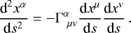
The structure of spacetime in GR is described by the symmetric rank-2 metric tensor g_μν and the motion of test particles is described by the geodesic equation $$\frac{{\text{d}}^2{x}^{\alpha }}{\text{d}{s}^2}=-{\Gamma }_{\mu \nu }^{\alpha }\frac{\text{d}{x}^{\mu }}{\text{d}s}\frac{\text{d}{x}^{\nu }}{\text{d}s}.$$(1)

Here, x^α is the particle’s position; s is a scalar parameter of the particle’s world line, and ${\Gamma }_{\mu \nu }^{\alpha }$ is the “connection” of the spacetime through which the particle propagates. The connection depends on first derivatives of the metric and is given by $${\Gamma }_{\mu \nu }^{\alpha }=\frac{1}{2}{g}^{\alpha \rho }\left[{\partial }_{\mu }{g}_{\nu \rho }+{\partial }_{\nu }{g}_{\mu \rho }-{\partial }_{\rho }{g}_{\mu \nu }\right].$$(2)

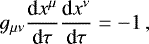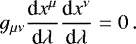
Massive particles move along “timelike” geodesics. Adopting the Lorentzian metric signature (−, +, +, +) and geometrized units, so that G = c = 1, the spacetime interval for massive particles of unit mass is negative and unitary: $$g_{\mu \nu }\frac{\text{d}{x}^{\mu }}{\text{d}\tau }\frac{\text{d}{x}^{\nu }}{\text{d}\tau }=-1,$$(3) where τ is the proper time measured by an observer co-moving with the particle. Photons, which are massless and always travel at the speed of light, travel along “null” geodesics with zero spacetime interval: $$g_{\mu \nu }\frac{\text{d}{x}^{\mu }}{\text{d}\lambda }\frac{\text{d}{x}^{\nu }}{\text{d}\lambda }=0.$$(4)

In this case, the geodesic is parametrized by a so-called affine parameter λ, as no proper time elapses for photons. From now on, we only consider null geodesics.

2.2 Numerical integration of the geodesic equation

In this section we present two algorithms to solve Eq. (4) numerically, and discuss a number of tests of the integrator’s performance.

Since the geodesic Eq. (1) represents a set of four coupled second-order ordinary differential equations (ODE’s), we must specify both an initial position $x_0^{\alpha }$ and an initial contravariant four-momentum vector, which in the case of radiation is the so-called wave vector $k_0^{\alpha }$, to obtain the full geodesic by numerical integration. As a first step, we can write Eq. (1) as a system of eight coupled first-order ODE’s: $$\begin{array}{lll}\frac{\text{d}{x}^{\alpha }}{\text{d}\lambda }\hfill & =\hfill & k^{\alpha },\hfill \\ \frac{\text{d}{k}^{\alpha }}{\text{d}\lambda }\hfill & =\hfill & -{\Gamma }_{\mu \nu }^{\alpha }{k}^{\mu }{k}^{\nu }.\hfill \end{array}$$

We must now choose an appropriate integration scheme to solve Eq. (5). Since we aim to strike a balance between accuracy and efficiency, we present two alternatives, one of which is more accurate while the other is less computationally expensive.

2.2.1 Runge-Kutta integrator

We first choose the popular 4th-order Runge-Kutta integration method (RK4) to solve Eq. (5) numerically. In the case of the geodesic equation there are eight dependent variables (the components of x^α and k^α), and we must evaluate 32 “update coefficients" for the RK4 integration: 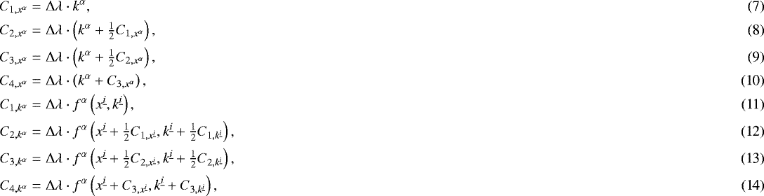$$\begin{array}{lll}{C}_{1,x^{\alpha }}\hfill & =\hfill & \Delta \lambda \cdot k^{\alpha },\hfill \\ C_{2,x^{\alpha }}\hfill & =\hfill & \Delta \lambda \cdot \left(k^{\alpha }+\frac{1}{2}{C}_{1,x^{\alpha }}\right),\hfill \\ C_{3,x^{\alpha }}\hfill & =\hfill & \Delta \lambda \cdot \left(k^{\alpha }+\frac{1}{2}{C}_{2,x^{\alpha }}\right),\hfill \\ C_{4,x^{\alpha }}\hfill & =\hfill & \Delta \lambda \cdot \left(k^{\alpha }+C_{3,x^{\alpha }}\right),\hfill \\ C_{1,k^{\alpha }}\hfill & =\hfill & \Delta \lambda \cdot f^{\alpha }\left(x^{\underset{\_}{i}},k^{\underset{\_}{i}}\right),\hfill \\ C_{2,k^{\alpha }}\hfill & =\hfill & \Delta \lambda \cdot f^{\alpha }\left(x^{\underset{\_}{i}}+\frac{1}{2}{C}_{1,x^{\underset{\_}{i}}},k^{\underset{\_}{i}}+\frac{1}{2}{C}_{1,k^{\underset{\_}{i}}}\right),\hfill \\ C_{3,k^{\alpha }}\hfill & =\hfill & \Delta \lambda \cdot f^{\alpha }\left(x^{\underset{\_}{i}}+\frac{1}{2}{C}_{2,x^{\underset{\_}{i}}},k^{\underset{\_}{i}}+\frac{1}{2}{C}_{2,k^{\underset{\_}{i}}}\right),\hfill \\ C_{4,k^{\alpha }}\hfill & =\hfill & \Delta \lambda \cdot f^{\alpha }\left(x^{\underset{\_}{i}}+C_{3,x^{\underset{\_}{i}}},k^{\underset{\_}{i}}+C_{3,k^{\underset{\_}{i}}}\right),\hfill \end{array}$$ where f^α represents the right-hand side of Eq. 1, and $\underset{\_}{i}$ is a shorthand indicating that all components of x^α and k^α appear as variables of f^α, i.e. $f^{\alpha }\left(x^{\underset{\_}{i}},k^{\underset{\_}{i}}\right)=f^{\alpha }\left(x^1,x^2,x^3,x^4,k^1,k^2,k^3,k^4\right)$. Having calculated all update coefficients using Eq. 14, we can compute the new values for x^α and k^α as follows: $$\begin{array}{lll}{x}_{\text{new}}^{\alpha }\hfill & =\hfill & x^{\alpha }+\frac{1}{6}\left(C_{1,x^{\alpha }}+2C_{2,x^{\alpha }}+2C_{3,x^{\alpha }}+C_{4,x^{\alpha }}\right)+O\left(\Delta {\lambda }^5\right),\hfill \\ k_{\text{new}}^{\alpha }\hfill & =\hfill & k^{\alpha }+\frac{1}{6}\left(C_{1,k^{\alpha }}+2C_{2,k^{\alpha }}+2C_{3,k^{\alpha }}+C_{4,k^{\alpha }}\right)+O\left(\Delta {\lambda }^5\right).\hfill \end{array}$$

2.2.2 Verlet integrator

Although the RK4 integrator is accurate, more efficient integrators exist. Evaluating the connection coefficients is the most computationally expensive operation in our geodesic integration algorithms; structuring our code in this manner allows us to maintain a general scheme that is capable of interfacing with GRMHD simulations in different coordinate systems, as well as of handling spacetimes that are completely arbitrary such as those in the framework of Rezzolla & Zhidenko (2014) and Konoplya et al. (2016), and recently employed by Younsi et al. (2016). Dolence et al. (2009) have presented the velocity Verlet algorithm (Swope et al. 1982) as a more efficient alternative to the RK4 algorithm, as it relies on fewer evaluations of the connection coefficients: $$\begin{array}{l}{x}_{n+1}^{\alpha }=x_n^{\alpha }+k_n^{\alpha }\Delta \lambda +\frac{1}{2}{\left(\frac{\text{d}{k}^{\alpha }}{\text{d}\lambda }\right)}_n{\left(\Delta \lambda \right)}^2\text{},\\ k_{n+1,p}^{\alpha }=k_n^{\alpha }+{\left(\frac{\text{d}{k}^{\alpha }}{\text{d}\lambda }\right)}_n\Delta \lambda ,\\ {\left(\frac{\text{d}{k}^{\alpha }}{\text{d}\lambda }\right)}_{n+1}=-{\Gamma }_{\mu \nu }^{\alpha }\left(x_{n+1}^{\alpha }\right)k_{n+1,p}^{\mu }{k}_{n+1,p}^{\nu },\\ k_{n+1}^{\alpha }=k_n^{\alpha }+\frac{1}{2}\left[{\left(\frac{\text{d}{k}^{\alpha }}{\text{d}\lambda }\right)}_n+{\left(\frac{\text{d}{k}^{\alpha }}{\text{d}\lambda }\right)}_{n+1}\right]\Delta \lambda .\end{array}$$

The accuracy of this algorithm can be improved by using the result of Eq. (20) to recompute the derivative (Eq. (19)) with $k_{n+1,p}^{\mu }=k_{n+1}^{\mu }$, and then reevaluating Eq. (20).

In this paper we have restricted our investigations to the Kerr spacetime, which represents an uncharged black hole with (in the general case) non-zero angular momentum characterized by the spin parameter a := J∕M², where J is the black-hole’s angular momentum and M its mass. Near the black-hole event horizon, as well as near the symmetry axis (the spin axis), numerical integration becomes difficult due to coordinate singularities. The following adaptive step-size routine introduced by Noble et al. (2007) and Dolence et al. (2009) is adopted for accuracy and efficiency in difficult regions by reducing the step-size Δ λ in these cases: $$\begin{array}{lll}\text{d}\lambda \hfill & =\hfill & \frac{1}{{\left|\text{d}{\lambda }_{x^1}\right|}^{-1}+{\left|\text{d}{\lambda }_{x^2}\right|}^{-1}+{\left|\text{d}{\lambda }_{x^3}\right|}^{-1}},\hfill \end{array}$$(21) where $$\begin{array}{lll}\text{d}{\lambda }_{x^1}\hfill & :=\hfill & ϵ/\left(\left|k^r\right|+\delta \right)\text{},\hfill \\ \text{d}{\lambda }_{x^2}\hfill & :=\hfill & ϵ\text{\hspace{0.17em}min}\left(x^{\theta },1-x^{\theta }\right)/\left(\left|k^{\theta }\right|+\delta \right)\text{},\hfill \\ \text{d}{\lambda }_{x^3}\hfill & :=\hfill & ϵ/\left(\left|k^{\varphi }\right|+\delta \right)\text{}.\hfill \end{array}$$

Here, δ is a very small (positive) number that protects against dividing by 0, while ϵ is a (positive) scaling parameter by which one can influence the scale of all steps.

2.3 Initial conditions: the virtual camera

Specific to the case of a Kerr black hole, consider a distant observer whose inclination angle with respect to the black-hole rotation axis is given by i so that an inclination angle of 90° means the observer is in the black-hole equatorial plane, while an inclination angle of 0° means that we are looking at the black hole along the direction of its spin axis. In the observer’s image plane, which is oriented so that its vertical axis is aligned with the black-hole spin axis (for any non-zero inclination angle), we define the impact parameters α (the distance from the black-hole rotation axis) and β (the distance in the direction perpendicular to α). The wave vector k^α is then constructed following Cunningham & Bardeen (1972) as $$\begin{array}{lll}L\hfill & =\hfill & -\alpha E\sqrt{1-{\cos }^{2}i},\hfill \\ Q\hfill & =\hfill & E^2\left[{\beta }^2+{\cos }^{2}i\left({\alpha }^2-1\right)\right]\text{},\hfill \\ k_t\hfill & =\hfill & -E,\hfill \\ k_{\varphi }\hfill & =\hfill & L,\hfill \\ k_{\theta }\hfill & =\hfill & \text{sign}(\beta )\sqrt{\left|Q-L^2{\cot }^2\theta +E^2{\cos }^2\theta \right|},\hfill \end{array}$$ where E is the wave vector’s total energy, L is the projection of the angular momentum parallel to the black- hole spin axis, and Q is the Carter constant (Carter 1968). The radial component of the wave vector, k^r, is fixed by demanding that it is a null vector, that is, k_αk^α = 0 (k^r may be positive or negative, corresponding to out- and ingoing rays, respectively). Boyer-Lindquist (BL) coordinates (Boyer & Lindquist 1967) are used to construct the initial wave vector.

2.4 Coordinate systems and transformations

One of the main purposes of RAPTOR is to integrate the radiative-transfer problems generic black-hole spacetimes such as those proposed in alternative to GR theories of gravity (Rezzolla & Zhidenko 2014). Hence, null-geodesic integration and the radiative-transfer equations described in the next section are formulated in a way that is independent of the choice of coordinate system or of the geometry of the spacetime. In view of this, RAPTOR has been constructed so as to switch easily among various grids and geometries. In particular, when considering the solution of the radiative-transfer equation near black holes, it is important that the coordinate system is accurate near the horizon, and compatible with GRMHD simulations; the latter customarily adopt a spherical-polar coordinate system using a logarithmic scale for the radial coordinate and a denser polar coordinate mapping near the equatorial plane (so-called modified coordinate systems, see, e.g., Gammie et al. 2003). In this paper, we utilized four different coordinate systems for the Kerr spacetime, namely: the aforementioned Boyer-Lindquist coordinates, the modified Boyer-Lindquist (MBL) coordinates, the logarithmic Kerr-Schild (KS) coordinates (Kerr & Schild 1965), and the modified Kerr-Schild (MKS) coordinates (Gammie et al. 2003). Some of the transformation laws between these coordinate systems are given explicitly in Appendix A, while a test of the code performance is presented in Appendix B.

3 Radiative transfer

Having previously computed the relevant null geodesics, an algorithm is needed that will perform radiative-transfer calculations along them. In this section we introduce the relevant equations. Our present algorithm does not include radiation refraction effects due to the plasma (which is a good approximation if the radiation frequency is greater than the plasma frequency, 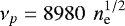${\nu }_p=8980n_{\text{e}}^{1/2}$, where n_e is the electron number density), all forms of scattering, and polarization although all of these effects can be incorporated in a ray-tracing simulations (see, e.g., Broderick 2006; Dolence et al. 2009; or Dexter 2016). However, RAPTOR integrates the radiative transfer equations taking into account changes in the plasma structure during the light transport (Sect. 5), which is usually neglected. Hence, our code is suitable for first-principles study of time variability of mock observations of accreting black holes or any other compact objects surrounded by plasma.

3.1 Covariant radiative-transfer equation

The transfer equation for the Lorentz invariant quantity I_ν∕ν³, where I_ν is the specific intensity of radiation at frequency ν, is given by (Lindquist 1966): $$\frac{\text{d}}{\text{d}\lambda }\left(\frac{I_{\nu }}{{\nu }^3}\right)=\frac{j_{\nu }}{{\nu }^2}-\nu {\alpha }_{\nu }\left(\frac{I_{\nu }}{{\nu }^3}\right),$$(30) where again λ is the affine parameter, which we defined to be increasing as the ray travels from the plasma toward the observer, ν is the photon’s frequency, j_ν is the plasma emission coefficient, and α_ν is the plasma absorptivity. We note that all of these physical quantities are computed in an inertial frame that is co-moving with the plasma (hereafter the fluid frame). In the present case of unpolarized radiative transfer, the necessary transformation between frames can be achieved simply by computing the ray’s frequency in the fluid frame: $$\nu =-k^{\alpha }{u}_{\alpha },$$(31) and using ν to relate the fluid frame emission and absorption coefficients to their Lorentz-invariant counterparts, so that we do not have to construct the fluid frame explicitly, as is the case with polarized radiative transfer.

The intensity seen by the observer, $I_{\nu ,\text{obs}}=I_{\nu }\left({\lambda }_{\text{obs}}\right)$, is then obtained by integrating Eq. (30) from λ₀ to λ_obs and subsequently converting from the Lorentz-invariant quantity I_ν∕ν³ to the specific intensity in the observer frame using $$I_{\nu ,\text{obs}}=\frac{I_{\nu }}{{\nu }^3}{\nu }_{\text{obs}}^3.$$(32)

Although it is possible to integrate Eq. (30) directly, more accurate numerical results can be obtained by employing the formal solution to the transfer equation (see e.g., Dexter & Agol 2009), which recasts I_ν as a function of the optical depth τ_ν given by: $${\tau }_{\nu }\left(\lambda \right)={\displaystyle {\int }_{{\lambda }_0}^{\lambda }\nu }{\alpha }_{\nu }\text{d}{\lambda }^{\prime }.$$(33)

We note that the optical depth, which describes the fraction of photons that pass through a certain absorbing volume, is a Lorentz-invariant quantity. The formal solution to the radiative-transfer equation is then $$\frac{I_{\nu }}{{\nu }^3}\left({\tau }_{\nu }\right)=\frac{I_{\nu }}{{\nu }^3}\left({\tau }_{\nu ,0}\right)\exp \left(-{\tau }_{\nu }\right)+{\displaystyle {\int }_{{\tau }_{\nu ,0}}^{{\tau }_{\nu }}\exp }-\left({\tau }_{\nu }-{\tau }_{{\nu }^{\prime }}\right)\frac{j_{\nu }}{{\nu }^3{\alpha }_{\nu }}\text{d}{\tau }_{{\nu }^{\prime }},$$(34) where τ_ν,0 defines the location along the null geodesic where integration begins. We can repeatedly solve Eq. (34) for each integration step. Assuming that j_ν is constant over the step, we obtain $$\frac{I_{\nu }}{{\nu }^3}\left({\tau }_{\nu }\right)=\frac{I_{\nu }}{{\nu }^3}\left({\tau }_{\nu ,0}\right)\exp \left(-{\tau }_{\nu }\right)+\frac{j_{\nu }}{{\nu }^3{\alpha }_{\nu }}\left(1-\exp \left(-{\tau }_{\nu }\right)\right).$$(35)

The reason for which using Eq. (35) yields better numerical results than direct integration of Eq. (30) with, for example,an explicit Euler scheme, is that in the latter case, the intensity may become negative if we take too large an integration step whenever $j_{\nu }/{\nu }^2<\nu {\alpha }_{\nu }\left(I_{\nu }/{\nu }^3\right)$, thus producing grossly incorrect results. Equation (34), on the other hand, contains an integrand that is always positive.

An evenmore numerically advantageous method for calculating the intensity seen by the observer can be obtained by integrating I_ν,obs in the opposite direction along the null geodesic with respect to the previous schemes, in other words, from the observer toward the plasma, by splitting Eq. (35) into separate equations for I_ν and τ_ν (Younsi et al. 2012). In fact, in this direction, I_ν,obs must be a monotonically increasing function of the affine parameter $\overline{\lambda }$, which we defined to increase in the opposite spatial direction of the previously used affine parameter λ ($\overline{\lambda }$ increases as the ray travels further away from the observer). This is because the specific intensity of the ray seen by the observer can only increase, never decrease, by continued integration further away from the camera (see Figs. 1 and 2 for an illustration of the difference between the two strategies).

This method offers three additional advantages over the two methods described above. Firstly, it allows simultaneous integration of the null geodesic and of the specific intensity, as well as cutting off the null-geodesic integration when the optical depth of thematerial between the current location and the camera becomes higher than a threshold value (any radiation emitted beyond this point will be severely attenuated and thus be negligible for the observer). Secondly, it relieves the need for a data structure to store the geodesic in memory before performing radiative-transfer calculations (since we simply integrate I_ν,obs along with the geodesic itself). Thirdly, with this method, it is possible to compute appropriate integration step-sizes for both thenull geodesic and the radiative-transfer integration, and then pick the minimum of the two. This avoids situations where the null-geodesic integration, performed separately as if in a vacuum, takes a large step through a plasma that is optically thick at a range of frequencies of interest, yielding inaccurate radiative-transfer calculations.

An expression for I_ν,obs can be constructed by considering a ray travelling backward from the camera into a radiating plasma. At each point along the ray’s path, we computed the optical depth of the material between the current location, λ, and the observer’s location, λ_obs as $${\tau }_{\nu ,\text{obs}}\left(\lambda \right)={\displaystyle {\int }_{{\lambda }_{\text{obs}}}^{\lambda }{\alpha }_{\nu }}({\lambda }^{\prime })\nu \text{\hspace{0.17em}d}{\lambda }^{\prime }.$$(36)

We can then compute the local invariant emission coefficient, $\left(j_{\nu }/{\nu }^2\right)$, and scale it by $\exp \left(-{\tau }_{\text{obs}}\right)$, resulting in the following expression for the contribution of point λ on the geodesic to the total observed intensity: $$\frac{\text{d}}{\text{d}\overline{\lambda }}\left(\frac{I_{\nu ,\text{obs}}}{{\nu }_{\text{obs}}^3}\right)=\frac{j_{\nu }}{{\nu }^2}\exp \left(-{\tau }_{\nu ,\text{obs}}\left(\overline{\lambda }\right)\right).$$(37)

Integrating over the geodesic then yields the total invariant intensity at the observer, $I_{\nu ,\text{obs}}/{\nu }_{\text{obs}}^3$, which is converted to I_ν,obs using Eq. (32) as before.

We have implemented all three integration strategies discussed in this section in RAPTOR and found that integration of Eq. (37) produces the most accurate results in the least amount of time.

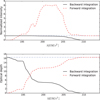Fig. 1 Radiative-transfer variables along a particular null geodesic that intersects a radiating plasma near a Kerr black hole (see Fig. 2). Top: local specific intensity Iν (dashed red curve), which is computed by integrating Eq. (34) in the direction of increasing affine parameter λ, and of the specific intensity seen by the observer, Iν,obs (solid black curve), which is computed by integrating Eq. (37) in the direction of decreasing λ. The intensity is normalized with respect to the observed intensity in both cases, so that we expect both curves to approach unity with continued integration, which is illustrated using the blue guideline. We note that Iν is a non-monotonic function of λ while Iν,obs is a monotonic function of λ. We also notethat for Iν,obs and τν,obs, integration proceeds from right to left in these plots, and that Iν,obs converges much faster than Iν. Bottom: optical depth for the same ray.

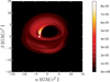Fig. 2 Synchrotron emission map created using a GRMHD simulation (see Sect. 4.2.2) made using the HARM code (Gammie et al. 2003). Intensity is given in units of Jy pixel−2. The observer frequency is 100 GHz, the inclination angle is 30 degrees, and the disk-dominated emission model discussed in Sect. 5 is used. Note the optically-thick accretion disk and strong emission to the left of the black-hole shadow (this region appears bright due to relativistic beaming). The ray investigated in Fig. 1 is marked by a white dot in this image. This particular ray, travelling from the plasma to the observer, first passes through the bright, relativistically-boosted region, and then through an optically-thick, non-boosted region of the disk, suggesting that the specific intensity along this ray will sharply increase, then decrease, before reaching the observer. Figure 1 shows that this is indeed the case.

4 Code verification

Since the program consists of two parts, namely the integration of the geodesics and the integration of the radiative-transfer equation, correct results must be verified for both. In Sect. 4.1 we verify the correct integration of null geodesics, while in Sect. 4.2 we focus on the radiative-transfer computations.

4.1 Verification of geodesic integration

In his seminal work, Carter (1968) presented three conserved quantities associated with the orbits of photons (or particles) in the Kerr spacetime: $$\begin{array}{lll}E\hfill & =\hfill & -k_t,\hfill \\ L\hfill & =\hfill & k_{\varphi },\hfill \\ Q\hfill & =\hfill & k_{\theta }^2+{\cos }^2\theta \left[a^2\left({\mu }^2-k_t^2\right)+k_{\varphi }^2/{\sin }^2\theta \right]\text{},\hfill \end{array}$$ where Q is the so-called Carter constant. Figure 3 shows, in terms of the L₁ -error norms, that these quantities are conserved as expected and that the errors converge respectively to second and fourth order in step-size for the Verlet and RK4 algorithms, for all coordinate systems.

Another interesting test for the geodesic integration comes from considering those null geodesics in the Kerr spacetime that have a complex morphology, looping around the horizon many times before plunging in or escaping. Such pathological geodesics are a good test for the code’s performance in a worst-case scenario because even small errors lead to deviations (e.g., absorption into the event horizon). Table 1 shows the parameters for two such geodesics.

Since geokerr is a semi-analytical code, it provides an excellent reference for the accuracy of a numerical scheme. Plots of the null geodesics described in Table 1, produced by both geokerr and RAPTOR, are shown in Fig. 4.

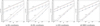Fig. 3 Convergence plots for the L1-error norms of the conserved quantities E (dashed blue), L (solid black), and Q (dotted red) for the orbit with parameters i = 90°, α = −3.22, β = 1.12, a = 0.998 with different integrator settings. The errors are computed at a fixed coordinate time tfinal. Two guide lines with slopes −2 (solid) and −4 (dashed) are drawn. The +, −, and ×-symbols represent respectively L, Q, and E, for the RK4integrator. The square, hexagon, and circle symbols represent the same quantities for the Verlet integrator.

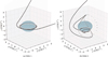Fig. 4 Comparison of null geodesics computed by the semi-analytical integrator geokerr to those computed by our fully numerical code. In each case, the geodesic represented by the black dots was computed using geokerr while the geodesic represented by the white dotted line is the output of RAPTOR (dots were chosen for the former geodesic because its variable step-size can otherwise create interpolation issues). The gray spheroid represents the black hole’s outer event horizon. MKS coordinates were used with ϵ = 0.001. The parameters for these geodesics are listed in Table 1.

4.2 Verification of radiative-transfer calculations

4.2.1 Emission line profiles and images of a thin accretion disk

The first model we investigated revolves around line emission profiles emitted from a thin accretion disk, which has been studied by, among others, Luminet (1979) and Laor (1991), and reproduced in Schnittman & Bertschinger (2004, see also Schnittman & Rezzolla 2006, and Dexter & Agol 2009). The model involves a steady state, optically thick, geometrically thin accretion disk which is emitting monochromatic radiation (Novikov & Thorne 1973). The disk extends from the black hole’s innermost stable circular orbit (ISCO), which depends on the black hole spin a (Bardeen et al. 1972), to an outer radius of 15 M. The emission coefficient is proportional to 1∕r² and there is no radiation absorption. An image of the disk is shown in Fig. 5 (note the effects of relativistic beaming, which brightens the parts of the disk that move toward the observer). Due to relativistic beaming and the gravitational redshift, theline emission is broadened. We computed the spectrum a distant observer would receive by recording the intensity carried by each ray as well as its redshift (which is partly gravitational and partly due to the disk’s velocity).

Figures 6a–d show the spectra recorded by a distant observer for different black-hole spin values (positive/negative spin values refer to prograde/retrograde disk orbits, respectively). These results show a very good agreement with Fig. 5 in Dexter & Agol (2009).

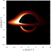Fig. 5 Intensity map of the thin disk model described in Sect. 3. Lensed images of up to tenth order are taken into account, where the order of an image is determined by the number of ray crossings of the equatorial plane. Higher-order images are ignored in the computation of the thin disk line spectra (Figs. 6a–d).

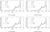Fig. 6 Redshift spectra of the thin disk model described in Sect. 3 for four different coordinate systems. The five different spin parameters examined in these plots are (in descending order for the peaked curves above Eobs ∕Eem = 1): − 0.99, −0.5, 0, 0.5, 0.99. The results may be compared with with Schnittman & Bertschinger (2004) and Dexter & Agol (2009).

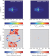Fig. 7 Intensity maps at 230 GHz for the comparison test, with a resolution of 4096 × 4096 pixels. The RAPTOR output (top left panel) and BHOSS output (top right panel) show excellent agreement in total flux density. The relative difference between the output of both codes is plotted in the bottom left panel. The deviations become quite large in the periphery of the image; since the intensity in these regions is low, however, they do not contribute significantly to the integrated flux density, as can be seen in the absolute difference between the two codes (bottom right panel).

4.2.2 Synchrotron images of accretion flow simulated with BHAC

As a final test for our radiative-transfer integrator, we performed a radiative-transfer simulation through GRMHD simulations of hot accretion flow onto a SMBH with properties matching those observed in Sagittarius A* (Sgr A*). The simulations are produced using the BHAC three-dimensional (3D) GRMHD code (Porth et al. 2017). During these calculations, the performance of RAPTOR is monitored.

The dominant emission mechanism of many low-frequency (radio and millimeter wavelengths) models of Sgr A* is continuum synchrotron emission from a relativistically hot magnetized plasma, that is, with Θ _e := k_BT_e∕m_ec² ≳ 1, with k_B, T_e, and m_e being the Boltzmann constant, the electron temperature and mass, respectively. The synchrotron emission and absorption coefficients depend on the electron distribution function. Here, and in the remaining part the paper, we assumed that the electrons have a thermal, relativistic (Maxwell-Jüttner) distribution function: $$n_{\text{e}}^{\text{TH}}(\gamma )=\frac{n_{\text{e}}^{\text{TH}}\gamma \sqrt{{\gamma }^2-1}\exp \left(-\gamma /{\Theta }_{\text{e}}\right)}{{\Theta }_{\text{e}}{K}_2\left(1/{\Theta }_{\text{e}}\right)},$$(41) where γ is an electron’s Lorentz factor and K₂ is the modified Bessel function of the second kind. The normalization constant $n_{\text{e}}^{\text{TH}}$ is the total electron number density, given by integrating the distribution function over all possible electron Lorentz factors: $n_{\text{e}}^{\text{TH}}={\displaystyle {\int }_1^{\infty }{n}_{\text{e}}^{\text{TH}}}\left(\gamma \right)\text{d}\gamma$.

The synchrotron emission coefficient j_ν of an ensemble of electrons is obtained by integrating the synchrotron emission coefficient of a single electron over the electron energies described by the above distribution function. Since the above expression contains a Bessel function, direct integration is time-consuming. In order to reduce the required computing time for radiative-transfer calculations,we used an approximate formula for the synchrotron emission coefficient provided by Leung et al. (2011): $$j_{\nu }^{\text{TH}}(\nu ,\theta )=\frac{\sqrt{2}\pi {\text{e}}^2{n}_{\text{e}}^{\text{TH}}{\nu }_s}{3c{K}_2({\Theta }_{\text{e}}^{-1})}{\left(X^{1/2}+2^{11/12}{X}^{1/6}\right)}^2\exp \left(-X^{1/3}\right)\text{},$$(42) where X is a dimensionless quantity given by $$X:=\frac{\nu }{{\nu }_{\text{s}}},$$(43) and ν_s is the critical frequency for the synchrotron emission: $${\nu }_{\text{s}}=\frac{2}{9}\left(\frac{eB}{2\pi m_{\text{e}}c}\right){\Theta }_{\text{e}}^2\sin \theta .$$(44)

Here, B is the magnetic field in the inertial frame, θ is the angle between the photon wave vector k^μ and the magnetic field four-vector b^μ in the fluid frame, and e is the unit electric charge. The angle θ is calculated by using Eq. 73 in Dexter (2016). Here, we used CGS units, so that the B field is given in (Gauss) and n_e is given in (cm ⁻³). The synchrotron emission coefficient therefore has units of (ergs s⁻¹ Hz⁻¹ cm⁻³). In this test, we assumed that $K_2\left({\Theta }_{\text{e}}^{-1}\right)=2{\Theta }_{\text{e}}^2$, which is an approximation. However, evaluating properly the Bessel function can yield differences in the integrated flux on the order of a few percent at most.

As shown in Leung et al. (2011), Eq. (42) is a good approximation of the true synchrotron emission coefficient for a range of electron temperatures Θ_e and frequencies ν. For θ = 30°, the relative error of the approximate emission coefficient formula is less than 1% for Θ _e > 0.5, and ν∕ν_c > 10 (where ν_c = eB∕2πm_ec = 2.8 × 10⁶B Hz is the electron cyclotron frequency). For θ = 80°, the error is less than 1% when Θ_e > 0.5 and ν∕ν_c > 10⁴. In our models, the typical magnetic field strength is B ≃ 10 Gauss, so ν_c ≃ 10⁷ Hz. Hence, when modeling the emission at frequencies around ν = 10¹¹ Hz, the approximate synchrotron emission coefficient formula given by Eq. (42) is very accurate.

The synchrotron self-absorption coefficient for a thermal distribution of electrons is derived from Kirchhoff’s law, ${\alpha }_{\nu }^{\text{TH}}=j_{\nu }^{\text{TH}}/B_{\nu }$, where ${\alpha }_{\nu }^{\text{TH}}$ is given in (cm⁻¹) and B_ν is the Planck function: $$B_{\nu }:=\frac{2h{\nu }^3}{c^2}\frac{1}{\exp \left(h\nu /(m_{\text{e}}{c}^2{\Theta }_{\text{e}})\right)-1}.$$(45)

BHAC (and similar GRMHD codes such as HARM) employ geometrized units, so that to carry out radiative-transfer calculations using the GRMHD simulation data for the plasma variables we must scale the GRMHD variables using the rest-mass density scaling factor ${\rho }_0:=\mathcal{M}/{\mathcal{L}}^3$ and the magnetic field strength scaling factor $B_0:=c\sqrt{4\pi {\rho }_0}$. Here, $\mathcal{L}=GM/c^2$ and $\mathcal{T}=GM/c^3$ are the simulation’s length and time scale factors, respectively; they are functions of the black hole’s mass only. The mass unit, $\mathcal{M}$, is a free parameter of the model. The electron number density used in the synchrotron emission/absorption coefficient formulae is then calculated using $$n_{\text{e}}=\rho \frac{{\rho }_0}{(m_{\text{e}}+m_{\text{p}})}{\text{cm}}^{-3}.$$(46)

In our GRMHD model, the temperature of protons T_p is proportional to the ratio of the plasma’s pressure and density, so that it is a scale-free quantity. The electron temperature T_e, which is essential to calculating the synchrotron emissivities, is parametrized by the proton-to-electron temperature ratio, which can be either constant or a function of GRMHD data variables. The key parameters for the test simulation are listed in Table 2, where τ_cutoff represents the optical depth at which integration is terminated (radiation emitted past this optical depth will have a negligible effect on theimage).

It is found that, when using 10 CPU cores, RAPTOR integrates 10 707 geodesics per second, while with one GPU unit, RAPTOR integrates 104 900 geodesics per second. The total run time for an image of 2000 × 2000 pixels was less than one minute using a GPU. A more detailed description of the code performance is given in Appendix B.

Figure 7 (top left panel) presents an image computed by RAPTOR of our GRMHD accretion flow simulation created in BHAC. We compared our results to images produced by another radiative transfer code, BHOSS (Younsi, in prep.; top right panel),which uses a different set of algorithms to RAPTOR. The total fluxes from both codes as a function of image resolution are given in Table 3. BHOSS and RAPTOR converge to almost identical total flux values, with a relative difference of 0.06% at a resolution of4096 × 4096 pixels. The percentage difference for every pixel in both images is presented in the bottom left panel, while the absolute difference between both images is shown in the bottom right panel. The overall structure of the images is consistent; the largest percentage differences are found in regions of low specific intensity, whose contribution to the observed flux density is negligible (see bottom right panel).

A possible source of the differences between BHOSS and RAPTOR is the fact that the two codes employ different approaches for computing step-sizes. BHOSS uses an algorithm that depends on the optical depth of the plasma, while RAPTOR bases its step-size purely on the geometry of spacetime. This results in different sampling strategies which, although not a dominant factor in the total flux, can nonetheless result in large deviations in a plot of the relative difference between the two images. Looking at the images and total fluxes, we conclude that the codes give consistent results while using different methods to solve the radiative transport and geodesic equations. The GRMHD file used in this comparison is included with the RAPTOR code.

5 Time-dependent radiative transfer in GRMHD simulations

GRMHD simulations dump their data in so-called snapshots – instantaneous states of the plasma captured at discrete moments during the simulation. When creating images based on a series of GRMHD snapshots using radiative-transfer calculations,it is either possible to ignore a geodesic’s time coordinate, thereby treating the GRMHD snapshot as static while the rays propagate (this is normally referred to as the fast-light approximation), or it is possible to keep track of the geodesic’s time coordinate, interpolating between different GRMHD snapshots so as to obtain the plasma conditions that are correct not only in space but also in time (this is normally referred to as the slow-light approximation).

In order to generate the results of this section, we relaxed the assumption of staticity of the GRMHD simulation during radiative-transfer calculations and thus implement the slow-light approximation with the goal of improving the accuracy of our model in predicting the properties of the accretion flow onto a SMBH. In such relativistic plasmas, the effects of selecting the fast-/slow-light approximation can be arbitrarily great or small based on the geometry and observer under consideration. For instance, Dexter et al. (2010) considered the differences between fast-light and slow-light in the context of a particular accreting black-hole model and concluded that the differences were minimal. Here, we return to this problem as new models with more complex electron thermodynamics have been developed. Overall, we are here interested in verifying the fast-light approximation in a broader context.

In GRMHD simulations such as those performed by HARM2D or BHAC, only the heavy ions are simulated. In radiative processes, however, ions are not the dominant source of emission, and we therefore need a description to couple the electrons in the plasma to their ionic counterparts. To do so, we implemented a one-fluid model in which the coupling between the two species changes throughout the simulation volume as a function of the β_p plasma parameter (Mościbrodzka et al. 2016) 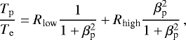$$\frac{T_{\text{p}}}{T_{\text{e}}}=R_{\text{low}}\frac{1}{1+{\beta }_{\text{p}}^2}+R_{\text{high}}\frac{{\beta }_{\text{p}}^2}{1+{\beta }_{\text{p}}^2},$$(47) where β_p := P_gas∕P_mag is the ratio of gas pressure to magnetic-field pressure P_mag = B²∕2, and R_low and R_high are two free parameters. In strongly magnetized plasmas, β_p ≪ 1 and T_p∕T_e → R_low. In weakly magnetized plasmas, on the other hand, β_p ≫ 1 and so T_p∕T_e → R_high.

The models used in this section are motivated by qualitatively reproducing the observed spectrum of Sgr A* (Shcherbakov et al. 2012). Our primary focus, however, is on investigating the difference (if any) between the fast-light and slow-light paradigms, rather than on reproducing the source in great detail. More precisely, the parameters assumed for our modeling are that the SMBH has a mass of M = 4 × 10⁶ M_⊙ and is at a distance of d = 7.88 × 10³ pc (Boehle et al. 2016), that the observer has an inclination of 60° and performs observationsat frequencies of 22, 43, 86, and 230 GHz.

5.1 Time calibration

When comparing slow and fast-light simulations it is important to describe how the results align when comparing them. The reason for this is that a single image from a slow-light calculation uses data from many GRMHD slices, so that it is no longer possible to associate an image with a specific GRMHD slice, as is possible in the case of a fast-light calculation. This also means that a large number of GRMHD slices are needed for slow-light calculations: the slices of GRMHD data should extend from the moment in time when the first ray enters the simulation volume until the moment when the last ray leaves it. When taking curvature into account, these moments are difficult to compute and depend on the initial conditions of the camera rays: some images can contain rays that pass close to the event horizon, circling the black hole many times before escaping (see Fig. 4), thus delaying their exit time, potentially indefinitely for pathological rays. We here neglected the contribution of these rays for two reasons; first, the optical depth along such a ray would cause virtually all emission beyond a certain value for the affine parameter to be absorbed; second, rays that orbit the black hole for a an increasing number of times are increasingly rare, thus contributing only marginally to our images.

In practice, we established the alignment by introducing an empirically determined time delay in our rays’ initial time coordinate in such a way that light curves from the fast-light and slow-light simulations at an inclination angle of 90° coincide; this is effectively equivalent to translating the slow-light light curve with respect to the fast-light light curve on the time axis.

5.2 Results

The model whose emission is dominated by the disk is characterized by a mass scale factor, $\mathcal{M}=5.03\times {10}^{-15}{M}_{\odot }$ and the weak-magnetization electron-proton temperature ratio R_high = R_low = 1. Slow-light images of the accretion disk at our 4 VLBI frequencies are presented in Fig. 8 (we do not report the corresponding fast-light images as they are virtually indistinguishable). Light curves for both the slow-light and fast-light simulations, along with residuals, are presented in Fig. 9, while normalized light curves at all frequencies for the slow-light simulation of the disk-emission model are shown in Fig. 10.

Similarly, the model whose emission is dominated by the jet is characterized by a mass scale factor $\mathcal{M}=2.515\times {10}^{-13}{M}_{\odot }$ and the weak-magnetization electron-proton temperature ratio R_high = 25 (while R_low = 1). In this case, slow-light images of the accretion flow at all VLBI frequencies are shown in Fig. 11, while the light curves of fast- and slow-light simulations are reported in Fig. 12; finally the normalized slow-light light curves at all frequencies are shown in Fig. 13.

We found that the difference between the fast-light and slow-light approaches is systematically below 5% in all cases, suggesting that the fast-light approximation is a good one for the model presently under consideration, a result that is in line with the findings of Dexter et al. (2010).

As a concluding remark, we note that we have considered radiative-transfer calculations of the unpolarized component of synchrotron radiation. This is motivated by the fact that observations show that linear and circular polarization of Sgr A* are less than a few percent (Bower et al. 2003). Although small, the polarization is nonzero and we here speculate that the differences between the two approaches may become more pronounced when considering the polarized components of the radiation.

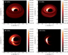Fig. 8 Images of our slow-light-simulation of the disk emission dominated model at VLBI frequencies. The flux density is given in units of Jy pixel−2.

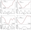Fig. 9 Light curves for slow-light (solid) and fast-light (dashed) for the disk emission dominated model at VLBI frequencies. Residuals are displayed below the light curves.

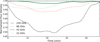Fig. 10 Normalized light curves of slow-light simulations at the VLBI frequencies (230 GHz (solid), 86 GHz (dashed), 43 GHz (solid and dotted), 22 GHz (dotted)) for viewing angle of 60 degrees for our disk dominated model.

Fig. 11 Images of our slow-light-simulation of the jet emission dominated model at VLBI frequencies. Flux density is given in units of Jy pixel−2.

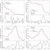Fig. 12 Light curves for slow-light (solid) and fast-light (dashed) for the jet emission dominated model at VLBI frequencies. Residuals are displayed below the light curves.

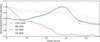Fig. 13 Normalized light curves of slow-light simulations at the VLBI frequencies (230 GHz (solid), 86 GHz (dashed), 43 GHz (solid and dotted), 22 GHz (dotted)) for viewing angle of 60° for our jet dominated model.

6 Summary

We have introduced RAPTOR, a new time-dependent radiative-transfer code capable of producing physically accurate images of black-hole accretion disks as calculated by GRMHD simulations in particular, and of performing radiative-transfer calculations in general astrophysical problems that involve radiative transfer and strong gravity in general. The code achieves this result by integrating null geodesics in arbitrary spacetimes and then performing time-dependent radiative transport along the geodesics to ultimately construct images, light curves, and spectra. Furthermore, RAPTOR is capable of time-dependent computations, in which the characteristics of a single image may depend on a range of input data in the time domain and it can be run on both CPUs and GPUs.

We have verified correctness of our geodesic calculations by investigating the conservation of constants of motion and comparing our results to the semi-analytical code geokerr, our results being in good agreement. The same procedure was applied to our radiative-transfer computations: we performed a number of tests of our various integration schemes and reproduced results from the literature.

As an additional verification step, we compared our code directly to the another recently developed radiative-transfer code: BHOSS (Younsi, in prep.). We considered a complex scenario that involves a particular set of GRMHD data along with a physical radiative model and produced images of the accretion flows using both codes. The result was a convergence of the total flux density as computed by the two codes, which rely on different integration algorithms for both null geodesics and radiative transfer, to a relative error of less than 0.01% (see Fig. 7), demonstrating that our implementations are highly consistent.

An important validation of our code has come from neglecting a commonly made assumption that the physical properties of the underlying plasma do not vary during the propagation of the radiation (fast-light approximation). We have therefore studied the difference between the slow-light and fast-light paradigms in radiative models of accretion flows onto SMBHs. The differences between slow-light and fast-light can be arbitrarily large or utterly negligible, depending on the physical conditions. In context we have considered, where we have investigated radiative models based on 2D GRMHD data, we conclude that the effects of switching between the fast-light and slow-light paradigms on the appearance of this particular model’s accretion flow are smaller than 5% across the VLBI frequencies we examined.

While these results are in agreement with the findings of Dexter et al. (2010) we note that this conclusion may be influenced by the fact that we have investigated unpolarized radiative transfer only. In conclusion, the RAPTOR code – and its further developments in terms of the possibility of treating polarized radiative transfer – may be used to compare synthetic images of SMBH accretion flows to mm-VLBI data from the Event Horizon Telescope Collaboration¹ and to extract physical properties of the black-hole system (e.g., spin, inclination) or to test the predictions of GR about the size and shape of the black-hole shadow. The code has many potential applications in other astrophysical problems, such as radiative transfer near a neutron star or a binary black-hole system. It is also well-suited to creating material for outreach purposes, such as virtual-reality movies of black hole environments (Davelaar et al., in prep.).

Finally, we note that because the electron distribution function of the plasma is an important factor in determining radiative properties, reducing the number of assumptions made about this function may have an appreciable effect on the synthetic observational data one may generate using our models. In view of this, we have recently added a more general particle distribution function than the one presented here, relaxing the assumption that the electrons are in a thermal distribution by adding accelerated particles and thereby improving the accuracy of radiative models. The results of this analysis will be presented in a distinct and forthcoming paper (Davelaar et al. 2018).

Acknowledgements

This work is supported by the ERC Synergy Grant “BlackHoleCam: Imaging the Event Horizon of Black Holes” (Grant 610058). Z.Y. acknowledges support from an Alexander von Humboldt Fellowship. This research has made use of NASA’s Astrophysics Data System. Some of the simulations in this work were performed on the LOEWE cluster in CSC in Frankfurt.

Appendix A: Coordinate Transformations

Here, we listcertain non-trivial coordinate transformations that are used in RAPTOR. In what follows, the BL coordinates are denoted by (t, r, θ, ϕ), and the KS coordinates by $(\tilde{t},r,\theta ,\tilde{\varphi })$.

A.1:

BL-KS

The transformations of the coordinate vector between BL and KS coordinates is given by (see e.g., Font et al. 1999): 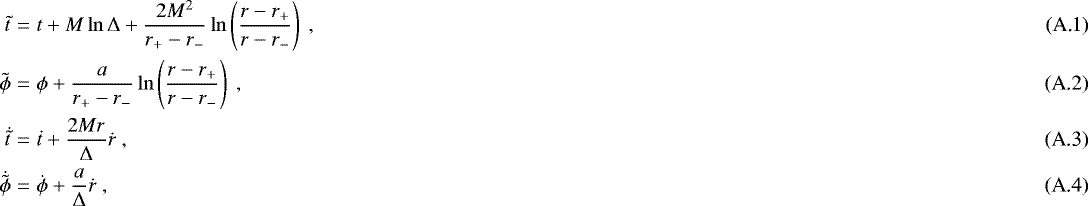$$\begin{array}{lll}\tilde{t}\hfill & =\hfill & t+M\ln \Delta +\frac{2M^2}{r_{+}-r_{-}}\ln \left(\frac{r-r_{+}}{r-r_{-}}\right),\hfill \\ \tilde{\varphi }\hfill & =\hfill & \varphi +\frac{a}{r_{+}-r_{-}}\ln \left(\frac{r-r_{+}}{r-r_{-}}\right),\hfill \\ \dot{\tilde{t}}\hfill & =\hfill & \dot{t}+\frac{2Mr}{\Delta }\dot{r},\hfill \\ \dot{\tilde{\varphi }}\hfill & =\hfill & \dot{\varphi }+\frac{a}{\Delta }\dot{r},\hfill \end{array}$$ where an overdot denotes differentiation with respect to the affine parameter, λ, 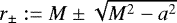$r_{\pm }:=M\pm \sqrt{M^2-a^2}$ denotes the outer(inner) event horizon radius, Δ = r² − 2Mr + a² := (r − r₊)(r − r₋) and M is the black-hole mass. It is important to note that these transformations are valid only in the region of spacetime exterior to the black-hole horizon.

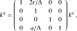
Four-vectors transform differently. In RAPTOR, the initial contravariant wave vector $k_0^{\mu }$ is always constructed using BL coordinates, and must be transformed to KS coordinates. This is accompanied by the following transformation matrix (McKinney & Gammie 2004): $$k^{\overline{\alpha }}=\left(\begin{array}{cccc}1& 2r/\Delta & 0& 0\\ 0& 1& 0& 0\\ 0& 0& 1& 0\\ 0& a/\Delta & 0& 1\end{array}\right)k^{\alpha },$$(A.5) where k^α denotes the wave vector in BLcoordinates, $k^{\overline{\alpha }}$ is the wave vector in KS coordinates. The reverse transformation is given by $$k^{\alpha }=\left(\begin{array}{cccc}1& -2r/\Delta & 0& 0\\ 0& 1& 0& 0\\ 0& 0& 1& 0\\ 0& -a/\Delta & 0& 1\end{array}\right)k^{\overline{\alpha }}.$$(A.6)

A.2:

KS-MKS

The modified Kerr-Schild coordinates (MKS), as used by, for example, Gammie et al. (2003), are denoted by $(\tilde{t},x^1,x^2,\tilde{\varphi })$. Some of these quantities may be expressed in terms of conventional KS coordinates as: $$\begin{array}{lll}{x}^1\hfill & =\hfill & \ln \left(r-r_0\right),\hfill \\ {\dot{x}}^1\hfill & =\hfill & \frac{\dot{r}}{r-r_0},\hfill \\ {\dot{x}}^2\hfill & =\hfill & \frac{\dot{\theta }}{\pi \left[1+\left(1-h\right)\cos \left(2\pi x^2\right)\right]},\hfill \end{array}$$ where 0 ≤ h ≤ 1 is obtained from the GRMHD data and stretches the zenith coordinate near the poles and the equatorial plane. Notice that we cannot obtain x²(θ) algebraically as this requires solving a transcendental equation; we must find it numerically, via the inverse transformation x² → θ, which can be written in closed form. This transformation, along with the corresponding inverse transformations for Eqs. (A.7), (A.8), and (A.9), may be written as: $$\begin{array}{lll}r\hfill & =\hfill & r_0+\exp x^1,\hfill \\ \theta \hfill & =\hfill & \pi x^2+\frac{1}{2}\left(1-h\right)\sin \left(2\pi x^2\right)\text{},\hfill \\ \dot{r}\hfill & =\hfill & {\dot{x}}^1\left(r-r_0\right)\text{},\hfill \\ \dot{\theta }\hfill & =\hfill & \pi {\dot{x}}^2\left[1+\left(1-h\right)\cos \left(2\pi x^2\right)\right]\text{}.\hfill \end{array}$$

To perform the transformation θ → x², we must resort to numerically (indeed iteratively) seeking a value x² that satisfies Eq. (A.11), and this is readily performed using the Newton-Raphson method. For a function f(x) the solution to f(x) = 0 may be found iteratively as: $$x_{n+1}=x_n-\frac{f(x_n)}{f^{\prime }(x_n)},$$(A.14) where f′(x_n) := df(x_n)∕dx_n and the index n denotes the iterative step. For MKS coordinates we have: $$\begin{array}{lll}f(x_n^2)\hfill & =\hfill & \left[\pi x_n^2+\frac{1}{2}\left(1-h\right)\sin \left(2\pi x_n^2\right)-\theta \right],\hfill \\ f^{\prime }(x_n^2)\hfill & =\hfill & \pi \left[1+\left(1-h\right)\cos \left(2\pi x_n^2\right)\right],\hfill \end{array}$$ since $\partial \theta /\partial x_n^2=0$ and θ is constant in the above iterative scheme. One must start with a trial value for $x_0^2\ll 1$ and then iterate from there. Since x² ∈ [0, 1], if $x_{n+1}^2<0$ or $x_{n+1}^2>1$ then reset $x_{n+1}^2$ to a small value (e.g., 0.05). We also apply the above reset if $f^{\prime }(x_n^2)\to 0$. Finally, we define a appropriate convergence criterion, namely $|x_{n+1}^2-x_n^2|<\epsilon$, where ε is the error tolerance we find acceptable.

Appendix B: Code performance

As mentioned in the Introduction, an important added value of RAPTOR is that it is a hybrid code that can be compiled for both CPUs and GPUs. Two distinct parallelization methods are implemented in the code; one is OpenMP², with which it is possible to run the code on multiple CPU cores; the other is OpenACC, with which it is possible to run the code on both the CPU and GPU. We have verified and tested the performance of the code in these environments by considering a radiative-transfer calculation through our BHAC GRMHD simulation. The model parameters are listed in Table B.1. More specifically, we investigate how the performance of RAPTOR scales with the number of threads that are employed. This is done by running the same setup (Table B.1) on the same hardware (Table B.2) multiple times, using a different number of cores each time.

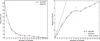Fig. B.1 Run time (left) and speed-up factor (right) for RAPTOR using OpenMP and OpenACC.

The scalability is measured by calculating the speed-up factor, which is defined as $$\text{S}=T_{\#\text{threads}}/T_{\text{single\hspace{0.17em}thread}},$$(B.1) where T is the run time of the code for a given amount of threads.

The results of our runs can be found in Fig. B.1 and they show that the code scales sub-linearly with the number of cores, as is expected, since communication overhead increases with an increasing number of threads; again, as expected, the GPU runs outperform the CPU ones. Interestingly, the OpenMP implementation slightly outperforms OpenACC, but this is not surprising, since OpenACC lacks hyper-threading support for CPUs, which is instead provided with OpenMP. When using 10 CPU-cores, RAPTOR can integrate 10 707 geodesics per second, while with one GPU unit, RAPTOR integrates 104 900 geodesics per second.

One reason why the difference between GPU and CPU performance is relatively small is the additional time required for data transfer andkernel booting operations in the GPU based implementation. We therefore also rendered a large image (2000 × 2000 pixels) on both the CPU and GPU, to check whether the difference between CPU and GPU performance increases. The average run times are 3 minutes and 58 seconds on one CPU, and 39 seconds on one GPU, respectively. As expected, the difference in performanceis substantially increased under these conditions.

These total run times also include data read (~1 s) and output generation (~0.2 s) operations. Overall, the calculation of the image on the GPU took 2.5 s.

References

All Tables

All Figures

Fig. 1 Radiative-transfer variables along a particular null geodesic that intersects a radiating plasma near a Kerr black hole (see Fig. 2). Top: local specific intensity Iν (dashed red curve), which is computed by integrating Eq. (34) in the direction of increasing affine parameter λ, and of the specific intensity seen by the observer, Iν,obs (solid black curve), which is computed by integrating Eq. (37) in the direction of decreasing λ. The intensity is normalized with respect to the observed intensity in both cases, so that we expect both curves to approach unity with continued integration, which is illustrated using the blue guideline. We note that Iν is a non-monotonic function of λ while Iν,obs is a monotonic function of λ. We also notethat for Iν,obs and τν,obs, integration proceeds from right to left in these plots, and that Iν,obs converges much faster than Iν. Bottom: optical depth for the same ray.

In the text

Fig. 2 Synchrotron emission map created using a GRMHD simulation (see Sect. 4.2.2) made using the HARM code (Gammie et al. 2003). Intensity is given in units of Jy pixel−2. The observer frequency is 100 GHz, the inclination angle is 30 degrees, and the disk-dominated emission model discussed in Sect. 5 is used. Note the optically-thick accretion disk and strong emission to the left of the black-hole shadow (this region appears bright due to relativistic beaming). The ray investigated in Fig. 1 is marked by a white dot in this image. This particular ray, travelling from the plasma to the observer, first passes through the bright, relativistically-boosted region, and then through an optically-thick, non-boosted region of the disk, suggesting that the specific intensity along this ray will sharply increase, then decrease, before reaching the observer. Figure 1 shows that this is indeed the case.

In the text

Fig. 3 Convergence plots for the L1-error norms of the conserved quantities E (dashed blue), L (solid black), and Q (dotted red) for the orbit with parameters i = 90°, α = −3.22, β = 1.12, a = 0.998 with different integrator settings. The errors are computed at a fixed coordinate time tfinal. Two guide lines with slopes −2 (solid) and −4 (dashed) are drawn. The +, −, and ×-symbols represent respectively L, Q, and E, for the RK4integrator. The square, hexagon, and circle symbols represent the same quantities for the Verlet integrator.

In the text

Fig. 4 Comparison of null geodesics computed by the semi-analytical integrator geokerr to those computed by our fully numerical code. In each case, the geodesic represented by the black dots was computed using geokerr while the geodesic represented by the white dotted line is the output of RAPTOR (dots were chosen for the former geodesic because its variable step-size can otherwise create interpolation issues). The gray spheroid represents the black hole’s outer event horizon. MKS coordinates were used with ϵ = 0.001. The parameters for these geodesics are listed in Table 1.

In the text

	Fig. 5 Intensity map of the thin disk model described in Sect. 3. Lensed images of up to tenth order are taken into account, where the order of an image is determined by the number of ray crossings of the equatorial plane. Higher-order images are ignored in the computation of the thin disk line spectra (Figs. 6a–d).
In the text

	Fig. 6 Redshift spectra of the thin disk model described in Sect. 3 for four different coordinate systems. The five different spin parameters examined in these plots are (in descending order for the peaked curves above Eobs ∕Eem = 1): − 0.99, −0.5, 0, 0.5, 0.99. The results may be compared with with Schnittman & Bertschinger (2004) and Dexter & Agol (2009).
In the text

Fig. 7 Intensity maps at 230 GHz for the comparison test, with a resolution of 4096 × 4096 pixels. The RAPTOR output (top left panel) and BHOSS output (top right panel) show excellent agreement in total flux density. The relative difference between the output of both codes is plotted in the bottom left panel. The deviations become quite large in the periphery of the image; since the intensity in these regions is low, however, they do not contribute significantly to the integrated flux density, as can be seen in the absolute difference between the two codes (bottom right panel).

In the text

	Fig. 8 Images of our slow-light-simulation of the disk emission dominated model at VLBI frequencies. The flux density is given in units of Jy pixel−2.
In the text

	Fig. 9 Light curves for slow-light (solid) and fast-light (dashed) for the disk emission dominated model at VLBI frequencies. Residuals are displayed below the light curves.
In the text

	Fig. 10 Normalized light curves of slow-light simulations at the VLBI frequencies (230 GHz (solid), 86 GHz (dashed), 43 GHz (solid and dotted), 22 GHz (dotted)) for viewing angle of 60 degrees for our disk dominated model.
In the text

	Fig. 11 Images of our slow-light-simulation of the jet emission dominated model at VLBI frequencies. Flux density is given in units of Jy pixel−2.
In the text

	Fig. 12 Light curves for slow-light (solid) and fast-light (dashed) for the jet emission dominated model at VLBI frequencies. Residuals are displayed below the light curves.
In the text

	Fig. 13 Normalized light curves of slow-light simulations at the VLBI frequencies (230 GHz (solid), 86 GHz (dashed), 43 GHz (solid and dotted), 22 GHz (dotted)) for viewing angle of 60° for our jet dominated model.
In the text

	Fig. B.1 Run time (left) and speed-up factor (right) for RAPTOR using OpenMP and OpenACC.
In the text

References

- Abbott, B. P., Abbott, R., Abbott, T. D., et al. 2016, Phys. Rev. Lett., 116, 061102 [Google Scholar]
- Bardeen, J. M., Press, W. H., & Teukolsky, S. A. 1972, ApJ, 178, 347 [NASA ADS] [CrossRef] [Google Scholar]
- Beloborodov, A. M. 2002, ApJ, 566, L85 [NASA ADS] [CrossRef] [Google Scholar]
- Boehle, A., Ghez, A. M., Schödel, R., et al. 2016, ApJ, 830, 17 [NASA ADS] [CrossRef] [Google Scholar]
- Bower, G. C., Wright, M. C. H., Falcke, H., & Backer, D. C. 2003, ApJ, 588, 331 [NASA ADS] [CrossRef] [Google Scholar]
- Boyer, R. H., & Lindquist, R. W. 1967, J. Math. Phys., 8, 265 [NASA ADS] [CrossRef] [Google Scholar]
- Broderick, A. E. 2006, MNRAS, 366, L10 [NASA ADS] [CrossRef] [Google Scholar]
- Carter, B. 1968, Phys. Rev., 174, 1559 [NASA ADS] [CrossRef] [Google Scholar]
- Chan, C.-k., Psaltis, D., & Özel, F. 2013, ApJ, 777, 13 [NASA ADS] [CrossRef] [Google Scholar]
- Chan, C.-k., Medeiros, L., Ozel, F., & Psaltis, D. 2017, ApJ, submitted, [arXiv:1706.07062] [Google Scholar]
- Chirenti, C. & Rezzolla, L. 2016, Phys. Rev. D, 94, 084016 [NASA ADS] [CrossRef] [Google Scholar]
- Cunningham, C. T. & Bardeen, J. M. 1972, ApJ, 173, L137 [NASA ADS] [CrossRef] [Google Scholar]
- Davelaar, J., Moscibrodzka, M., Bronzwaer, T., & Falcke, H. 2018, A&A, 612, A34 [NASA ADS] [CrossRef] [EDP Sciences] [Google Scholar]
- De Falco, V., Falanga, M., & Stella, L. 2016, A&A, 595, A38 [NASA ADS] [CrossRef] [EDP Sciences] [Google Scholar]
- Dexter, J. 2016, MNRAS, 462, 115 [NASA ADS] [CrossRef] [Google Scholar]
- Dexter, J., & Agol, E. 2009, ApJ, 696, 1616 [NASA ADS] [CrossRef] [Google Scholar]
- Dexter, J., Agol, E., Fragile, P. C., & McKinney, J. C. 2010, ApJ, 717, 1092 [NASA ADS] [CrossRef] [Google Scholar]
- Doeleman, S. S., Weintroub, J., Rogers, A. E. E., et al. 2008, Nature, 455, 78 [NASA ADS] [CrossRef] [PubMed] [Google Scholar]
- Doeleman, S. S., Fish, V. L., Schenck, D. E., et al. 2012, Science, 338, 355 [NASA ADS] [CrossRef] [PubMed] [Google Scholar]
- Dolence, J. C., Gammie, C. F., Mościbrodzka, M., & Leung, P. K. 2009, ApJS, 184, 387 [NASA ADS] [CrossRef] [Google Scholar]
- Falcke, H., & Markoff, S. B. 2013, Class. Quant. Grav., 30, 244003 [Google Scholar]
- Falcke, H., Melia, F., & Agol, E. 2000, ApJ, 528, L13 [NASA ADS] [CrossRef] [PubMed] [Google Scholar]
- Fish, V., Akiyama, K., Bouman, K., et al. 2016, Galaxies, 4, 54 [NASA ADS] [CrossRef] [Google Scholar]
- Font, J. A., Ibáñez, J. M., & Papadopoulos, P. 1999, MNRAS, 305, 920 [NASA ADS] [CrossRef] [Google Scholar]
- Gammie, C. F., McKinney, J. C., & Tóth, G. 2003, ApJ, 589, 444 [Google Scholar]
- Genzel, R., Eisenhauer, F., & Gillessen, S. 2010, Rev. Mod. Phys., 82, 3121 [NASA ADS] [CrossRef] [Google Scholar]
- Ghez, A. M., Salim, S., Weinberg, N. N., et al. 2008, ApJ, 689, 1044 [NASA ADS] [CrossRef] [Google Scholar]
- Goddi, C., Falcke, H., Kramer, M., et al. 2017, Int. J. Mod. Phys. D, 26, 02 [Google Scholar]
- Johnson, M. D., Fish, V. L., Doeleman, S. S., et al. 2015, Science, 350, 1242 [NASA ADS] [CrossRef] [Google Scholar]
- Kerr, R. P., & Schild, A. 1965, In IV Centenario Della Nascita di Galileo Galilei, A new class of vacuum solutions of the Einstein field equations, 1564 222 [NASA ADS] [Google Scholar]
- Konoplya, R., Rezzolla, L., & Zhidenko, A. 2016, Phys. Rev. D, 93, 064015 [NASA ADS] [CrossRef] [Google Scholar]
- Laor, A. 1991, ApJ, 376, 90 [NASA ADS] [CrossRef] [Google Scholar]
- Leung, P. K., Gammie, C. F., & Noble, S. C. 2011, ApJ, 737, 21 [NASA ADS] [CrossRef] [Google Scholar]
- Lindquist, R. W. 1966, Ann. Phys., 37, 487 [NASA ADS] [CrossRef] [Google Scholar]
- Luminet, J.-P. 1979, A&A, 75, 228 [NASA ADS] [Google Scholar]
- McKinney, J. C., & Gammie, C. F. 2004, ApJ, 611, 977 [NASA ADS] [CrossRef] [Google Scholar]
- Moscibrodzka, M., & Gammie, C. F. 2018, MNRAS, 475, 43 [NASA ADS] [CrossRef] [Google Scholar]
- Mościbrodzka, M., Gammie, C. F., Dolence, J. C., Shiokawa, H., & Leung, P. K. 2009, ApJ, 706, 497 [NASA ADS] [CrossRef] [Google Scholar]
- Mościbrodzka, M., Falcke, H., & Shiokawa, H. 2016, A&A, 586, A38 [NASA ADS] [CrossRef] [EDP Sciences] [Google Scholar]
- Noble, S. C., Leung, P. K., Gammie, C. F., & Book, L. G. 2007, Class. Quant. Grav., 24, 259 [Google Scholar]
- Novikov, I. D., & Thorne, K. S. 1973, In Astrophysics of black holes, eds. Dewitt, B. S., & Dewitt, C., Black Holes (Les Astres Occlus), 343 [Google Scholar]
- Parfrey, K., & Tchekhovskoy, A. 2017, ApJ, 851, L34 [NASA ADS] [CrossRef] [Google Scholar]
- Porth, O., Olivares, H., Mizuno, Y., et al. 2017, Comput. Astrophys. Cosmol., 4, 1 [Google Scholar]
- Poutanen, J., & Beloborodov, A. M. 2006, MNRAS, 373, 836 [NASA ADS] [CrossRef] [Google Scholar]
- Rezzolla, L., & Zhidenko, A. 2014, Phys. Rev. D, 90, 084009 [NASA ADS] [CrossRef] [MathSciNet] [Google Scholar]
- Schnittman, J. D., & Bertschinger, E. 2004, ApJ, 606, 1098 [NASA ADS] [CrossRef] [Google Scholar]
- Schnittman, J. D., & Rezzolla, L. 2006, ApJ, 637, L113 [NASA ADS] [CrossRef] [Google Scholar]
- Shcherbakov, R. V., & Huang, L. 2011, MNRAS, 410, 1052 [NASA ADS] [CrossRef] [Google Scholar]
- Shcherbakov, R. V., Penna, R. F., & McKinney, J. C. 2012, ApJ, 755, 133 [NASA ADS] [CrossRef] [Google Scholar]
- Swope, W. C., Andersen, H. C., Berens, P. H., & Wilson, K. R. 1982, J. Chem. Phys., 76, 637 [NASA ADS] [CrossRef] [Google Scholar]
- Takahashi, R., & Umemura, M. 2017, MNRAS, 464, 4567 [NASA ADS] [CrossRef] [Google Scholar]
- Viergutz, S. U. 1993, A&A, 272, 355 [NASA ADS] [Google Scholar]
- Younsi, Z., Wu, K., & Fuerst, S. V. 2012, A&A, 545, A13 [NASA ADS] [CrossRef] [EDP Sciences] [Google Scholar]
- Younsi, Z., Zhidenko, A., Rezzolla, L., Konoplya, R., & Mizuno, Y. 2016, Phys. Rev. D, 94, 084025 [NASA ADS] [CrossRef] [Google Scholar]