| Issue |
A&A
Volume 689, September 2024
|
|
|---|---|---|
| Article Number | A197 | |
| Number of page(s) | 14 | |
| Section | Astrophysical processes | |
| DOI | https://doi.org/10.1051/0004-6361/202348489 | |
| Published online | 13 September 2024 | |
Testing the existence of event horizons against rotating reflecting surfaces
1
Department of Astrophysics/IMAPP, Radboud University Nijmegen, PO Box 9010
6500 GL
Nijmegen, The Netherlands
2
Center for Astrophysics | Harvard & Smithsonian, 60 Garden Street, Cambridge, MA, 02138
USA
3
Black Hole Initiative at Harvard University, 20 Garden Street, Cambridge, MA, 02138
USA
4
Tsung-Dao Lee Institute, Shanghai Jiao Tong University, 520 Shengrong Road, Shanghai, 201210
PR China
5
School of Physics and Astronomy, Shanghai Jiao Tong University, 800 Dongchuan Road, Shanghai, 200240
PR China
6
Institut für Theoretische Physik, Goethe Universität, Max-von-Laue-Str. 1, 60438
Frankfurt, Germany
7
Anton Pannekoek Institute for Astronomy, University of Amsterdam, Science Park 904, 1098 XH
Amsterdam, The Netherlands
8
Departamento de Matemática da Universidade de Aveiro and Centre for Research and Development in Mathematics and Applications (CIDMA), Campus de Santiago, 3810-193
Aveiro, Portugal
Received:
4
November
2023
Accepted:
2
July
2024
Abstract
Context. Recently the Event Horizon Telescope observed black holes at event horizon scales for the first time, enabling us to now test the existence of event horizons.
Aims. Although event horizons have by definition no observable features, one can look for their non-existence. In that case, it is likely that there is some kind of surface, which like any other surface could absorb (and thermally emit) and/or reflect radiation. In this paper, we study the potential observable features of such rotating reflecting surfaces.
Methods. We construct a general description of reflecting surfaces in arbitrary spacetimes. This is used to define specific models for static and rotating reflecting surfaces, of which we study the corresponding light paths and synthetic images. This is done by numerical integration of the geodesic equation and by the use of the general relativistic radiative transfer code RAPTOR.
Results. The reflecting surface creates an infinite set of ring-like features in synthetic images inside the photon ring. There is a central ring in the middle and higher order rings subsequently lie exterior to each other converging to the photon ring. The shape and size of the ring features change only slightly with the radius of the surface R, spin a and inclination i, resulting in all cases in features inside the ‘shadow region’.
Conclusions. We conclude that rotating reflecting surfaces have clear observable features and that the Event Horizon Telescope might be able to observe the difference between reflecting surfaces and an event horizon for high reflectivities. Such reflecting surface models seem unlikely, which would strengthen the case that the black hole shadow indeed indicates the existence of an event horizon.
Key words: accretion / accretion disks / black hole physics / gravitation / radiative transfer / relativistic processes
Corresponding author; This email address is being protected from spambots. You need JavaScript enabled to view it. .
© The Authors 2024
 Open Access article, published by EDP Sciences, under the terms of the Creative Commons Attribution License (https://creativecommons.org/licenses/by/4.0), which permits unrestricted use, distribution, and reproduction in any medium, provided the original work is properly cited.
This article is published in open access under the Subscribe to Open model. This email address is being protected from spambots. You need JavaScript enabled to view it. to support open access publication.
1. Introduction
Black holes are a profound prediction of the theory of general relativity (GR; Einstein 1915). Although initially seen as purely theoretical objects occurring in highly symmetrical spacetimes (Schwarzschild 1916), the idea was taken more seriously after the discovery that they can be a natural result of gravitational collapse (Oppenheimer & Snyder 1939; Penrose 1965). Because of their compactness, deep potential well and possibilities for energy extraction (Penrose & Floyd 1971; Blandford & Znajek 1977), they became the best candidates for many high energy compact objects in astronomy. It was found that X-ray binaries contain stellar-mass black holes (Bolton 1972; Webster & Murdin 1972; McClintock & Remillard 1986) and that quasars are extremely luminous compact objects best explained by being supermassive black holes (SMBH; Schmidt 1963; Lynden-Bell 1969). It now seems that every galaxy contains a dark compact object at its center (Richstone et al. 1998) and that they may be important for the evolution of their host galaxy (Magorrian et al. 1998; Fabian 2012; Kormendy & Ho 2013). Recently, it has even become possible to do precision tests of gravity around black holes with the detection of gravitational waves with LIGO/VIRGO (Abbott et al. 2016, 2021), observations of the relativistic orbits of stars around Sagittarius A* (Sgr A*) using GRAVITY (GRAVITY Collaboration 2018, 2020; Do et al. 2019) and horizon scale images of Messier 87* (M 87*) and Sgr A* using very long baseline interferometry (VLBI) observations by the Event Horizon Telescope (EHT; Event Horizon Telescope Collaboration 2019a, 2022a).
The horizon scale images create a unique way to test gravity (Psaltis & Johannsen 2011; Psaltis et al. 2016; Goddi et al. 2017; Cunha & Herdeiro 2018; Psaltis 2019). The most prominent gravitational effect featured in the images is the black hole shadow (Falcke et al. 2000). It is the region in the image plane bounded by the impact parameters that when traced backward converge to tangent circular orbits (Cunningham & Bardeen 1973; Luminet 1979). This is a geometric feature independent of astrophysical effects. In observational images, it shows up as a central brightness depression (CBD). This is produced by the fact that light paths of impact parameters inside the shadow trace backward to the event horizon, therefore having small optical depths compared to impact parameters outside the shadow region (Jaroszynski & Kurpiewski 1997; Johannsen & Psaltis 2010; Narayan et al. 2019; Ozel et al. 2021; Bronzwaer & Falcke 2021; Kocherlakota & Rezzolla 2022). The radius of the shadow is proportional to the black hole mass and its shape can in some cases give information about the black hole spin, see for example (Younsi et al. 2016; van der Gucht et al. 2020).
The accretion around these low luminosity active galactic nuclei is described by the radiatively inefficient advection-dominated flows (Narayan et al. 1998a) and radio jets (Falcke & Biermann 1999; Nagar et al. 2001), which are both geometrically thick and optically thin at the observing frequency of 230 GHz. Accurate predictions of the visual appearance of black holes can be made using general relativistic magnetohydrodynamics (GRMHD) models to derive the dynamics of the surrounding plasma and magnetic fields, and general relativistic radiative transfer (GRRT) models to calculate the emission and radiative transfer through curved spacetime. The resulting synthetic images can be compared with observational images of M 87* and Sgr A*. This shows that the current observations are in agreement with the sources being Kerr black holes (Event Horizon Telescope Collaboration 2019b,c, 2022b,c).
Despite all this, there remain some fundamental unresolved questions concerning black holes. For one, the Penrose singularity theorem states that in the process of gravitational collapse curvature singularities are formed. The question is whether these are covered by an event horizon (as conjectured by the cosmic censorship conjecture Penrose 1969) or whether they are ‘naked’, that is observable. It is thought that quantum theory could prevent these curvature singularities; however, the combination of quantum theory and event horizons leads to the black hole information paradox (Hawking 1975) and other related problems (Harlow 2016). This is connected to the prediction in GR called the no-hair theorem that all stationary black hole spacetimes are characterized by only three externally observable classical quantities, namely the mass, charge and angular momentum (Kerr 1963; Israel 1967, 1968; Carter 1968, 1971; Hawking 1972; Price 1972a,b; Robinson 1975). In the case of overall charge neutrality, black holes thus should be described by the Kerr metric. A deviation of the Kerr metric together with an observation of an event horizon would then constitute a violation of the no-hair theorem and in extension a violation of GR.
Since the Event Horizon Telescope recently demonstrated the ability to observe black holes at event horizon scales, it has now become possible to look for signs of the existence of event horizons. By definition, event horizons have no direct observational features. To some degree, black hole shadows are their observational feature; however, they could be mimicked by other objects. We can look for the observational signs of these latter objects (Olivares et al. 2020) to indicate the possible non-existence of event horizons. If these objects create observational features inside the ‘shadow region’, then that would create a way to distinguish between them and event horizons. If that is the case for some or maybe all such alternatives to event horizons, then that would strengthen the position of black hole shadows as an indicator of the existence of an event horizon.
There are many proposed models for these exotic compact objects (Cardoso & Pani 2019). For them to have a shadow, they need to have some sort of light capture cross section. The compactness of these objects can be characterized by the distance of some would-be horizon ϵ. According to Buchdahl’s theorem (Buchdahl 1959), the compactness is bounded under certain conditions. Exotic objects smaller than this bound can be classified by which of these assumptions they violate, such as isotropy for anisotropic stars (Andréasson 2008). Examples of exotic compact objects possessing some kind of surface are gravastars (Mazur & Mottola 2004), anisotropic stars, and some boson stars where the bosonic fields interact with photons and other standard model particles. Some examples of alternatives would be naked singularities, wormholes and boson stars with no/weak interaction with photons.
In the case of a surface, the surface could absorb and/or reflect radiation like any other surface. In the case of absorption, the energy should be thermalized and reradiated as thermal emission. This argument is well developed (Narayan et al. 1998b; Narayan 2002; Broderick & Narayan 2006, 2007; Narayan & McClintock 2008; Broderick et al. 2009) and has been used to study M 87* and Sgr A* using the EHT images (Event Horizon Telescope Collaboration 2019c, 2022c). Vincent et al. (2021) looked at synthetic images of these ultracompact stars with an emitting surface.
Reflecting surfaces have been looked at first in the context of gravitational waves in the form of gravitational wave echoes (Cardoso et al. 2016a,b; Cardoso & Pani 2017). In the context of black hole imaging, the argument has only recently been introduced in Event Horizon Telescope Collaboration (2022c) and used to study Sgr A*. They looked at a static spherical surface near where the horizon would be in the Schwarzschild metric. Two assumptions were made: (i) any inward-moving wave vector  becomes an outward-moving wave vector
  with the radial component kr reversed and all other components unchanged:
 (1)
(1)
and (ii) if the intensity of an ingoing ray is Iν, then the intensity of the reflected ray is AIν, where A ≤ 1 is the albedo of the surface. The resulting synthetic images found using such a model contain two new features: a bright central ring and a ring exterior to that both inside the ‘shadow region’. For an albedo of A = 1, an image with a blur of 15 μas was clearly distinguishable from the image of the EHT and the particular model could be excluded. For lower albedos, the sensitivity is still too low to draw conclusions. This model has been studied further in Carballo-Rubio et al. (2022).
The reflection argument is new and can still be improved upon in many ways. For one, the model does not take rotation into account, despite the fact that the observations indicate the central object having a non-zero spin (Event Horizon Telescope Collaboration 2022b). In this paper, we generalize the model to rotating reflecting surfaces and study the potential observable features of such rotating reflecting surfaces.
The paper is structured as follows. In Sect. 2, the mathematical model of reflecting surfaces is described. First, a general model for subsequently static surfaces, moving surfaces in flat spacetime and surfaces in arbitrary spacetimes are discussed and developed. Then, specific models for static spherical surfaces and rotating surfaces are derived. In Sects. 3 and 4, respectively the resulting light paths and synthetic images in these models are explored. In Sect. 5, the results are discussed and Sect. 6 is the conclusion.
2. Models of reflecting surfaces
2.1. Types of reflection
When electromagnetic radiation reaches a boundary between two media, it can be transmitted, absorbed, and/or reflected. The relative amount of incoming radiation that is reflected is given by the albedo A, where A = 0 means that all is transmitted and/or absorbed and A = 1 that all is reflected. Depending on the particular interface, the reflection can be specular, diffuse or a combination of the two. Specular reflection is the mirror-like type of reflection, of which the properties in the case of a plane wave reflecting off a stationary planar surface can easily be derived from the Maxwell equations (Jackson 1999). In that case, the incident and reflected wave vectors form a plane called the plane of incidence, which contains the normal to the surface as well. The angles of the incident and reflected wave vectors with the normal are respectively the angle of incidence ∠i and the angle of reflection ∠f. These obey the law of reflection:
 (2)
(2)
In addition to that, the frequency and the intensity (up to a factor of the albedo A) are conserved.
Diffuse reflection is the type of reflection as seen for example from matte surfaces, where the incoming light is scattered in many different outgoing directions. We will see that given a model of diffuse reflection of a stationary surface, it is straightforward to adjust the reflection law to one describing diffuse reflection. However, the fact that instead of one, there is a continuum of resulting reflected wave vectors, makes it more difficult to do actual calculations with it. Therefore, we will restrict our attention in this paper to specular reflection.
2.2. Reflection off a moving surface in flat spacetime
The reflection of light off a uniformly moving surface was first described by Einstein in his 1905 paper introducing the theory of special relativity (Einstein 1905). Using a Lorentz transformation he transformed the intensity, angle and frequency of incident light to the frame of the surface. There he used the known reflection behavior for a stationary surface as described above. Finally, he transformed the reflected quantities back to the observer frame using the inverse Lorentz transformation. The surprising result obtained was that the angles of incidence and reflection no longer have to be equal, contrary to Eq. (2). The same is true for the incident and reflected intensity and frequency. All three quantities now depend on the velocity and orientation of the surface. This result has since then been well established, experimentally tested and rederived many times (Bolotovskiĭ & Stolyarov 1989; Gjurchinovski 2004; Galli & Amiri 2012).
One computationally useful way to describe the reflection is in terms of the incident and reflected wave vectors ki and kf, which are essentially the four-momenta of incident and reflected photons. The wave vectors are null vectors, although all following results will be true as well for the four-momenta of massive particles scattering in an elastic collision from the surface without friction. The reflection law is given by:
 (3)
(3)
where Λ is the Lorentz transformation from the observer frame to the stationary frame of the surface and R is the reflection transformation in the surface frame. Since the Lorentz group contains rotations, one can choose without loss of generality the Lorentz transformation such that the reflection transformation has the form R = diag(1, −1, 1, 1).
An alternative and maybe more insightful way to build intuition is to look at reflection using the Huygens-Fresnel principle. This is the formalism stating that every point on a wavefront is a source of spherical waves, which mutually interfere to create a new wavefront. When a wavefront approaches a stationary planar surface at an angle, points on the wavefront reach the surface at different times, resulting in spherical secondary waveforms of different radii, combining into a new wavefront that moves outward at an equal reflected angle. Now when the surface moves in the direction of its normal, the scattering centers will lie on a different line than before, inclined with respect to the surface, which results in a different reflection angle. The difference in frequency and intensity can be explained by the fact that the waves are in some sense pressed together or stretched by the movement of the surface.
In this formalism, it can be seen that the only aspect of the surface that matters for the reflection is its position as a whole. The motion of the surface tangential to itself, so motion that keeps the position of the surface as a whole invariant, does not have an influence on the reflection behavior. This can be seen using the wave vector description as well. When a surface has a normal in the x-direction and moves in the y- or z-direction, the matrices Λ and R commute. This results in the Lorentz transformations canceling each other leaving only the reflection transformation of the stationary frame. From this can be concluded that all relevant information for reflection is contained in the hypersurface spanned by the worldlines of the surface.
The result above can be generalized to curved and/or non-uniformly moving surfaces. Using the Huygens-Fresnel principle, it is clear that the resulting wavefront will generally not be a plane, if it is even still possible to talk about a clear wavefront. However, the reflection can locally be approximated by the reflection of a planar surface if the surface is spatially flat with respect to the wavelength (λ ≪ Rcur, where Rcur is the local radius of curvature) and ‘temporally flat’ with respect to the frequency ( , where a is the acceleration).
2.3. Reflection in arbitrary spacetimes
Now we focus our attention towards reflection off a surface in a general Lorentzian spacetime (M, gμν). A physical surface can be described by a time-like hypersurface S ⊂ M. Based on the discussion above, this is all the information we need to describe reflection. To be able to locally approximate the hypersurface by a plane, the surface should again be ‘flat enough’ in a normal coordinates frame in a neighborhood of the point of reflection.
A way to define the time-like hypersurface S is by defining a smooth time-like vector field U ∈ T ⊂ TM describing the velocity of each point of the surface. The integral curves of U then describe the worldlines of spatial points on the surface.
The paths of light through spacetime are described by the geodesic equation:
 (4)
(4)
 (5)
(5)
where xρ(λ) is the spacetime coordinate describing the light path, kρ(λ) the corresponding wave vector, λ an affine parameter parametrizing the path and  the Christoffel symbol which is a function of the metric gμν:
![Mathematical equation: $$ \begin{aligned} \Gamma ^{\rho }_{\mu \nu } = \frac{1}{2} g^{\rho \alpha } \left[\partial _{\mu } g_{\nu \alpha } + \partial _{\nu } g_{\alpha \mu } - \partial _{\alpha } g_{\mu \nu }\right]. \end{aligned} $$](/articles/aa/full_html/2024/09/aa48489-23/aa48489-23-eq10.gif) (6)
(6)
An incident light ray can be chosen by choosing initial conditions xρ(0) and kρ(0). By integrating the geodesic equation, its path can be calculated until it intersects the hypersurface S. We will call the intersection point p.
The reflection in this point can be calculated by transforming to a local reference frame, since the reflection in flat spacetime is known. This can be done by transforming to a normal coordinates frame of that point.
Another equivalent way is by defining a tetrad  . This is an orthonormal basis of the tangent space TpM containing one time-like and three space-like vectors, which for any choice corresponds to the tangent space of a local frame at that point. For simplicity in the calculations, we choose the tetrad in the following way. We choose e(0) ∈ Tp to be a time-like unit tangent vector, for example the velocity vector U(p). For e(2), e(3) ∈ Tp, we choose orthonormal space-like tangent vectors orthonormal to e(0) and each other. Finally, we choose for
  a unit normal vector to the surface. This unit normal vector is unique up to a sign and can be chosen uniquely in the direction of the incident and reflected waves. The transformation matrix from the tetrad basis to the coordinate basis is then given by:
 (7)
(7)
The outgoing wave vector kf can now be derived using
 (8)
(8)
where  and
and  are respectively the transformation matrices from the tetrad basis to the coordinate basis and its inverse, and
  is the reflection transformation in the tetrad basis.
The path of the reflected light can now be calculated by integration of the geodesic equation starting from p and using the reflected wave vector kf.
The model can be adjusted to describe diffuse reflection by replacing the reflection transformation  with a distribution of transformations describing diffuse reflection of a stationary surface. This will result in a distribution of reflected wave vectors of which all geodesics have to be calculated. Here possibly new interesting behaviour can occur such as light rays that bounce multiple times on the surface before they escape.
2.4. Reflection off a static spherical surface
We are now able to derive a model for the reflection of light off a static spherical surface. Assuming a spherically symmetric mass distribution inside the surface, according to Birkhoff’s theorem (Birkhoff 1923) the metric outside the surface is given by the Schwarzschild metric. In geometrized units, meaning c = G = 1, where c is the speed of light and G is the gravitational constant, the metric is given by:
 (9)
(9)
where ds2 is the line element and M is the mass. The hypersurface describing the spherical surface of radius R > 2M through time is given by S = {xρ ∈ M | xr = R}. The velocity field is given by  .
.
Now it can easily be seen that a possible tetrad basis is given by:
 (10)
(10)
This matrix commutes with the reflection transformation matrix  . It, therefore, cancels against its inverse, leaving only the reflection transformation. The resulting reflection law is:
 (11)
(11)
2.5. Reflection off a rotating surface
Finally, we discuss the reflection of light off a rotating surface. The difficulty here is that there is no clear choice for a metric and hypersurface. One has to solve for the corresponding spacetime and in general this would not be given by the Kerr metric. Since the already available GRMHD simulations use the Kerr metric, it is practical to use the Kerr metric. This is justified by the fact that this is a first qualitative exploration of the appearance of a rotating reflecting surface and that the Kerr metric to some degree approximates the metric of a rotating surface. In future research, it would be interesting to look at metrics for specific mass distributions. The Kerr metric in geometrized units is given by:
![Mathematical equation: $$ \begin{aligned} \begin{aligned} \mathrm{d}s^2 =&-\left(1- \frac{2 M r}{\rho ^2}\right) \mathrm{d}t^2 - \frac{4 M a r \sin ^2 \theta }{\rho ^2} \mathrm{d}t \mathrm{d}\phi + \frac{\rho ^2}{\Delta } \mathrm{d}r^2\\&+ \rho ^2 \mathrm{d}\theta ^2 + \frac{\sin ^2 \theta }{\rho ^2} \left[(r^2 + a^2)^2 - a^2 \Delta \sin ^2 \theta \right] \mathrm{d}\phi ^2, \end{aligned} \end{aligned} $$](/articles/aa/full_html/2024/09/aa48489-23/aa48489-23-eq24.gif) (12)
(12)
where
 (13)
(13)
 (14)
(14)
and a is the spin given by
 (15)
(15)
where J is the angular momentum of the spacetime. By expressing the spin a in units of the black hole mass M, one finds the dimensionless spin parameter, which will be used to describe the value of the spin throughout this paper.
As surface we use the constant radius surface with radius R > r+, where  is the event horizon radius in units of black hole mass M. The surface is described by the hypersurface S = {x ρ ∈ M | xr = R}. We make this choice because it is the natural generalization of a spherical surface, it converges to the event horizon when taking the limit of the radius R ↓ r+ and it approximates a rigidly rotating zero-angular momentum observer (ZAMO) surface (Frolov & Frolov 2014) when choosing as velocity that of a ZAMO observer.
For constructing a tetrad, it is most convenient to define a velocity field U. As discussed earlier, it does not matter which time-like velocity field tangent to the surface we choose. This means that the resulting reflection law does not depend on the rotation of the surface, which makes the result more general. The only effect of rotation on the reflected light is through the frame-dragging of the spacetime.
We choose the velocity of a ZAMO observer:  , where
  is the angular velocity and
  is a normalization factor.
A possible tetrad is then given by:
 (16)
(16)
This matrix commutes with the reflection transformation matrix  , just like in the static case. It, therefore, cancels against its inverse and results in the reflection law:
 (17)
(17)
It is important to note that this equation is dependent on the coordinates and generally is much more complex in other coordinates than Boyer-Lindquist coordinates. When using other coordinates, the reflection law has to be carefully transformed to those coordinates. Another possibility is to transform the incident wave vector to Boyer-Lindquist coordinates, use the simple reflection law there and then transform the resulting reflected wave vector back.
A result of the reflection law is that there will be no change in the frequency and intensity in the reflection. The frequency does, however, change along the path toward and away from the surface because of the gravitational red and blue shift. In the Schwarzschild and Kerr metric, these effects perfectly cancel, meaning that ingoing and reflected outgoing light have the same frequency independent of the radius of the surface R. This also means that a smooth radial transition from a surface R > r+ to an event horizon would result in an abrupt change from seeing reflected light at a constant frequency to seeing no reflected light at all. This on-off type effect allows us to distinguish between reflecting surfaces and event horizons independent of the radius R, in principal even for radii infinitesimally close to r+. However, note that at high enough redshifts, the frequency will become much smaller than the inter-particle separations of the surface, making the assumption of specular reflection invalid. So below a certain distance to r+, we should use another description.
For completeness, we mention that from the same Maxwell’s equations one obtains that rigidly rotating surfaces and black holes can absorb or amplify incident waves in a process known as (rotational) superradiance. However, this is an effect in the regime where the wavelength of the incident wave is similar or larger in size than the rotating object. In making the assumption that the surface is spatially flat with respect to the curvature radius, we limited ourselves to the case where the wavelength is much smaller than the size of the rotating object.
A remarkable result now is that the photons do not gain energy from the rotating surface. This remains true for other surfaces that are stationary as well. Take for example a rigidly rotating ZAMO surface. It is almost a constant radius surface, but does bulge out a bit around the equator. This will result in slightly different reflection angles. Despite this, the frequency will still be unchanged because of the stationarity of the hypersurface.
There would be a change in frequency if the surface would move radially. This is for example what would happen for light reflected off a collapsing ball of dust. The frequency of the reflected light would decrease indefinitely with the increasing infall velocity.
Finally, we can compare the wave-like reflection with light scattering off some sort of atmosphere. One could for example consider inverse Compton scattering on atmospheric particles. The derivation of the scattering of a single particle is somewhat similar to the derivation of the reflection law above, in that a Lorentz transformation is done to the rest frame of the particle, then the scattering is calculated, and finally an inverse Lorentz transformation is done. Yet, in this case one finds that the velocity of the atmospheric particle does matter, despite the fact that the velocity of the particles is in the tangential direction of the surface. The energy and frequency of the light will increase by about a factor γ2 = (1 − v2/c2)−1, which will change the angle of reflection from the description above. However, if we choose as a surface a ZAMO surface, the atmosphere would have zero velocity in its rest frame, and the frequency would still be conserved. So although the ‘reflecting’ atmosphere has a relativistic velocity with respect to a distant observer, the velocity is gone when the light ray reaches the ZAMO frame of the surface. In all cases, it can be expected that in a realistic atmospheric model, the resulting reflected light will become somewhat diffuse and span a broader range of frequencies.
3. Light paths
3.1. Method
To study light paths in the models discussed above, we modified a stripped-down version of the general relativistic ray-tracing code RAPTOR (Bronzwaer et al. 2018) that calculates null geodesics. It does this by numerical integration of the geodesic equation, Eqs. (4) and (5), using the fourth order Runge-Kutta method (RK4). As metric we use the Kerr metric in Boyer-Lindquist coordinates, Eq. (12), with spin a as a free parameter. For spin a = 0, this corresponds to the Schwarzschild metric in Schwarzschild coordinates, Eq. (9).
The initial position x0 and wave vector k0 are chosen far-away from the spatial origin in the direction of a line-of-sight. The line starts at the spatial origin and can, for example, be chosen along the x-axis or along a line with an inclination angle i with respect to the spin axis. The initial position x0 is then chosen far-away along this line with an offset perpendicular to the line specified by the impact parameter(s). In two dimensions, we will describe the offset with the impact parameter b. In three dimensions, this is described by image plane parameters α and β, where α is in the direction perpendicular to the line-of-sight aligned with the spin axis and β in the perpendicular direction. The spatial part of the wave vector k0 is then chosen parallel to the line-of-sight and away from the spatial origin. The time component of the wave vector is then determined by demanding the wave vector to be null.
Integration starting from the initial conditions can be done forward or backward, so respectively in the direction of the wave vector or in the opposite direction. The latter option corresponds to calculating the path a light-ray followed to reach the position in the camera. This option is what is used in RAPTOR and is what we will use here as well.
To determine the paths of light rays around a reflecting surface with radius R, we have to take the possibility of reflection into account. This is done by checking in each integration step if the radial coordinate has decreased below the radius R, since that indicates that the reflecting surface was intersected. If that is the case, the reflection procedure is started.
First, the intersection point and its corresponding wave vector are determined. The path crossed the surface in the last integration step, so there should be a value of the integration step size λ between 0 and the used integration step size λ0 such that the resulting radial coordinate equals the radius of the surface R. The bisection method is used to solve r(λ)−R = 0 for step size λ, where r(λ) is the radial coordinate found in the last integration step when using step size λ. In each iteration step, the integration step is calculated over again using the new step size. The resulting value for the step size λ can be used to calculate the integration step one final time to determine the position and the corresponding wave vector at the intersection point.
After this, the reflection is calculated. Since we are using Boyer-Lindquist coordinates, this is simply done by flipping the radial component of the wave vector, as described in Eq. (17). This works for both forward and backward integration.
Finally, the geodesic can be integrated further from the reflection point using the new wave vector. In principle it can reflect again from the surface if the radial coordinate becomes smaller than the surface radius R again. This could give some problems since the calculated radial coordinate of the intersection point can be smaller than the surface radius R. To prevent unphysical behavior, the reflection procedure can only start again after the geodesic has been above the surface radius R again.
3.2. Static spherical surfaces
We will first look at null geodesics around a static spherical surface, so at spin a = 0. In that case, the geodesics stay in an orbital plane, which we can choose without loss of generality to be the equatorial plane. We choose the direction of the observer to be in the negative x-direction and use impact parameter b to specify geodesics. Null geodesics around static spherical reflecting surfaces of different radii R are shown in Fig. 1.
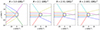 |
Fig. 1. Null geodesics in the equatorial plane of static spherical reflecting surfaces of different radii R. The impact parameter b ranges from −5 to 5 GM/c2. The solid grey line indicates the surface and the dashed grey line the location where the event horizon would have been. |
The first thing to notice, is that there is symmetry in the x-axis. This is because of the absence of the frame-dragging effect and is a logical result of the spherical symmetry. Geodesics with impact parameters ±b will therefore describe the same behavior.
On the left plot, geodesics are shown around a surface of radius R = 3.0 GM/c2, which corresponds to the photon sphere. This means that geodesics with impact parameters smaller than the photon capture radius  reach the surface and are reflected. Geodesics with impact parameter larger than the photon capture radius do not reach the surface nor the photon sphere and are thus the same as geodesics with the same impact parameter around a static black hole. This behavior is true for all surface radii smaller than the radius of the photon sphere.
The geodesics for b = ±1 on the left plot look like the reflection off a reflecting ball in flat spacetime; straight lines in and out. This is expected for geodesics with small impact parameters b reflecting of surfaces with large radii R, since in these cases the geodesics move mostly radially and do not or only briefly go through a region of strong gravity. Indeed, for larger impact parameters b = ±3 and b = ±5, the geodesics are increasingly more curved. This results for b = ±3 in a smaller and for b = ±5 in a larger deflection angle than that of a ball in flat spacetime. Increasing the impact parameter further would result in increasingly larger deflection angles, where the geodesic will orbit the surface many times. The deflection angle will diverge when going to the photon capture radius  , which corresponds to a geodesic that asymptotically converges to a circular photon orbit.
For smaller radii, the deflection angles increasingly become larger as can be seen in the other plots in Fig. 1. This is a result of the fact that the geodesics have to travel farther to reach the surface. It can be seen that even the geodesic with b = ±1 deflects a bit now as expected.
The deflection angle seems to converge when decreasing the radius, with smaller impact parameters nearing their final deflection angle faster than higher impact parameters. The convergence of the deflection angle is expected, since there is an upper limit on the deflection angle set by two times the angular distance to reach the event horizon radius 2GM/c2. The lower impact parameters converge faster because their corresponding geodesics have to travel a smaller angular distance.
3.3. Rotating surfaces
Null geodesics around a rotating reflecting surface are shown in Fig. 2. They are directed towards a far-away observer with inclination i = 60°. The frame-dragging effect causes the geodesics to get dragged along the spin axis resulting in spiraling behavior. Unlike the static case, the geodesics generally do not stay in an orbital plane. The exception are geodesics in the equatorial plane. To get a better understanding of the behavior of the geodesics, we take a look at these. Geodesics in the equatorial plane around a reflecting surface with different radii R are shown in Fig. 3 and with different spin a in Fig. 4.
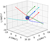 |
Fig. 2. Null geodesics around a rotating reflecting surface with spin a = 0.94 and surface radius R = 1.01 r+, where r+ is the radius an event horizon with the corresponding spin would have had. The geodesics are directed towards a far-away observer in the negative x-direction having an inclination i = 60°. The image plane parameters (α, β) are (2, 2), (2, −2), ( − 2, 2) and ( − 2, −2) GM/c2. |
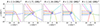 |
Fig. 3. Null geodesics in the equatorial plane of rotating reflecting surfaces of different radii R and with spin a = 0.99. The radii correspond from left to right to 2.0, 1.5, 1.1, 1.01 and 1.001 times the radius r+ an event horizon would have had. The impact parameter b ranges from −5 to 5 GM/c2. The solid grey line indicates the surface and the dashed grey line the location where the event horizon would have been. |
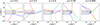 |
Fig. 4. Null geodesics in the equatorial plane of rotating reflecting surfaces of different spin a and with surface radius R = 1.01 r+, where r+ is the radius an event horizon with the corresponding spin would have had. The impact parameter b ranges from −5 to 5 GM/c2. The solid grey line indicates the surface and effectively coincides with the location where the event horizon would have been because of the high spin. |
First of all, it can directly be seen that in the rotating case, there is no symmetry in the x-axis anymore. This is because moving clockwise and anticlockwise is different due to the frame-dragging effect. Geodesics with impact parameters ±b will therefore not describe the same behavior anymore.
In the second plot in Fig. 3, one can see that the line with impact parameter b = −5 has some interesting behavior: it makes a loop. It starts on the right moving anti-clockwise, then switches direction to moving clockwise, reflects and finally switches direction again to finally move anti-clockwise again. At first sight, this seems like strange behavior, since it changes to the anti-clockwise direction after being reflected in the clockwise direction. However, this is a misconception caused by the coordinates. In the ZAMO frame of the reflection point, the reflection happens in the anti-clockwise direction. In the coordinate system of the static observer, it only looks like the reflection is in the other direction, but one has to take the frame-dragging into account to fully appreciate what happens. When the geodesic moves inward, it is dragged along with the spacetime more and more. At a certain moment, it is dragged along more in the anti-clockwise direction than it can move clockwise, which results in a total anti-clockwise motion in the coordinate frame. This is also the case directly after the reflection. Then when it moves further away from the surface, the frame-dragging effect decreases again until the geodesics move clockwise in the coordinate frame again.
The photon orbit changes with spin. In the rotating case, there are two, one prograde (+) and one retrograde (−). Their radius  is given by Bardeen et al. (1972):
![Mathematical equation: $$ \begin{aligned} r_{\rm ph}^{\pm } = 2 \frac{GM}{c^2} \left[1 + \cos \left(\frac{2}{3} \arccos ({\mp }|a|)\right)\right]. \end{aligned} $$](/articles/aa/full_html/2024/09/aa48489-23/aa48489-23-eq38.gif) (18)
(18)
The corresponding shadow radii in the equatorial plane are a bit larger and will for the following discussion be denoted by b±. For  , the geodesics corresponding to impact parameters b ∈ (−b−,b+) will reach the surface and be reflected. Geodesics corresponding to impact parameters b outside [ − b−, b+] do not reach the surface nor the photon orbit and are thus the same as geodesics with the same parameter around a rotating black hole with spin a.
For  , the surface extends for prograde orbits above the photon radius. This means that prograde orbits are different from those around a black hole and that geodesics corresponding to impact parameters
  reach the surface, where
  is the new boundary impact parameter. The transition between these two cases can be seen in Fig. 3 for impact parameter b = 3. In the first plot, it reflects from the surface, but in the later plots, it does not.
For differing spin, it is important to note that the radius of the horizon r+ and therefore of the surface radius R = 1.01 r+ as well decrease with spin. The photon radius for prograde orbits  will also decrease, which can be seen for impact parameters b = 5 and b = 3. In the first plot, they reflect from the surface, but in the later plots, they do not. For retrograde orbits, the photon radius increases, resulting in a larger range of impact parameters falling to the surface. Finally, when increasing the spin to 1 both the radius of the event horizon r+ and the radius of the prograde photon orbit
  will converge to the same value. This means that for spins very close to 1, the radius of the surface R will become higher than the prograde photon orbit
  (
( , giving
  ). So for these spin values there will be prograde geodesics, that are reflected outside the photon sphere.
Just as in the static case, one would expect the deflection angles to converge when decreasing the radius. This only seems to happen for the geodesics with impact parameters b = 5 and b = 3 because these do not reach the surface for smaller radii. It is expected that it takes very small radii to converge, because the frame-dragging causes the geodesics to travel long angular distances as can be seen in the plots. There should, however, be geodesics with small deflection angles that consequently should converge already at relatively large radii. Since the angular deflection continuously goes from −∞ for b− towards +∞ for b+, there should be a b ∈ (b−, b+) such that the deflection angle is 0.
For the spin, in Fig. 4, there is no clear convergent behavior with increasing spin visible. Just like in the case with decreasing radius, one would expect convergence of the geodesics when increasing the spin to a = 1, since it changes continuously to 1 and there is a specific solution for a = 1. Again, the convergence will be faster for impact parameters with small deflection angles.
Coming back to the general case for orbits outside the equatorial plane, similar behaviour is expected, but now with orbital motion in the θ-direction as well. Just as before, geodesics will fall to the surface when going below the photon orbit and be reflected. For large surface radii, the surface can (partly) stick above the photon orbits, resulting in reflected geodesics there as well. We also expect similar converging behaviour for surface radius R to event horizon radius r+ and spin a going to 1.
4. Synthetic images
4.1. Method
To make synthetic images, we use a modified version of the general radiative transfer code RAPTOR (Bronzwaer et al. 2018). It calculates null geodesics and integrates the relativistic radiative transfer equation along them. To use it for synthetic images of reflecting surfaces, we modified the calculation of the geodesics in the same way as discussed in Sect. 3.1. The radiative transfer is subsequently integrated along the reflected geodesic.
The only difference in the calculation of the geodesics compared to Sect. 3.1, is that we use modified Kerr-Schild coordinates as defined for the GRMHD code BHAC (Porth et al. 2017) instead of Boyer-Lindquist coordinates. This means that the reflection law generally does not work anymore, since Eq. (17) is in Boyer-Lindquist coordinates. To solve this, when calculating the reflection, the wave vector is transformed to Boyer-Lindquist coordinates, reflected using Eq. (17) and then transformed back.
The synthetic images have a field of view of 30 × 30 GM/c2 with resolution of 1000 × 1000 pixels for the analytic Keplerian torus model and 256 × 256 pixels for the GRMHD models. An observing frequency of 230 GHz is used, at which the gas is optically thin.
4.2. Analytic keplerian torus model
To build insight into the structure of synthetic images with a rotating reflecting surface, we first look at an analytic model of a Keplerian torus. The model is described in Appendix A of Davelaar et al. (2019). We use a single torus in the equatorial plane with radius rring = 5 GM/c2 and cross-sectional thickness of 1 GM/c2. The model is perfectly optically thin (so absorption is not taken into account) and we use as emissivity profile a step-function that is 1 inside the torus and 0 outside it. Additionally, a Keplerian velocity vector is given to the material, to take the relativistic boosting effect into account. Synthetic images for different surface radii R are shown in Fig. 5 and for different spins a in Fig. 6. In Fig. 7, synthetic images with several spins a and i are shown, which will be used in the GRMHD models as well.
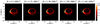 |
Fig. 5. Synthetic images of rotating reflecting surfaces with different radii R, with spin a = 0.99, inclination i = 60° and surrounded by an analytic Keplerian torus. The radii correspond from left to right to 2.0, 1.5, 1.1, 1.01 and 1.001 times the radius r+ an event horizon would have had. |
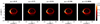 |
Fig. 6. Synthetic images of rotating reflecting surfaces with different spin a, inclination i = 60° and surrounded by an analytic Keplerian torus. The surface radius is R = 1.01 r+, where r+ is the radius an event horizon with the corresponding spin would have had. |
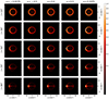 |
Fig. 7. Synthetic images of rotating reflecting surfaces with different spin a and inclination i, surrounded by an analytic Keplerian torus. The surface radius is R = 1.01 r+, where r+ is the radius an event horizon with the corresponding spin would have had. |
First of all, one can see the lensed image of the torus and subsequent higher order lensed images interior to that converging to the photon sphere. The latter corresponds to geodesics orbiting the surface increasingly many times.
Then we immediately see, that in all images, a ring in the center and several (partial) rings subsequently exterior to that can be seen. These are reflected images of the emitting torus in the rotating reflecting surface. The central ring corresponds to the direct reflection, with which we mean that the geodesic has a deflection angle in the θ-direction around 0. The subsequent rings outside that, correspond to geodesics with deflection angles in the θ-direction of half-integer multiples of an orbit larger. This is expected from the results of Sect. 3. Around the middle, there should be a geodesic with deflection angle 0 and when going outwards toward the photon ring, the deflection angle will increase or decrease depending on the side.
The number of rings depends on the surface radius R and spin a, since those decide whether or not the surface radius R lies (partially) outside the photon sphere or not. In Fig. 5, one can see in the first two plots, that not all rings are full. In the first plot, all rings except the central one are open in the top-left. In the second plot, the first ring exterior to the central ring has become full, but the next rings are open in the top-right. This is because the surface lies outside the photon sphere there and limits the possible angular distance geodesics can travel, thereby blocking higher-order rings. In the later plots, the surfaces sink below the photon sphere and an infinite amount of rings are created converging to the photon sphere. Similar behavior is possible by increasing the spin, where part of the surface can start lying above the photon sphere from a certain spin and higher.
In Fig. 5, we see that the size of the rings decreases when the radius decreases. The rings seem to converge in the later plots. This is expected, since geodesics with low deflection angles converge fast with decreasing radius.
In Fig. 6, we see that the sizes of the rings decrease and that their shape change. The first is caused by the fact that the radius decreases with higher spin. The second is because of the frame-dragging. On the left, the rings are close to the center, caused by geodesics moving along with the rotation. On the right, the rings are farther from the center, caused by geodesics moving against the rotation. The rings seem to converge in the later plots. This is expected again, since geodesics with low deflection angles converge fast with increasing spin.
In Fig. 7, images are shown with a negative spin, meaning that the rotation of the surface is the opposite of that of the torus. Here, the structure of the rings is mirrored from that of positive spins.
Also, different inclinations are shown. It can be seen that for low inclinations, the rings are almost concentric circles, which is expected from the symmetry in the spin axis.
4.3. General relativistic magnetohydrodynamical model
Now that we understand the structure of synthetic images of rotating reflecting surfaces, we move on to a more realistic model: a GRMHD simulation. For this, SANE 3D-GRMHD simulations by the GRMHD code BHAC (Porth et al. 2017; Olivares et al. 2019) were used that were made for the EHT GRMHD simulation library (Event Horizon Telescope Collaboration 2019a). The simulations have spins a ∈ {0, ± 0.5, ± 0.9375}. As initial condition a Fishbone-Moncrief torus Fishbone & Moncrief (1976) is used of which the rotation axis is aligned with the spin axis of the black hole. A numerical grid with three spatial coordinates r, θ and ϕ is used in spherical modified Kerr-Schild coordinates. The simulation domain ranges from the horizon to a radius of 3333 GM/c2. The spatial resolution of the grid is Nr × Nθ × Nϕ = 512 × 192 × 192.
It is important to emphasize that these are simulations of black holes, not surfaces. As described earlier, the surface is ‘added’ in the radiative transfer code. Since the calculated geodesics are not allowed inside of the surface, the region inside the surface radius R is essentially cut out. Because the GRMHD simulations do not contain a surface, the effects of deceleration of material falling onto the surface are not taken into account. Emission related to heating of the surface due to the release of kinetic energy by the infalling matter has also been neglected, in line with a scenario of a surface with a very large heat capacity as it is assumed for certain black hole mimickers (Mazur & Mottola 2004).
The emission model that is used here is that of synchrotron emission and self-absorption based on the properties of the plasma as calculated in the GRMHD simulation. The images are integrated over a simulation time from t = 9500 − 10 000 M by taking the average over 51 snapshots separated 10 M in time each. The electron temperature description from Mościbrodzka et al. (2016) is used with Rhigh = 3. This is chosen to reflect the analytic Keplerian torus model and to guarantee good sight at the shadow region. Reflecting features are expected for large values of Rhigh as well, so when the emission is jet-dominated, but may be more obscured by the jet. We use the mass and distance to Sgr A* and fit the accretion rate by demanding an integrated flux of 2.4 Jy at 230 GHz. In Fig. 8, synthetic images are shown for different surface radii R. In Fig. 9, synthetic images with several spins a and i are shown. Fig. 8 can be compared to Figs. 5 and 7 with Fig. 9.
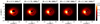 |
Fig. 8. Synthetic images of rotating reflecting surfaces with different radii R, with spin a = 0.99, inclination i = 60° and using a SANE GRMHD model. The radii correspond from left to right to 2.0, 1.5, 1.1, 1.01 and 1.001 times the radius r+ an event horizon would have had. |
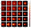 |
Fig. 9. Synthetic images of rotating reflecting surfaces with different spin a and inclination i, using a SANE GRMHD model. The surface radius is R = 1.01 r+, where r+ is the radius an event horizon with the corresponding spin would have had. |
Again, we clearly see the accretion disk, a central ring and several rings exterior to that. The sizes, shapes and positions are mostly the same as those for the analytic Keplerian torus model. The central ring in the images of the GRMHD model seems to be a bit thicker. This is caused by the geometrically thicker accretion disk.
New in the images from the GRMHD model is the clear flux distribution. Surprisingly, the central ring is now the brightest object in the image. This is caused by Doppler-boosting of the gas rushing in radially towards the surface. Normally, this high intensity light is not seen because it ends up falling in the horizon. In this case, however, the light is reflected and able to escape. This radial boosting effect can be shown to be the explanation in three ways. Firstly, the brightening of the ring cannot be seen in the analytic torus model, which has as main difference with the GRMHD model that the gas has no radial velocity. Secondly, from Narayan et al. (2019) it is known that inward radial velocity enhances the depth of the shadow of a black hole. When you include a reflecting surface, the post-reflecting segment of the geodesic (when tracing backwards in time) sees radiating gas moving rapidly “towards” the observer, so we expect a huge boost. Thirdly, when separating the contributions to the intensity from the pre- and post-reflection parts of the geodesic, you clearly see the intensity is dominated by the post-reflection intensity.
In most images, the central ring is brighter on the left side. This is caused by Doppler boosting just as in the accretion disk. The exception to this behavior are the images with spin a = −0.9375. Here the ring is the brightest on the bottom. We speculate that this behaviour is caused by the retrograde motion of the accretion disk canceling the boosting effect of spacetime to a large degree.
In addition to the central ring, again higher order rings exterior to the central one can be distinguished.
All these images were averaged to clearly show the reflecting features. However, accretion near supermassive black holes is highly variable. It is therefore interesting to look at an image using only a single snapshot as well. This is shown in Fig. 10 for a snapshot at time 10 000 M and with a resolution of 1000 × 1000 pixels. To study the influence of frequency and optical depth, the image is shown for frequencies of respectively 230 GHz and 2.3 THz and with respectively the absorption on and off. For completeness, to compare the images to those of a black hole, also images with absorption off and without a surface are shown.
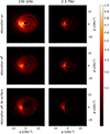 |
Fig. 10. Synthetic images using one snapshot of a SANE GRMHD model of a rotating reflecting surface with the absorption on and off and a black hole with the absorption off for two frequencies. The spin is a = 0.9375. The radius of the surface is R = 1.01 r+, where r+ is the radius an event horizon with the corresponding spin would have had. The inclination is i = 60°. |
Firstly, the images are less smooth than averaged images and show a lot more structure in the accretion disk and its reflections. Despite this, the central ring and some higher-order rings are clearly visible. To some extent, it is even possible to couple structures in the accretion disk with their reflected version. This would lead to interesting light echoes. For surface locations close enough to r+, the travel time of photons will be larger than any variability timescale. However, in the case of a (close to) optically thin source, this does not affect the locations of the rings, because these are only set by the geometry of spacetime.
To study the optical depth, one can compare the images of the reflecting surfaces with the absorption on and off. At 230 GHz, one sees that the image is (somewhat) optically thick in some regions. However, it is expected that these regions will become optically thin when increasing the frequency. This is exactly what can be seen in the images at 2.3 THz where there is almost no difference anymore between having the absorption on and off.
Finally, when comparing the two frequencies, one can see that at a higher frequency the reflection becomes the dominate feature in the image. This trend continues for higher frequencies. This means that for a reflecting surface and black hole with the same intensity at 230 GHz, the intensity at higher frequencies will be higher for reflecting surfaces. So reflecting surface models are a way to increase the spectrum of black hole candidates at higher frequencies.
5. Discussion
5.1. Static spherical surfaces
We can compare our results on static spherical reflecting surfaces with those in Event Horizon Telescope Collaboration (2022c) and Carballo-Rubio et al. (2022). In Event Horizon Telescope Collaboration (2022c), the reflection law given in Eq. (1) was used. This is the exact same reflection law that we used, namely Eq. (11). The latter was derived from a general description for reflecting surfaces in arbitrary spacetimes. This strengthens our confidence in the correctness of the model and gives context and insight into its origin and validity.
For the synthetic images, Event Horizon Telescope Collaboration (2022c) used a long-duration simulation of a hot accretion flow in the MAD state around a black hole with spin a = 0 (Narayan et al. 2022) averaged over a long timescale. For the electron temperature the same prescription as here was used with parameter values Rhigh = 20 and Rlow = 1. Likewise, the accreting gas density was scaled such that the observed flux density at 230 GHz is equal to 2.4 Jy. Finally, an inclination of i = 60° and a reflecting surface radius of R = 2.5 GM/c2 were used. An image with albedo A = 1 can be seen on the left in the second row of Fig. 15 in Event Horizon Telescope Collaboration (2022c).
Carballo-Rubio et al. (2022) used a semi-analytic geometrically thin, optically thick equatorial Keplerian disk. Images of a reflecting surface with different radii and inclinations of respectively i = 0° and i = 60° can be seen in Figs. 1 and 2 in Carballo-Rubio et al. (2022).
We can compare these images to the first image in Fig. 6 and the images in the central column of Figs. 7 and 9. Apart from the surrounding accreting material, the images look very similar. In both images, a bright central ring and a second ring exterior to that are clearly visible. The position, shape, size and flux distribution along the rings are the same. This is all despite the use of different accretion and emission models. This gives confidence in the validity and generality of both results.
5.2. Comparison static and rotating surfaces
We developed a model for rotating reflecting surfaces with the corresponding reflection law given in Eq. (17). Surprisingly enough, this is the same as that for static surfaces: Eq. (11). This result depends of course on the coordinates used; the Boyer-Lindquist coordinates are coordinates that nicely extend the reflection law from the static to the rotating case. Here one has to remind oneself that the model for the rotating surface is an approximation and the reflection law may be different for a metric and surface of a specific mass distribution.
The synthetic images showed that in the rotating case, we see again ring-like features inside the photon ring. The location, shape, size and flux distribution along the ring depend on the radius of the surface R, spin a and inclination i. However, in all cases, there is a bright ring in the middle of the ‘shadow region’ and one or more clearly visible rings exterior to that as well.
The ring features are the result of specular reflection. In the case of diffuse reflection, we could imagine the images to be totally different. At first sight, we would expect the surface to radiate in all directions, resulting in the illumination of the whole shadow region. There might be some substructure there caused by the accretion disk illuminating different parts of the surface more than others, but the ring features found here will probably be gone. If the light is reflected off some sort of atmosphere, we would expect the reflected light to be diffuse as well, but still mainly directed close to the direction of specular reflected light. In that case, we would expect the images to still have the ring features, although the rings will probably become a bit thicker.
5.3. Implications for the event horizon telescope
Since the image features of rotating reflecting surfaces are similar to those of static ones, the argument presented in Event Horizon Telescope Collaboration (2022c) should still hold when allowing rotation. This means that for high albedo, reflecting surfaces and event horizons should be distinguishable, even with a 15 μas blur, and consequently that such reflecting surface models are unlikely given the EHT observations. Given that absorbing surfaces have been mostly excluded as well, this strengthens the conclusion that the shadow indeed indicates the existence of an event horizon.
However, Carballo-Rubio et al. (2022) is more pessimistic about the possibility to exclude models with the current dynamic range. In their synthetic images, the reflected rings are less bright relative to the accretion disk and therefore not distinguishable when introducing a blur. The difference in brightness of the reflected rings can be explained by the fact that they use a semi-analytic Keplerian disk model, in which the accreting material does not have any radial motion, preventing the radial boosting effect. We would argue that taking this effect into account is more realistic. However, it is good to emphasize that the argument given by Event Horizon Telescope Collaboration (2022c) depends on the used accretion model. Increasing the dynamic range would allow us to test the model in Carballo-Rubio et al. (2022) as well.
Of course, it should be mentioned that the model discussed in this paper is still a toy model and still much can be improved to make more realistic models of exotic compact objects with rotating reflecting surfaces. We also note that these kinds of models might be interesting in the context of neutron stars, which are thought to have (highly) reflecting surfaces (Lenzen & Truemper 1978).
6. Conclusion
In this paper, we looked at rotating reflecting surfaces in the context of testing the existence of event horizons using horizon-scale images of black holes. We have developed a general description of reflecting surfaces in arbitrary spacetimes and used this to define specific models for static spherical surfaces and rotating surfaces. The reflecting surfaces create an infinite set of ring-like features in synthetic images inside the photon ring. There is a bright central ring in the middle and higher order rings subsequently lie exterior to each other converging to the photon ring. The shape and size of the ring features change only slightly with the radius of the surface R, spin a and inclination i. In all cases, this results in features inside the middle of the ‘shadow region’. We conclude that rotating reflecting surfaces have clear observable features and that the Event Horizon Telescope might be able to observe the difference between reflecting surfaces and an event horizon. Reflecting surfaces with high reflectivities seem unlikely. Together with the exclusion of absorbing surfaces, this strengthens the case that the shadow indeed indicates the existence of an event horizon.
Acknowledgments
We thank Luciano Rezzolla for insightful comments regarding this research. We also thank Christiaan Brinkerink, Jesse Vos, Jordy Davelaar and Joris Kersten for helpful discussions. Finally, we want to thank the anonymous EHT Collaboration internal reviewer and A&A peer reviewer for helpful comments. This work is supported by the Radboud University and the ERC Synergy Grant ‘Blackholistic’. YM is supported by the National Natural Science Foundation of China (No. 12273022) and the Shanghai target program of basic science research for international scientists (No. 22JC1410600). HO is supported by the Center for Research and Development in Mathematics and Applications (CIDMA) through the Portuguese Foundation for Science and Technology (FCT – Fundação para a Ciência e a Tecnologia), references UIDB/04106/2020, UIDP/04106/2020. HO acknowledges support from the projects PTDC/FIS-AST/3041/2020, CERN/FIS-PAR/0024/2021 and 2022.04560.PTDC. HO has further been supported by the European Union’s Horizon 2020 research and innovation (RISE) programme H2020-MSCA-RISE-2017 Grant No. FunFiCO-777740 and by the European Horizon Europe staff exchange (SE) programme HORIZON-MSCA-2021-SE-01 Grant No. NewFunFiCO-10108625. During part of this project, funding for HO came from Radboud University Nijmegen through a Virtual Institute of Accretion (VIA) postdoctoral fellowship from the Netherlands Research School for Astronomy (NOVA). HO is supported by the Individual CEEC program – 5th edition funded by the Portuguese Foundation for Science and Technology (FCT).
References
- Abbott, B. P., Abbott, R., Abbott, T. D., et al. 2016, Phys. Rev. Lett., 116, 061102 [Google Scholar]
- Abbott, R., Abbott, T. D., Abraham, S., et al. 2021, Phys. Rev. D, 103, 122002 [NASA ADS] [CrossRef] [Google Scholar]
- Andréasson, H. 2008, J. Diff. Eq., 245, 2243 [CrossRef] [Google Scholar]
- Bardeen, J. M., Press, W. H., & Teukolsky, S. A. 1972, ApJ, 178, 347 [Google Scholar]
- Birkhoff, G. 1923, Relativity and Modern Physics (Cambridge: Harvard University Press) [Google Scholar]
- Blandford, R. D., & Znajek, R. L. 1977, MNRAS, 179, 433 [NASA ADS] [CrossRef] [Google Scholar]
- Bolotovskiĭ, B. M., & Stolyarov, S. N. 1989, Sov. Phys. Usp., 32, 813 [CrossRef] [Google Scholar]
- Bolton, C. T. 1972, Nature, 235, 271 [NASA ADS] [CrossRef] [Google Scholar]
- Broderick, A. E., & Narayan, R. 2006, ApJ, 638, L21 [Google Scholar]
- Broderick, A. E., & Narayan, R. 2007, Class. Quant. Grav., 24, 659 [CrossRef] [Google Scholar]
- Broderick, A. E., Loeb, A., & Narayan, R. 2009, ApJ, 701, 1357 [NASA ADS] [CrossRef] [Google Scholar]
- Bronzwaer, T., & Falcke, H. 2021, ApJ, 920, 155 [NASA ADS] [CrossRef] [Google Scholar]
- Bronzwaer, T., Davelaar, J., Younsi, Z., et al. 2018, A&A, 613, A2 [NASA ADS] [CrossRef] [EDP Sciences] [Google Scholar]
- Buchdahl, H. A. 1959, Phys. Rev., 116, 1027 [NASA ADS] [CrossRef] [Google Scholar]
- Carballo-Rubio, R., Cardoso, V., & Younsi, Z. 2022, Phys. Rev. D, 106, 084038 [NASA ADS] [CrossRef] [Google Scholar]
- Cardoso, V., & Pani, P. 2017, ArXiv e-prints [arXiv:1709.01525] [Google Scholar]
- Cardoso, V., & Pani, P. 2019, Liv. Rev. Relat., 22, 4 [NASA ADS] [CrossRef] [Google Scholar]
- Cardoso, V., Franzin, E., & Pani, P. 2016a, Phys. Rev. Lett., 116, 171101 [NASA ADS] [CrossRef] [Google Scholar]
- Cardoso, V., Hopper, S., Macedo, C. F. B., Palenzuela, C., & Pani, P. 2016b, Phys. Rev. D, 94, 084031 [NASA ADS] [CrossRef] [Google Scholar]
- Carter, B. 1968, Phys. Rev., 174, 1559 [Google Scholar]
- Carter, B. 1971, Phys. Rev. Lett., 26, 331 [NASA ADS] [CrossRef] [Google Scholar]
- Cunha, P. V. P., & Herdeiro, C. A. R. 2018, Gen. Relat. Grav., 50, 42 [CrossRef] [Google Scholar]
- Cunningham, C. T., & Bardeen, J. M. 1973, ApJ, 183, 237 [Google Scholar]
- Davelaar, J., Olivares, H., Porth, O., et al. 2019, A&A, 632, A2 [NASA ADS] [CrossRef] [EDP Sciences] [Google Scholar]
- Do, T., Hees, A., Ghez, A., et al. 2019, Science, 365, 664 [Google Scholar]
- Einstein, A. 1905, Ann. Phys., 322, 891 [NASA ADS] [CrossRef] [Google Scholar]
- Einstein, A. 1915, Sitzungsberichte der Königlich Preußischen Akademie der Wissenschaften (Berlin), 844 [Google Scholar]
- Event Horizon Telescope Collaboration (Akiyama, K., et al.) 2019a, ApJ, 875, L1 [Google Scholar]
- Event Horizon Telescope Collaboration (Akiyama, K., et al.) 2019b, ApJ, 875, L5 [Google Scholar]
- Event Horizon Telescope Collaboration (Akiyama, K., et al.) 2019c, ApJ, 875, L6 [Google Scholar]
- Event Horizon Telescope Collaboration (Akiyama, K., et al.) 2022a, ApJ, 930, L12 [NASA ADS] [CrossRef] [Google Scholar]
- Event Horizon Telescope Collaboration (Akiyama, K., et al.) 2022b, ApJ, 930, L16 [NASA ADS] [CrossRef] [Google Scholar]
- Event Horizon Telescope Collaboration (Akiyama, K., et al.) 2022c, ApJ, 930, L17 [NASA ADS] [CrossRef] [Google Scholar]
- Fabian, A. C. 2012, ARA&A, 50, 455 [Google Scholar]
- Falcke, H., & Biermann, P. L. 1999, A&A, 342, 49 [NASA ADS] [Google Scholar]
- Falcke, H., Melia, F., & Agol, E. 2000, ApJ, 528, L13 [Google Scholar]
- Fishbone, L. G., & Moncrief, V. 1976, ApJ, 207, 962 [NASA ADS] [CrossRef] [Google Scholar]
- Frolov, A. V., & Frolov, V. P. 2014, Phys. Rev. D, 90, 124010 [NASA ADS] [CrossRef] [Google Scholar]
- Galli, J. R., & Amiri, F. 2012, Am. J. Phys., 80, 680 [Google Scholar]
- Gjurchinovski, A. 2004, Am. J. Phys., 72, 1316 [Google Scholar]
- Goddi, C., Falcke, H., Kramer, M., et al. 2017, Int. J. Mod. Phys. D, 26, 1730001 [Google Scholar]
- GRAVITY Collaboration (Abuter, R., et al.) 2018, A&A, 615, L15 [NASA ADS] [CrossRef] [EDP Sciences] [Google Scholar]
- GRAVITY Collaboration (Abuter, R., et al.) 2020, A&A, 636, L5 [NASA ADS] [CrossRef] [EDP Sciences] [Google Scholar]
- Harlow, D. 2016, Rev. Mod. Phys., 88, 015002 [NASA ADS] [CrossRef] [Google Scholar]
- Hawking, S. W. 1972, Commun. Math. Phys., 25, 152 [Google Scholar]
- Hawking, S. W. 1975, Commun. Math. Phys., 43, 199 [CrossRef] [Google Scholar]
- Israel, W. 1967, Phys. Rev., 164, 1776 [Google Scholar]
- Israel, W. 1968, Commun. Math. Phys., 8, 245 [CrossRef] [Google Scholar]
- Jackson, J. D. 1999, Classical Electrodynamics, 3rd edn. (New York: Wiley) [Google Scholar]
- Jaroszynski, M., & Kurpiewski, A. 1997, A&A, 326, 419 [Google Scholar]
- Johannsen, T., & Psaltis, D. 2010, ApJ, 718, 446 [NASA ADS] [CrossRef] [Google Scholar]
- Kerr, R. P. 1963, Phys. Rev. Lett., 11, 237 [Google Scholar]
- Kocherlakota, P., & Rezzolla, L. 2022, MNRAS, 513, 1229 [NASA ADS] [CrossRef] [Google Scholar]
- Kormendy, J., & Ho, L. C. 2013, ARA&A, 51, 511 [Google Scholar]
- Lenzen, R., & Truemper, J. 1978, Nature, 271, 216 [NASA ADS] [CrossRef] [Google Scholar]
- Luminet, J. P. 1979, A&A, 75, 228 [Google Scholar]
- Lynden-Bell, D. 1969, Nature, 223, 690 [NASA ADS] [CrossRef] [Google Scholar]
- Magorrian, J., Tremaine, S., Richstone, D., et al. 1998, AJ, 115, 2285 [Google Scholar]
- Mazur, P. O., & Mottola, E. 2004, Proc. Natl. Acad. Sci. USA, 101, 9545 [CrossRef] [PubMed] [Google Scholar]
- McClintock, J. E., & Remillard, R. A. 1986, ApJ, 308, 110 [Google Scholar]
- Mościbrodzka, M., Falcke, H., & Shiokawa, H. 2016, A&A, 586, A38 [Google Scholar]
- Nagar, N. M., Wilson, A. S., & Falcke, H. 2001, ApJ, 559, L87 [NASA ADS] [CrossRef] [Google Scholar]
- Narayan, R. 2002, in Lighthouses of the Universe: The Most Luminous Celestial Objects and Their Use for Cosmology, eds. M. Gilfanov, R. Sunyeav, & E. Churazov, 405 [CrossRef] [Google Scholar]
- Narayan, R., & McClintock, J. E. 2008, New Astron Rev., 51, 733 [NASA ADS] [CrossRef] [Google Scholar]
- Narayan, R., Mahadevan, R., & Quataert, E. 1998a, in Theory of Black Hole Accretion Disks, eds. M. A. Abramowicz, G. Björnsson, & J. E. Pringle, 148 [Google Scholar]
- Narayan, R., Mahadevan, R., Grindlay, J. E., Popham, R. G., & Gammie, C. 1998b, ApJ, 492, 554 [Google Scholar]
- Narayan, R., Johnson, M. D., & Gammie, C. F. 2019, ApJ, 885, L33 [Google Scholar]
- Narayan, R., Chael, A., Chatterjee, K., Ricarte, A., & Curd, B. 2022, MNRAS, 511, 3795 [NASA ADS] [CrossRef] [Google Scholar]
- Olivares, H., Porth, O., Davelaar, J., et al. 2019, A&A, 629, A61 [NASA ADS] [CrossRef] [EDP Sciences] [Google Scholar]
- Olivares, H., Younsi, Z., Fromm, C. M., et al. 2020, MNRAS, 497, 521 [Google Scholar]
- Oppenheimer, J. R., & Snyder, H. 1939, Phys. Rev., 56, 455 [Google Scholar]
- Ozel, F., Psaltis, D., & Younsi, Z. 2021, ArXiv e-prints [arXiv:2111.01123] [Google Scholar]
- Penrose, R. 1965, Phys. Rev. Lett., 14, 57 [NASA ADS] [CrossRef] [Google Scholar]
- Penrose, R. 1969, Nuovo Cimento Rivista Serie, 1, 252 [NASA ADS] [Google Scholar]
- Penrose, R., & Floyd, R. M. 1971, Nat. Phys. Sci., 229, 177 [NASA ADS] [CrossRef] [Google Scholar]
- Porth, O., Olivares, H., Mizuno, Y., et al. 2017, Comput. Astrophys. Cosmol., 4, 1 [Google Scholar]
- Price, R. H. 1972a, Phys. Rev. D, 5, 2419 [NASA ADS] [CrossRef] [Google Scholar]
- Price, R. H. 1972b, Phys. Rev. D, 5, 2439 [CrossRef] [Google Scholar]
- Psaltis, D. 2019, Gen. Relat. Grav., 51, 137 [CrossRef] [Google Scholar]
- Psaltis, D., & Johannsen, T. 2011, J. Phys. Conf. Ser., 283, 012030 [NASA ADS] [CrossRef] [Google Scholar]
- Psaltis, D., Wex, N., & Kramer, M. 2016, ApJ, 818, 121 [Google Scholar]
- Richstone, D., Ajhar, E. A., Bender, R., et al. 1998, Nature, 385, A14 [Google Scholar]
- Robinson, D. C. 1975, Phys. Rev. Lett., 34, 905 [CrossRef] [Google Scholar]
- Schmidt, M. 1963, Nature, 197, 1040 [Google Scholar]
- Schwarzschild, K. 1916, Abh. Konigl. Preuss. Akad. Wissenschaften Jahre, 1916, 189 [Google Scholar]
- van der Gucht, J., Davelaar, J., Hendriks, L., et al. 2020, A&A, 636, A94 [EDP Sciences] [Google Scholar]
- Vincent, F. H., Wielgus, M., Abramowicz, M. A., et al. 2021, A&A, 646, A37 [NASA ADS] [CrossRef] [EDP Sciences] [Google Scholar]
- Webster, B. L., & Murdin, P. 1972, Nature, 235, 37 [Google Scholar]
- Younsi, Z., Zhidenko, A., Rezzolla, L., Konoplya, R., & Mizuno, Y. 2016, Phys. Rev. D, 94, 084025 [Google Scholar]
All Figures
|
Fig. 1. Null geodesics in the equatorial plane of static spherical reflecting surfaces of different radii R. The impact parameter b ranges from −5 to 5 GM/c2. The solid grey line indicates the surface and the dashed grey line the location where the event horizon would have been. |
| In the text | |
|
Fig. 2. Null geodesics around a rotating reflecting surface with spin a = 0.94 and surface radius R = 1.01 r+, where r+ is the radius an event horizon with the corresponding spin would have had. The geodesics are directed towards a far-away observer in the negative x-direction having an inclination i = 60°. The image plane parameters (α, β) are (2, 2), (2, −2), ( − 2, 2) and ( − 2, −2) GM/c2. |
| In the text | |
|
Fig. 3. Null geodesics in the equatorial plane of rotating reflecting surfaces of different radii R and with spin a = 0.99. The radii correspond from left to right to 2.0, 1.5, 1.1, 1.01 and 1.001 times the radius r+ an event horizon would have had. The impact parameter b ranges from −5 to 5 GM/c2. The solid grey line indicates the surface and the dashed grey line the location where the event horizon would have been. |
| In the text | |
|
Fig. 4. Null geodesics in the equatorial plane of rotating reflecting surfaces of different spin a and with surface radius R = 1.01 r+, where r+ is the radius an event horizon with the corresponding spin would have had. The impact parameter b ranges from −5 to 5 GM/c2. The solid grey line indicates the surface and effectively coincides with the location where the event horizon would have been because of the high spin. |
| In the text | |
|
Fig. 5. Synthetic images of rotating reflecting surfaces with different radii R, with spin a = 0.99, inclination i = 60° and surrounded by an analytic Keplerian torus. The radii correspond from left to right to 2.0, 1.5, 1.1, 1.01 and 1.001 times the radius r+ an event horizon would have had. |
| In the text | |
|
Fig. 6. Synthetic images of rotating reflecting surfaces with different spin a, inclination i = 60° and surrounded by an analytic Keplerian torus. The surface radius is R = 1.01 r+, where r+ is the radius an event horizon with the corresponding spin would have had. |
| In the text | |
|
Fig. 7. Synthetic images of rotating reflecting surfaces with different spin a and inclination i, surrounded by an analytic Keplerian torus. The surface radius is R = 1.01 r+, where r+ is the radius an event horizon with the corresponding spin would have had. |
| In the text | |
|
Fig. 8. Synthetic images of rotating reflecting surfaces with different radii R, with spin a = 0.99, inclination i = 60° and using a SANE GRMHD model. The radii correspond from left to right to 2.0, 1.5, 1.1, 1.01 and 1.001 times the radius r+ an event horizon would have had. |
| In the text | |
|
Fig. 9. Synthetic images of rotating reflecting surfaces with different spin a and inclination i, using a SANE GRMHD model. The surface radius is R = 1.01 r+, where r+ is the radius an event horizon with the corresponding spin would have had. |
| In the text | |
|
Fig. 10. Synthetic images using one snapshot of a SANE GRMHD model of a rotating reflecting surface with the absorption on and off and a black hole with the absorption off for two frequencies. The spin is a = 0.9375. The radius of the surface is R = 1.01 r+, where r+ is the radius an event horizon with the corresponding spin would have had. The inclination is i = 60°. |
| In the text | |
Current usage metrics show cumulative count of Article Views (full-text article views including HTML views, PDF and ePub downloads, according to the available data) and Abstracts Views on Vision4Press platform.
Data correspond to usage on the plateform after 2015. The current usage metrics is available 48-96 hours after online publication and is updated daily on week days.
Initial download of the metrics may take a while.