| Issue |
A&A
Volume 612, April 2018
|
|
|---|---|---|
| Article Number | A115 | |
| Number of page(s) | 14 | |
| Section | Galactic structure, stellar clusters and populations | |
| DOI | https://doi.org/10.1051/0004-6361/201732144 | |
| Published online | 08 May 2018 | |
The VMC survey
XXVIII. Improved measurements of the proper motion of the Galactic globular cluster 47 Tucanae★
1
Leibniz-Institut für Astrophysik Potsdam,
An der Sternwarte 16,
14482 Potsdam,
Germany
e-mail: fniederhofer@aip.de
2
University of Hertfordshire, Physics Astronomy and Mathematics,
College Lane, Hatfield AL10 9AB,
UK
3
Osservatorio Astronomico di Padova − INAF,
Vicolo dell’Osservatorio 5,
35122 Padova,
Italy
4
Dipartimento di Fisica e Astronomia,
Universita di Padova,
Vicolo dell’Osservatorio 2,
35122 Padova, Italy
5
ICRAR, M468, University of Western Australia,
35 Stirling Hwy,
6009 Crawley, Western Australia,
Australia
6
Kavli Institute for Astronomy & Astrophysics and Department of Astronomy, Peking University,
Yi He Yuan Lu 5,
Hai Dian District,
Beijing 100871, PR China
7
International Space Science Institute–Beijing,
1 Nanertiao,
Zhongguancun,
Hai Dian District,
Beijing 100190, PR China
8
Astronomy Unit, School of Physics and Astronomy, Queen Mary University of London,
Mile End Road,
London E1 4NS, UK
9
European Southern Observatory,
Ave. Alonso de Córdova 3107,
Vitacura, Santiago, Chile
10
European Southern Observatory,
Karl-Schwarzschild-Str. 2,
85748 Garching bei München,
Germany
11
Lennard-Jones Laboratories, Keele University,
ST5 5BG, UK
12
INAF-Osservatorio Astronomico di Capodimonte,
via Moiariello 16,
80131,
Napoli,
Italy
Received:
20
October
2017
Accepted:
23
January
2018
We use deep multi-epoch point-spread function (PSF) photometry taken with the Visible and Infrared Survey Telescope for Astronomy (VISTA) to measure and analyze the proper motions of stars within the Galactic globular cluster 47 Tucanae (47 Tuc, NGC 104). The observations are part of the ongoing near-infrared VISTA survey of the Magellanic Cloud system (VMC). The data analyzed in this study correspond to one VMC tile, which covers a total sky area of 1.77 deg2. Absolute proper motions with respect to ~9070 background galaxies are calculated from a linear regression model applied to the positions of stars in 11 epochs in the Ks filter. The data extend over a total time baseline of about 17 months. We found an overall median proper motion of the stars within 47 Tuc of (μαcos(δ), μδ) = (+5.89 ± 0.02 (statistical) ± 0.13 (systematic), −2.14 ± 0.02 (statistical) ± 0.08 (systematic)) mas yr−1, based on the measurements of ~35 000 individual sources between 5′ and 42′ from the cluster center. We compared our result to the proper motions from the newest US Naval Observatory CCD Astrograph Catalog (UCAC5), which includes data from the Gaia data release 1. Selecting cluster members ( ~2700 stars), we found a median proper motion of (μαcos(δ), μδ) = (+5.30 ± 0.03 (statistical) ± 0.70 (systematic), −2.70 ± 0.03 (statistical) ± 0.70 (systematic)) mas yr−1. Comparing the results with measurements in the literature, we found that the values derived from the VMC data are consistent with the UCAC5 result, and are close to measurements obtained using the Hubble Space Telescope. We combined our proper motion results with radial velocity measurements from the literature and reconstructed the orbit of 47 Tuc, finding that the cluster is on an orbit with a low ellipticity and is confined within the inner ~7.5 kpc of the Galaxy. We show that the use of an increased time baseline in combination with PSF-determined stellar centroids in crowded regions significantly improves the accuracy of the method. In future works, we will apply the methods described here to more VMC tiles to study in detail the kinematics of the Magellanic Clouds.
Key words: proper motions / surveys / globular clusters: individual: 47 Tucanae / stars: kinematics and dynamics
© ESO 2018
1 Introduction
The VISTA survey of the Magellanic Clouds (VMC; Cioni et al. 2011) is a multi-epoch near-infrared survey mostly designed to study in detail the three-dimensional structure, the overall and internal kinematics, as well as the spatially resolved star formation history of the two Milky Way satellites, the Large and the Small Magellanic Cloud (LMC and SMC). The Magellanic Clouds are currently interacting both with each other and with the Milky Way and form a composite system including a Bridge connecting the two Clouds and a Stream (see, e.g., D’Onghia & Fox 2016 for a review). Especially the SMC is revealed to have a complex structure (e.g., Subramanian & Subramaniam 2012; Ripepi et al. 2017; Subramanian et al. 2017).
By virtue of the multi-epoch nature of the VMC survey, its data can be used for dynamical studies, such as proper motion measurements of resolved stars. In a pilot study, Cioni et al. (2014) determined the median motion of the LMC in the plane of the sky both by combining one VMC tile with data from the Two Micron All Sky Survey (2MASS) and from VMC data alone. The combination of VMC with 2MASS gives a time baseline of about 10 years, whereas the VMC observations alone span about 1 year. Later, Cioni et al. (2016) calculated the proper motion of various stellar populations of the SMC from a tile that also includes the Galactic globular cluster 47 Tucanae (47 Tuc, NGC 104), using a time baseline of about 12 months.
Proper motion measurements of stellar populations are a key ingredient for understanding their evolution and origins. A vast number of works have reported the proper motions of different extragalactic stellar systems, including nearby dwarf galaxies (e.g., Sohn et al. 2013, 2017; Massari et al. 2013), the Sagittarius Stream (Sohn et al. 2015), and the Magellanic Clouds (e.g., Kallivayalil et al. 2006, 2013; Costa et al. 2009, 2011; Vieira et al. 2010; Cioni et al. 2014, 2016). Of special interest are also Galactic globular clusters (e.g., Anderson & King 2003; Bedin et al. 2003; Milone et al. 2006; Anderson & van der Marel 2010; Bellini et al. 2010, 2014; Cadelano et al. 2017; Sariya et al. 2017). Accurate stellar motion measurements can shed light on the internal kinematics of the clusters, probing, for example, the rotation of the cluster in the plane of the sky (e.g., Anderson & King 2003; Bellini et al. 2017) and the presence of tidal tails. Combining the proper motions with spectroscopic radial velocities of a cluster, one can obtain the full three-dimensional velocity vector of a cluster and the cluster orbit within the Milky Way (e.g., Casetti-Dinescu et al. 2007, 2010, 2013; Cadelano et al. 2017; Koch et al. 2017). This allows one to probe the kinematic structure of different components of our Galaxy. Stellar proper motions within a single cluster can also be used as a criterion for separating cluster members from unrelated field stars, for example, for photometric studies of multiple populations within a cluster (see, e.g., Piotto et al. 2012; Richer et al. 2013; Milone et al. 2015, 2017) or for spectroscopic follow-up studies. By comparing the line-of-sight velocity dispersion with the one in the plane of the sky, proper motion measurements can also be used for an independent estimate of the distance of globular clusters (see, e.g., McLaughlin et al. 2006; Watkins & van der Marel 2017) or the distance to the nuclear star cluster in the Milky Way (Chatzopoulos et al. 2015). The latter measurement can be used to obtain the distance of the Sun from the Galactic Center.
Soon, the Gaia space mission will provide all-sky high-quality astrometric and proper motion measurements for sources brighter than ~20 mag in the G filter. In September 2016, first data from Gaia were released (Gaia data release 1, DR1, Gaia Collaboration 2016). When the available data from Gaia DR1 are cross-match with the hipparcos Tycho2 stellar catalog (Høg et al. 2000), accurate proper motions can already be calculated for stars in common thanks to the extended time baseline of ~25 years (Michalik et al. 2015; Lindegren et al. 2016). This is referred to as the Tycho-Gaia Astrometric Solution (TGAS). Data from the TGAS catalog have been used to measure galactic rotations within the Magellanic Clouds (van der Marel & Sahlmann 2016) and the absolute proper motions of a sample of five Galactic globular clusters, including 47 Tuc (Watkins & van der Marel 2017).
As a preparatory work for future studies, we recalculate the proper motions of the stars within the globular cluster 47 Tuc that are presented in Cioni et al. (2016) using data from the VMC survey. Cioni et al. (2016) used a total time interval of 12 months and stellar positions from the VISTA Data Flow System (VDFS) pipeline catalog. There, the stellar centroids were determined as the intensity-weighted isophotal center-of-mass in the x and y directions. Here we use improved stellar centroid determinations derived from point-spread function (PSF) photometry in combination with an increased time baseline of 17 months. By comparing the updated results with values from the literature, we show that the use of PSF photometry and a longer time-baseline significantly improves the accuracy of the proper motion determination with respect to previous results that were obtained using the VMC data, especially in crowded regions. In upcoming works, we will apply the techniques described in this paper to the VMC tiles covering the SMC to study the overall motion and internal kinematics within the galaxy.
The paper is structured as follows: in Sect. 2 we describe the observational data sets, the reduction procedure, and the construction of the data catalogs. We explain our methods for calculating the proper motions in Sect. 3 and present the results and the analysis in Sect. 4. Concluding remarks and further prospects are given in Sect. 5.
2 Observations and photometry
In this study, we use multi-epoch observations taken with the Visible and Infrared Survey Telescope for Astronomy (VISTA; Emerson & Sutherland 2010) in the Ks filter (central wavelength 2.15 μm). These observations are part of the VMC survey. The VISTA infrared camera VIRCAM (Emerson et al. 2006; Dalton et al. 2006) consists of 16 detectors, covering 2048 × 2048 pixels each. The pixel size is 0.″34. The detectors are arranged in a 4 × 4 array with gaps between the detectors that are 90% in the x direction and 42.5% of the width of the chip in the y direction. In order to observe a contiguous area on the sky, six individual exposures (pawprints) with specific offsets to cover the gaps between the detectors are combined to form a single tile image. Therefore, a single source can be observed up to six times in an individual tile, depending on its position in the overlap regions of the pawprints. The final tile covers an area of ~1.77 deg2. We refer to Cioni et al. (2011) for a detailed description of the VMC survey and the observing strategy.
47 Tuc is located in close projected vicinity to the SMC and falls within VMC tile SMC 5_2 (centered at  and δ2000 = −71°56′35.″88). The tile has three epochs of observations in the J and Y filters and 12 epochs in the Ks filter. Eleven of these epochs in Ks are deep observations with exposure times of 750 s each, whereas the remaining one is split into two shallower observations of 375 s each. For the proper motion studies, we used the 11 Ks epochs with long exposures and the first short exposure to obtain a longer time baseline. We did not include the second short exposure since it was observed on the same night as the first deep exposure. The first epoch of observation was performed on 9 June 2011 and the last one on 10 November 2012, which gives us an overall time baseline of about 17 months. Table 1 summarizes the details of the individual observations.
For the proper motion calculations, we made use of the PSF photometry that was performed on each pawprint for every epoch separately (see Rubele et al. 2015, for more details). The images were reduced by the Cambridge Astronomy Survey Unit (CASU) with the VDFS pipeline version 1.3 (Irwin et al. 2004 and the CASU web page2 ) and retrieved from the VISTA Science Archive3 (VSA; Cross et al. 2012). The pipeline deals with linearity, dark current, flat fielding, large-scale sky background emission, etc. It also shifts and combines the jitter series to a single deep stack image, that is, the pawprint image. We derived a PSF model for each pawprint using IRAF/DAOPHOT4 tasks, assuming a linearly variable PSF model over each detector. We performed the photometry on the images using the ALLSTAR (Stetson 1987) task. This routine calculates refined centers of the stars, their magnitudes, and local sky values by iteratively fitting model PSFs to the stars and then subtracting them from the image. For final aperture corrections and absolute photometriccalibration, we used as references the VSA data releases and the 2MASS data as described by Rubele et al. (2015).
For our photometric analysis, we also made use of a multi-band deep tile catalog combining the multiple epochs. We applied the method described in Rubele et al. (2015) to homo genize the PSF in the various pawprints to a constant reference PSF model. The pawprints from all epochs, which now have a constant PSF, were combined into a single deep image, and the PSF photometry was performed on this image accordingly. The final catalog including allthree filters was created by correlating the single-band catalogs with a matching radius of 1 arcsec, choosing the nearest neighbor in case of multiple matches.
We assessed the completeness of the photometry by means of extensive artificial star tests. Figure 1 shows a two-dimensional map of the local completeness as a function of Ks magnitude and the distance to the center of 47 Tuc. The 50% completeness limit is at ~20.7 mag for regions as close as about 15 to 20 arcmin from the cluster center. This limit drops to about 16 mag in the innermost parts of the cluster.
Figure 2 shows a stellar density plot (Hess diagram) in the Ks vs J − Ks color-magnitude space of all sources detected in J and Ks within tile SMC 5_2 (see also Fig. 3 in Cioni et al. 2016). The mean photometric uncertainties as a function of Ks magnitude are also indicated as black bars on the left-hand side. The main sequence (MS) of 47 Tuc is readily recognizable as the track of the highest stellar density. The main-sequence turn-off (MSTO) is at a Ks magnitude of ~15.5 and is followed by the red giant branch (RGB) of 47 Tuc. It extends up to Ks ~ 11.5 mag, where stars start to saturate (because of different software packages, the stars saturate at fainter magnitudes than in the standard VDFS aperture photometry catalogs). The red clump (RC) of the cluster can be seen as an enhancement in stellar density at J − Ks ~ 0.5 mag and Ks ~ 12 mag. The evolved stars of the SMC form the diagonal sequence that crosses the MS of 47 Tuc, whereas the galaxy RC lies almost exactly on top of the cluster MS at J − Ks ~ 0.4 mag and Ks ~ 17.5 mag. The nearly vertical sequence at J − Ks ~ 0.75 mag is composedof Milky Way foreground stars. Finally, the triangularly shaped structure at J − Ks colors >1.0 mag is mostly populated by background galaxies.
In this paper, we concentrate our analysis on the globular cluster 47 Tuc. A color-magnitude diagram (CMD) of this cluster using the VMC data was first shown and discussed by Li et al. (2014). Figure 3 shows a Ks vs J − Ks CMD of stars that are within 20′ of the center of 47 Tuc (we adopt the cluster center coordinates as determined by Li et al. 2014:  , δ2000 = −72°04′48″). This CMD is dominated by stars belonging to the cluster. However, the SMC population is still visible here. An isochrone from the PARSEC evolutionary models5 (Bressan et al. 2012) is also shown as a red line, following the sequences of the cluster. For the isochrone, we adopted a metallicity of Z = 0.0033 ([Fe/H] = −0.76 dex), consistent with various measurements in the literature (e.g., Harris 1996, 2010 edition; McLaughlin & van der Marel 2005; Carretta et al. 2009; O’Malley et al. 2017) and an age of 11.8 Gyr (log(age/yr) = 10.07), which is in agreement with recent measurements (e.g., Brogaard et al. 2017; O’Malley et al. 2017). Additionally, to match the observations, we have to determine the interstellar extinction and the distance to the cluster. For the extinction, we adopted the extinction coefficients in the various VISTA filters as given in Rubele et al. (2015), which are calculated assuming an extinction law with RV = 3.1 (Cardelli et al. 1989). These coefficients are AJ = 0.283 AV and
  = 0.114 AV. We found
  = 0.014 mag, which gives a corresponding extinction AV = 0.124 mag and color excess E(B − V ) = 0.04 mag. For the distance modulus we found
  = 13.30 mag, which corresponds to a distance of 4.57 kpc. This is in agreement with the value of 4.6 ± 0.2 kpc obtained by McDonald et al. (2011), who fitted an isochrone to the Hertzsprung-Russell diagram, and it is also close to the average of recent distance measurements (
 kpc, Bogdanov et al. 2016). Li et al. (2014) used the Y and Ks filter combination in their analysis of 47 Tuc. They assumed a higher metallicity of [Fe/H] = −0.55 dex and also an older age of 12.5 Gyr. Using these values, they found a color excess E(B − V ) of 0.04 mag and a distance modulus
  of 13.40 mag.
Observing log for all SMC 5_2 observations in Ks.
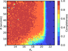 |
Fig. 1 Two-dimensional completeness map as a function of Ks magnitude and the distance R from the center of 47 Tuc. |
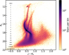 |
Fig. 2 Hess diagram in the Ks vs J − Ks color-magnitude space of all sources detected in tile SMC 5_2 based on PSF photometry. The mean photometric errors as a function of the Ks magnitude are indicated on the left-hand side as black bars. Note that the color scale is in logarithmic units. |
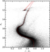 |
Fig. 3 CMD of all stars within 20′ from thecenter of 47 Tuc. The diagram is dominated by stars belonging to the cluster, but the sequences of the Milky Way and the SMC are still visible. An isochrone at 11.8 Gyr from the PARSEC model set (Bressan et al. 2012) is also shown as a red line, with Z = 0.0033, E(B − V) = 0.04 mag and |

3 Propermotion calculations
Our strategy for determining the proper motions of the stars in tile SMC 5_2 was to calculate them separately for each detector and each pointing. In this way, we minimize systematic effects that may arise when combining several detectors or pointings. For each of the 12 epochs, there are 96 individual catalogs (16 detectors, 6 pointings), resulting in 1152 catalogs in total. In addition to the name of the observation and the detector number, these catalogs contain the RA and Dec coordinates, the magnitude and its uncertainty, the sharpness and the x and y coordinates on the detector chip for each star. In the following, we outline the different steps for calculating the proper motions of the stars. The overall procedure is similar to that described by Cioni et al. (2016).
3.1 Star and galaxy catalogs
In a first step, we selected only the sources that have detections in the J and Ks filters from the deep multi-band catalog and assigned a unique identification number to each source to be able to trace them throughout the calculations. We then cross-correlated this source list with the single-epoch Ks catalogs, using the IRAF task xyxymatch with a matching radius of 0.5 arcsec. In this way, we removed spurious detections from the calculations. We also assigned the Mean Julian Date (MJD) of the respective observation to each catalog, which was extracted from the multi-epoch aperture photometry files queried from the VSA website, which have been used by Cioni et al. (2016).
In addition to the different stellar populations from the cluster itself, the Milky Way and the SMC, the catalogs also contain detections of background galaxies (see Sect. 2 and Fig. 2). The reflex proper motion of these distant background objects is assumed to be zero. We used the galaxies in a next step for an initial transformation of the various epochs to a common frame of reference. An additional, refined transformation was also performed using stars of the cluster itself. Based on several selection criteria, which we discuss below, we identified sources from the catalogs that are most likely galaxies and split our catalogs into two separate sets, one containing only stars, and the other containing only the galaxies. For each source in the deep multi-band catalog, there is a discrete stellar probability parameter that can have four values (0.0, 0.33, 0.67, and 1.0). It is calculated from the position in the color-color diagram, the local completeness, and the sharpness. We selected sources as background galaxies that are classified as stars with a probability of less than 34% and that also have J − Ks colors greater than 1.0, as well as a sharpness parameter larger than 0.3 in both filters. At a sharpness of ~0.3, the sequence of the galaxies separates from the one of the stars in a sharpness vs magnitude diagram. Blends of dwarf stars that could be misclassified as galaxies because of their shapes are expected to be bluer than J − Ks = 1.0 and are not thought to contaminate our galaxy sample by much. To obtain only well-measured galaxies, we additionally restricted our final sample to galaxies with photometric errors <0.1 mag and Ks magnitudes >15 mag, also to avoid contamination by saturated stars. Since we set a limit on the photometric error of the galaxies, we did not employ a faint limit in our galaxy selection. Using a combination of selection criteria in combination with conservative limits, we ensured that we obtained a sample of galaxies that is as clean as possible. The only potential contaminants are young stellar objects in the SMC that are expected to fall into the chosen color range and have extended emission as a result of circumstellar material. The fraction of these objects contributing to our galaxy sample is negligible (a few per cent or less), however, given the size of the field and the location at the outskirts of the SMC. We ended up with a list of about 18 100 galaxies (see Fig. 4 for a CMD illustrating the selected galaxies).
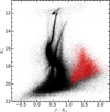 |
Fig. 4 Ks vs J − Ks CMD of unique sources detected in tile SMC 5_2. The final selected sample of background galaxies used for the transformations is shown in red. |
3.2 Common reference frame
In the next step, we transformed the catalogs from the various epochs into a common reference frame since there might be some small offsetsand/or rotations between observations at different epochs. We performed the transformation in two steps. First, we used the previously extracted galaxies, which are assumed to represent a fixed grid of non-moving points, to perform an initial transformation. Then we used stars of 47 Tuc itself for a second, refined transformation. The first step using galaxies is necessary since large initial shifts between single epochs can lead to spurious matches in the inner crowed regions of the cluster and reduce the quality of the transformation. For the cluster stars we selected only well-measured stars (photometric errors σ(Ks ) ≤ 0.05 mag, since we used only the Ks filter for the proper motion determinations) from our catalog. To obtain a clean sample of cluster stars, we minimized contamination by the otherstellar populations present in tile SMC 5_2, which are unrelated to the cluster itself (see, e.g., Fig. 2). Especiallyat fainter magnitudes, these populations overlap significantly with the 47 Tuc stars in the CMD. We therefore selected only those stars in the CMD that are brighter than the RC feature of the SMC, which lies on top of the MS of 47 Tuc at Ks ~ 17 mag. Additionally, we applied a mask in the color-magnitude space that follows the main CMD features of 47 Tuc (see Fig. 7). Our final list of cluster stars for the definition of the reference frame contains about 46 200 objects.
As our reference epoch we chose TK9, because it was observed under good conditions (see Table 1) and it includes the largest number of detected galaxies. In most of the detectors, the number of galaxies is typically between 100 and 400. However, in the detectors that image the innermost parts of 47 Tuc, the number of galaxies is reduced significantly owing to the high crowding in these regions (see Fig. 5 for the first pawprint exposure of TK9, as an example). There, we only have on the order of 30 galaxies. The opposite is true for the distribution of the cluster stars. There are several thousand stars in the detectors that cover the inner parts of the cluster, but there are only on the order of 50 stars in the detectors covering the outskirts (see middle panel of Fig. 5).
For the matching and transformation, both galaxy-based and star-based, we used the three IRAF tasks xyxymatch, geomap, and geoxytran. The first routine, xyxymatch, matches a list of input coordinates with the reference coordinate table. The task geomap usesthe matched coordinate pairs from xyxymatch as an input to compute a transformation between the input and reference system. We allowed for a general fit geometry, including a shift, rotation, and scaling, in both the x and y directions. Finally, geoxytran transforms the coordinates from the input table into the reference frame using the parameters determined by geomap. We performed this transformation procedure for each detector in all pawprints to convert them into the corresponding ones in our reference epoch TK9. Table 2 gives the statistics of the initial transformation using the galaxy frame resulting from geomap. After inspection of the quality of the conversions, we found that the r.m.s. residuals in x and y were always below 0.17 pixels, except for epoch TK5, where the r.m.s. was in general above 0.2 pixels. Cioni et al. (2016) have noted that there are some problems with this epoch, possibly due to the high airmass. They excluded it from their calculations, and we also decided not to use it for further calculations.
We then performed the refined transformation using the catalogs resulting from the initial one as the input and the cluster stars as the reference points. The statistics of this second transformation are listed in Table 3. The table shows that only small corrections are required. The r.m.s. residuals in the x and y direction are now below 0.09 pixels.
We repeated the above steps and also incorporated quadratic terms in the transformation to explore their effect on the final result. However, we found that allowing for quadratic transformations introduces additional scatter in the proper motion of both the galaxies and the stars. For this reason, we decided to use only the linear transformations.
Statistics of the results from the geomap transformation using background galaxies for the definition of the common reference frame.
Statistics of the results from the geomap transformation using the stars of the cluster itself for the definition of the common reference frame.
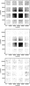 |
Fig. 5 Top panel: positions on the detectors of all stars detected in the first pawprint observation for our reference epoch TK9. For demonstration purposes, the detectors are shifted by fixed offsets in the x and y directions and the gaps between them do not reflect the real gaps between the different detectors. For this reason, the cluster appears slightly elongated in this image. In this plot, detector 1 is in the lower left corner and detector 16 is in the upper right corner. The detector numbers increase from left to right and from bottom to top. The x -axis extends approximately along the Dec direction, and the y-axis extends approximately along the RA direction. Middle panel: same as the top panel, but for the cluster stars. Bottom panel: same as the top panel, but for the galaxies. |
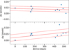 |
Fig. 6 Position of a single random star on one detector chip as a function of time (filled circles). The solid line is the best-fitting linear curve to the data. The dashed lines indicate the 1σ distance of the stars from the fitted line. The zero-point of the ordinate is arbitrarily chosen with respect to the minimum value. |
3.3 Deriving the proper motions
After the preparatory work described in the previous sections, our final data set for the computation of the proper motions consisted of catalogs at 11 different epochs, all shifted to a common frame of reference. We separately identified for all detectors and pawprints all stars that are detected in all epochs (about 60% of the total number of stars) and created catalogs for each star, containing the various x and y positions on the detector chip and the respective MJDs. Next, we fit a linear least-squares regression model independently to the x and y values as a function of the MJD. Figure 6 shows the x and y measurements of a random star in our sample on a single detector at the various epochs as an example, together with the best-fitting linear model. The slope of the fitted model gives us the proper motions dx and dy of the sources in units of pixels day−1.
Finally, we transformed the results into a more meaningful physical unit. For this, we first applied the following transformation equations to our values (see also Cioni et al. 2016), which take into account the pixel scale and the rotation of the detector with respect to the sky coordinates:

We followed the convention introduced by Cioni et al. (2016), where dξ equals μα cos(δ) and dη stands for μδ with α running along the right ascension and δ along the declination axes. The four coefficients CD1,1, CD1,2, CD2,1 , and CD2,2 are the transformation matrix elements that account for the rotation of the field on the plane of the sky and for the pixel scale. They can be retrieved from the FITS headers of the detectors of all pawprints of the reference epoch. We note that the astrometry of VISTA pawprints shows a systematic pattern on the order of 10–20 mas coming from residual World Coordinate System (WCS) errors6 . This effect limits the precision of the proper motion measurements of single objects in this study. We show below (see Sect. 4.2.2), however, that our overall results are in good agreement with recent studies, which suggests that there is no significant systematic offset in the astrometry. We expect the precision of the VISTA astrometric solution to improve in the future since it will be calibrated using Gaia DR2 data.
The above equations transform our proper motion measurements from pixels day−1 into deg day−1, which we finally converted into mas yr−1. We also applied the same method to our sample of galaxies. We use the reflex proper motions of the galaxies as our zero-point below to determine the motions of the stars.
Our final star catalog of proper motions includes a total of 277 908 objects. The positions of the six pawprint pointings are designed to ensure that the resultingtile automatically observes each object in at least two different pawprints (except in narrow strips at the outside edge of the tiles). A small fraction of objects will be observed more than twice, along edges and corners of detectors. Thus roughly half of the objects in the six pawprints that make up a tile correspond to the same object on the sky, although some objects will appear more than twice. In total, there are 134 605 unique entries in our catalog of stars. The derived proper motions of all stars in this tile are absolute proper motions, since they have been calculated with respect to background galaxies, which represent a non-moving reference frame. We will make the proper motion catalogs publicly available upon request.
4 Results and analysis
4.1 The proper motion of 47 Tuc
4.1.1 The VMC survey data
For the calculation of the median proper motion of 47 Tuc, we applied the same criteria as in Sect. 3.2 to select the cluster members. Owing to high crowding in the innermost parts of the cluster, our results suffer from inaccurate measurements of the stellar centroids, even when using PSF photometry. We therefore excluded the inner 5′ of the cluster from further calculations. Furthermore, we restricted our final sample to stars that are within the cluster tidal radius of ~42′ (we assumed the same value as Cioni et al. 2016). We were left with a total of 78 535 detections of potential cluster members (34 877 unique stars, considering the multiple detections) to calculate the proper motion of the cluster. After the star-based transformation, the cluster stars are at rest, whereas the galaxies move. The proper motion of the cluster with respect to the galaxies is therefore given by the negative median reflex motion of the background galaxies. We found a median proper motion of 47 Tuc of (μα cos(δ), μδ) = (+5.89, −2.14) mas yr−1 with a statistical error of 0.02 mas yr−1 in both directions. These values have been corrected for the median residual motions of the cluster stars in the α and δ direction (dξ = 0.00 ± 0.02 and dη = 0.07 ± 0.02 mas yr−1) to place them at rest. The statistical error of the measurements is calculated as the median absolute deviation (MAD) divided by the square root of the numbers of stars. The MAD is defined as the median of the difference between the measurements and its median. Owing to the large numbers of stars used to calculate the absolute proper motion of 47 Tuc, the statistical error is very small.
In addition to the statistical error, there are also systematic uncertainties, which are mostly caused by atmospheric turbulence, the uncertainties in the calibration of the individual detector images using 2MASS stars, and the atmospheric differential refraction. To limit the effects of this last contribution, we used only observations in the Ks band taken at similar air masses for our calculations (the epoch with the highest air mass was removed because of high residuals in the transformation). For a detailed discussion of the various sources of errors, see Cioni et al. (2016). We can estimate the systematics from the uncertainties in the cluster star based reference frame. Looking at the proper motions of the stars as a function of detector number (see Fig. A.1), we found a scatter of the median motion of 0.50 mas yr−1 in the RA direction and 0.31 mas yr−1 in the Dec direction, resulting in a larger uncertainty in the first direction. A good measure of the statistical uncertainties of the proper motions results would be the scatter of the median proper motions of the stars scaled to the square root of the number of the detectors. This results in an error of 0.13 mas yr−1 in the RA direction and 0.11 mas yr−1 in the Dec direction, also taking the residual motion of the stars in the Dec direction into account. This demonstrates that the precision of the measurements is limited by the systematic uncertainties. Our final result of the absolute proper motion of 47 Tuc is (μα cos(δ), μδ) = (+5.89 ± 0.02 (statistical) ± 0.13 (systematic), −2.14 ± 0.02 (statistical) ± 0.08 (systematic)) mas yr−1. The optical desing of VISTA results in a radially symmetric cubic (pincushion) scale distortion at the VIRCAM detectors, which in turn results in a smaller pixel size at the edges of a pawprint (see Sutherland et al. 2015). The maximum difference in pixel scale between the central parts and the outermost parts in the pawprint is on the order of 2 percent, which translates into a difference in proper motion of 2 percent as well. Since the mean variation in pixel size is much smaller and we averaged the results from many stars spread over a large area within the pawprint for our analysis, we can neglect the effect of the distortion here.
We also studied the results of the proper motion of 47 Tuc when only the galaxy-based transformation into a common frame of reference was used. In this case, the galaxies are at rest and the stars of the clusters move, and for the median proper motion of 47 Tuc, we found (μα cos(δ), μδ) = (+5.44 ± 0.02 (statistical) ± 0.15 (systematic), −2.52 ± 0.02 (statistical) ± 0.28 (systematic)) mas yr−1. To put the galaxies at rest, these values were corrected for the median residual reflex motion of the galaxies in the α and δ direction (dξ = −0.12 ± 0.12 and dη = 0.01 ± 0.12 mas yr−1). When we compare the galaxy-based measurement of the proper motion of 47 Tuc with the star-based value, we can see that both components of the former are smaller. In the Dec direction, the difference is somewhat larger than the 1σ uncertainty, whereas the two values differ by about 2.3σ in the RA direction. The number of reference objects to calculate the relative proper motion is significantly different in the two methods. This allows for a more well-defined reference system in the star-based method and results in a final value that differs moderately from the galaxy-based value. We show in Sect. 4.2.2 that the values from both methods are compatible with the range of results from recent studies.
Next, we explored how stable our result is with respect to the size of the sample of stars used. This will help us to assess the reliability ofour measurements in regions where fewer stars are available. For this, we created 70 000 (approximate number of stars in our original sample) sub-samples of stars from our original cluster catalog. Each consisted of a random number of stars that were drawn randomly from the original list of cluster stars. We then calculated the median proper motion of every sub-sample. The results are shown in Fig. 8. Each point represents an individual measurement and is color-coded by the number of stars used. The black cross marks the proper motion value that is derived from the entire list of cluster stars. As expected, the fewer stars used for the calculation, the less accurate the result. Especially for sample sizes of less than a few hundred stars, the original signal imprinted in the data is lost in the measurement errors of the individual stars, and the final result becomes more or less random. To quantify the reliability of the results using variable numbers of stars, we calculated the medians and standard deviations of all values in bins of 500 stars (see Fig. 9). For a sample size of 2000 stars, the 1σ scatter is on the order of 0.3–0.4 mas yr−1 around the original value. This scatter decreases to about 0.1 mas yr−1 for catalogs of 10 000 stars. From this test, we conclude that for a reasonable and reliable result, we need sample sizes of at least 1500–2000 stars.
Finally, we examined the reflex proper motions of the background galaxies and the proper motions of the cluster stars as a function both of the J − Ks color and the distance to the center of 47 Tuc to look for any systematic trends in the motion of these objects. The corresponding figures are presented in the appendix (Figs. A.2 and A.3) and show the distributions of the individual proper motions together with the running mean. In almost all cases, we do not find any significant trend of the proper motions as a function of the color or distance from the cluster center. The only exception where a trend might be present is the Dec component of the galaxies’ reflex motion as a function of the distance from the cluster center (see top right panel of Fig. A.3). There, the mean reflex motion is systematically below zero at radii smaller than ~33′ and above zero at larger radii. A Spearman correlation test reveals that in this case, the correlation coefficient is about 0.02, whereas in the other cases, it is always well below 0.01. Since we are only interested in the overall movement of 47 Tuc and the median reflex motion of the galaxies across all detectors is close to zero (dη = 0.01 ± 0.12 mas yr−1), this slight trend has no significant effect on our final results.
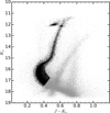 |
Fig. 7 CMD of all stars with Ks photometric errors σ(Ks) ≤ 0.05 mag. The stars we selected for our calculation of the proper motion of 47 Tuc are highlighted as black dots. |
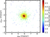 |
Fig. 8 Resulting proper motion values of 47 Tuc when choosing a randomly selected sub-sample of cluster stars. Each point represents an individual result and is color-coded by the number of stars used for the calculation. The “real” value using all stars is indicated by the black cross. |
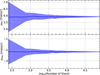 |
Fig. 9 Median value of the sub-sample results shown in Fig. 8 in bins of 500 stars (solid blue line), along with its standard deviation (blue shaded area). The bottom panel shows the proper motion in the Dec direction, and the top panel shows the proper motion in the RA direction. |
4.1.2 The UCAC5 Catalog
In addition to the VMC result, we also used data from the newest US Naval Observatory CCD Astrograph Catalog (UCAC5) proper motion catalog, which also includes data from Gaia DR1 (Zacharias et al. 2017) for an independent measurement of the proper motion of 47 Tuc. From the catalog7 , we queried all stars that reside within 42′ of the cluster center. Similarly to the VMC data, we masked the main CMD features of the cluster to obtain a cleaner sample of cluster stars. We selected stars that follow the RGB, RC, and asymptotic giant branch of 47 Tuc. Additionally, we limited our sample to stars with magnitudes brighter than 14.0 in the Ks band, whichis about one magnitude above the sensitivity limit of the data. Our final list contains about 2750 stars. The top panel of Fig. 10 shows the spatial distribution of the queried stars. The black dots indicate the stars we selected for our proper motion calculation. The bottom panel of Fig. 10 shows the same stars in a CMD using the 2MASS J and Ks filters. Again, the selected stars are denoted by black dots. Using this final list of stars, we found a median proper motion of the stars in 47 Tuc of (μα cos(δ), μδ) = (+5.30, −2.70) mas yr−1 with a statistical error of 0.03 mas yr−1 in both directions. The precision, in terms of the statistical uncertainties, of this measurement is comparable to the one from the VMC data, although we calculated the proper motion from a much smaller number of stars using the UCAC5 catalog. The reason for this is that the proper motions in the UCAC5 catalog are calculated using a much longer time-baseline ( ~14 years). However, Zacharias et al. (2017) noted that the proper motions suffer from systematic uncertainties, which can be as large as 0.7 mas yr−1. The final result of the proper motion of 47 Tuc from the UCAC5 data catalog is (μα cos(δ), μδ) = (+5.30 ± 0.03 (statistical) ± 0.70 (systematic), −2.70 ± 0.03 (statistical) ± 0.70 (systematic)) mas yr−1, which agrees with the value from the VMC data within the uncertainties. The UCAC5 catalog would be only suitable for limited dynamical studies of the Magellanic Clouds. Since its sensitivity limit is at Ks ~ 15 mag (the RC of the SMC is more than 2 magnitudes fainter, see Fig. 2), it reaches only the brightest evolved stars (upper RGB, AGB) in the Clouds.
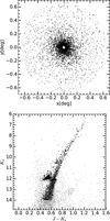 |
Fig. 10 Top panel: spatial distribution of stars in the UCAC5 catalog within 42′ of the center of 47 Tuc. Stars selected for the proper motion calculation are indicated by black dots. Bottom panel: Ks vs J − Ks CMD of thestars shown in the top panel. |
4.2 Comparison with literature values
4.2.1 Results from aperture photometry
Cioni et al. (2016) have calculated the proper motion of the different stellar populations present in VMC tile SMC 5_2, including 47 Tuc, using aperture photometry measurements. For the cluster, they found (μαcos(δ), μδ) = (+7.26 ± 0.03 (statistical) ± 0.18(systematic), −1.25 ± 0.03(statistical) ± 0.18 (systematic)) mas yr−1. This is incompatible with the values found in this work using PSF photometry. When using the star-based transformation, the difference in μαcos(δ) is 6.2σ and in μδ it is 4.5σ . When using the galaxies as the frame of reference, the results differ by 8σ in μαcos(δ) and in μδ by 4σ. In the following we discuss several reasons that might be responsible for this discrepancy. We base our discussion here on our result from the galaxy-based transformation, since Cioni et al. (2016) also used the galaxies as their reference points.
As a first point, the different time-baseline used to calculate the proper motions is to be mentioned. Cioni et al. (2016) only used the deep exposures, which span in total about 12 months. In our study, we also included the first shallow epoch, which extends the time baseline to about 17 months. To assess the effect of the longer time interval, we recalculated the proper motions using only the 10 deep observations, which yields (μαcos(δ), μδ) = (+5.43, −1.41) mas yr−1. The shorter time-baseline shifts our result closer to the one obtained by Cioni et al. (2016) in the Dec direction, but there is only a slight change in the RA direction.
Second, the selection of the stars used to calculate the absolute motion of 47 Tuc is different in the two studies. For their calculations, Cioni et al. (2016) used all stars between 10′ and 60′ from the center of the cluster that are within certain CMD regions (see their Fig. 6), which results in approximately 70 000 measurements in total. To compare the effect of the different stellar samples, we applied the same selection criteria to both proper motion catalogs. When we applied the same radial range and CMD region masks as Cioni et al. (2016) to our data using our original set of epochs, we found (μα cos(δ), μδ) = (+4.64, −2.61) mas yr−1. With the shorter time-baseline, the proper motion now becomes (μα cos(δ), μδ) = (+4.38, −1.50) mas yr−1. This value is now lower than our original result, most likely because the new sample also includes RC stars from the SMC, which have smaller proper motions. We also applied our selection of 47 Tuc stars to the Cioni et al. (2016) catalog, which gives (μα cos(δ), μδ) = (+7.06, −1.36) mas yr−1. The various selections of stars change the overall result but cannot account for the entire difference of the outcomes of the two methods, which suggests an intrinsic difference in the two catalogs.
The third reason is the different determination of the stellar centroids in the standard VDFS pipeline and the PSF-fitting technique, which becomes especially evident in regions with a high stellar density, like in the inner part of the cluster. We cross-correlated single-epoch PSF and aperture photometry stellar catalogs of various detectors to quantify the differences in stellar positions resulting from the two methods. We found that regardless of stellar crowding, there are systematic shifts both in the x and y directions of the stellar positions within a single detector. These shifts are different at different epochs and usually vary between 0 pixels and (1− 2) × 10−2 pixels, but there are also single cases where the shifts are as large as ~ 5 × 10−2 pixels. The differences in stellar positions in both directions have a 1σ scatter, which is about 0.2 pixels in crowded regions and ~0.06 pixels in less crowded regions. We also compared the proper motion results from the two methods in regions with a low stellar density. For this, we selected stars with distances larger than 40′ from the center of 47 Tuc and chose the same CMD region masks as Cioni et al. (2016) to select SMC stars along the RGB and RC. Again, using only the 10 deep observations, we found a proper motion of the SMC stars of (μα cos(δ), μδ) = (+1.23, −0.61) mas yr−1 with a statistical uncertainty of 0.07 mas yr−1. This is similar to the results by Cioni et al. (2016), who found (μα cos(δ), μδ) = (+1.16, −0.81) mas yr−1, which suggests that both methods work similarly well in less crowed regions.
Finally, Cioni et al. (2016) used a different set of galaxies for the alignment of the observations at different epochs. We have chosen our sample of galaxies by applying stricter selection criteria and have a smaller galaxy sample size. This can result in a different transformation of the various observations. As a consequence, the residual motions of the galaxies, which are subtracted from the proper motions of the stars, are not the same. The resulting reflex proper motion of the galaxies in Cioni et al. (2016) was (μα cos(δ), μδ) = (−0.45 ± 0.12, −0.15 ± 0.12) mas yr−1, whereas in this work, it was (μα cos(δ), μδ) = (−0.12 ± 0.12, 0.01 ± 0.12) mas yr−1.
4.2.2 Other results from the literature
In this section we compare our results with other proper motion measurements from the literature. The most recent one has been presented by Narloch et al. (2017), who used data from the 1m Swope telescope of the Las Campanas observatory. They calculated the mean proper motion of 47 Tuc with respect to the motion of the SMC using two different fields with time baselines of ~11 and ~17 years, respectively. Adopting a mean value for the motion of the SMC from various measurements in the literature, the authors found for the absolute proper motion of the cluster (μα cos(δ), μδ) = (+5.376 ± 0.032, −2.216 ± 0.028) mas yr−1. Their valueagrees with our measurement within the 1σ uncertainties in the Dec direction, but is higherby about 3.8σ in the RA direction.
Watkins & van der Marel (2017) used data from the TGAS catalog to study the motion and distances of a sample of five globular clusters. They calculated the weighted mean of five identified member stars of 47 Tuc from the TGAS catalog and found as a result (μαcos(δ), μδ) = (+5.50 ± 0.70, −3.99 ± 0.55) mas yr−1. The authors state that the uncertainties in their measurements are dominated by random errors and the systematic errors are much smaller than those. Our result for the cluster motion is consistent with the finding of Watkins & van der Marel (2017) in the RA direction within the errors. However, in the Dec direction, the results disagree by about 3.3σ. This discrepancy might be due to selection effects since the measurement in Watkins & van der Marel (2017) results from only five cluster stars.
Freire et al. (2003) and in a follow-up study, Freire et al. (2017), observed millisecond pulsars within 47 Tuc. From a weighted average of the proper motions of these pulsars, the authors determined the motion of the cluster in their first paper as (μαcos(δ), μδ) = (5.3 ± 0.6, −3.3 ± 0.6) mas yr−1. In the second paper, where the long-term observations of the pulsars are presented, Freire et al. (2017) found (μαcos(δ), μδ) = (5.00 ± 0.14, −2.84 ± 0.12) mas yr−1 for the proper motion of the cluster. In the RA direction, the older measurement is in agreement with our result, whereas the updated value found by Freire et al. (2017) is about 4.6σ away. In the Dec direction, both values from Freire et al. are lower than ours. They differ by about 1.9σ (Freire et al. 2003) and 4.9σ (Freire et al. 2017).
Anderson & King (2003) used observations taken with the Hubble Space Telescope (HST) to derive the proper motion of 47 Tuc. They used two different fields across the cluster, each of which was observed twice, with a time baseline of five and six years, respectively. As a reference frame, they used the background stars of the SMC, so that the resulting proper motion of the cluster depends on the assumed value for the motion of the SMC. Anderson & King (2003) found a motion of the SMC with respect to 47 Tuc of (μα cos(δ), μδ) = (−4.716 ± 0.035, +1.357 ± 0.021) mas yr−1. For the motion of the SMC, they took the results from Irwin (1999), who gives (μα cos(δ), μδ) = (0.92 ± 0.20, −0.69 ± 0.20) mas yr−1. This results in an absolute proper motion of 47 Tuc of (μα cos(δ), μδ) = (5.64 ± 0.20, −2.05 ± 0.20) mas yr−1. Combining the results of Anderson & King (2003) with more recent measurements of the motion of the SMC from Kallivayalil et al. (2006) or Cioni et al. (2016) gives (μα cos(δ), μδ) = (5.88 ± 0.20, −2.53 ± 0.20) mas yr−1 (Kallivayalil et al. 2006) and (μα cos(δ), μδ) = (5.88 ± 0.20, −2.17 ± 0.20) mas yr−1 (Cioni et al. 2016), respectively. When the updated values for the SMC motion are used, the result in the RA direction from Anderson & King (2003) is in very good agreement with our measurement. In the Dec direction, both values are also consistent using the SMC motion from Cioni et al. (2016), but they differ by 1.9σ assuming the value from Kallivayalil et al. (2006).
Odenkirchen et al. (1997) used data from the hipparcos mission to measure the proper motions of 15 globular clusters, including 47 Tuc, for which they found (μα cos(δ), μδ) = (7.0 ± 1.0, −5.3 ± 1.0) mas yr−1. They estimated the error in the absolute proper motion from the dispersion of the proper motions of cluster stars and the accuracy of the hipparcos reference frame. In the RA direction, the value obtained by Odenkirchen et al. (1997) is higher than ours and just outside the 1σ uncertainty. In the Dec direction, our measurement is larger by about 3.2σ.
Cudworth & Hanson (1993) found a proper motion of 47 Tuc of (μα cos(δ), μδ) = (3.4 ± 1.7, −1.9 ± 1.5) mas yr−1 when converting the relative motion of the cluster with respect to background stars into an absolute proper motion, where the given error is the combined error of the cluster relative proper motion uncertainty and the error of the proper motion of the reference stars. Our result agrees with the one found by Cudworth & Hanson (1993) within the 1σ uncertainty in the Dec direction and is largerby about 1.5σ in the RA direction.
The different measurements, together with the results obtained in this paper, are summarized in Table 4 and also illustrated in Fig. 11. Our measurement is closest to the results obtained by Narloch et al. (2017) and Anderson & King (2003). Additionally, our values for the motion in the RA direction agree very well with those obtained by Freire et al. (2003) and Watkins & van der Marel (2017), although our value in the Dec direction is higher than theirs.
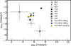 |
Fig. 11 Comparison of the median proper motions presented in this paper with values from the literature. Where nouncertainty is shown, it is smaller than the size of the symbol. The abbreviations in the legend are the following: N17: Narloch et al. (2017); F17: Freire et al. (2017); W17: Watkins & van der Marel (2017); C16: Cioni et al. (2016); A03: Anderson & King (2003), using the SMC motion from Kallivayalil et al. (2006); F03: Freire et al. (2003); O97: Odenkirchen et al. (1997); C93: Cudworth & Hanson (1993). VMCg : from the VMC data using a galaxy-based reference frame for the transformations between single epochs; VMCs : from the VMC data using a star-based reference frame for the transformations between single epochs; UCAC5: from the UCAC5 catalog. |
Proper motion measurements of 47 Tuc from the literature.
4.3 Orbit of 47 Tuc
In this section, we examine the orbit of 47 Tuc within the Milky Way in more detail. For this, we combine the cluster proper motion derived in this work with radial velocity measurements from the literature to obtain the full 3D velocity vector of the cluster. Marino et al. (2016) performed a chemical abundance analysis of a sample of 75 RGB stars in 47 Tuc, thereby also deriving the radial velocity of the stars. They found a mean radial velocity of − 16.73 ± 0.77 km s−1 with an r.m.s. of 6.66 km s−1. We used this value for our analysis. For the spatial position of the cluster, we adopted the center of 47 Tuc as derived in Li et al. (2014) ( , δ2000 = −72°04′48″) and the distance of 4.57 kpc, resulting from our isochrone match to the data (see Sect. 2). For the modeling of the cluster orbit, we made use of the python package galpy8 (Bovy 2015). We assumed a Milky Way-like potential, called MWPotential2014, which is composed of three components, an exponentially cutoff power-law density bulge, a Miyamoto-Nagai disk, and a dark matter halo as described in Navarro et al. (1997). The galpy package accepts the observed quantities of the velocity and position as input values and converts them into the corresponding values in the Galactic frame. We integrated the orbit backward for 12 Gyr (the approximate age of the cluster). The orbit integration assumes a static potential that does not change over the time of integration. This is just an approximation, however, since the Milky Way most likely has merged with a number of small galaxies in the past. For this reason, the orbit of the cluster becomes less reliable in the later stages of the simulation. Figure 12 shows the resulting orbit in the Galactocentric R vs z plane, with the current position of the cluster indicated as a red filled circle and the direction of the present-day motion illustrated by the black arrow. The resulting ellipticity of the orbit is e ~ 0.2. The pericenter and apocenter are at radii of ~5.1 kpc and ~7.5 kpc, respectively, whereas the maximum height above and below the Galactic plane is ~3.6 kpc. According to our simulation, the cluster is confined within the inner regions of the Galaxy.
Our results are in line with the findings of Odenkirchen et al. (1997) and O’Malley et al. (2017). In their study, Odenkirchen et al. (1997) derived the proper motions of a sample of 15 Galactic globular clusters from hipparcos data and combined their results with quantities from the Harris (1996) catalog to determine the overall motions of the clusters. For the calculation of the orbital parameters, they used a three-component potential. Odenkirchen et al. (1997) found for 47 Tuc an orbit that extends between 4.3 and 7.9 kpc from the Galactic Center with a maximum height above the Galactic plane of 4.3 kpc. Additionally, they found an orbit ellipticity of 0.30. Recently, O’Malley et al. (2017) analyzed the orbits of a sample of 22 clusters, including 47 Tuc. They used an average of the Anderson & King (2003) and Freire et al. (2003) results for the proper motions, and for the line-of-sight velocity and the position and distance, they used the entries in the Harris (1996) catalog (2010 edition). O’Malley et al. (2017) found the 47 Tuc orbit to be within 8 kpc from the Galactic Center with a maximum vertical height of 4 kpc and an ellipticity of 0.21 (see their Fig. 4). The similarity of the results from these studies indicates that the orbital parameters are quite robust to moderate changes in the phase-space parameters of the cluster.
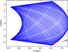 |
Fig. 12 Orbit of 47 Tuc in the Galactocentric R vs z plane. The orbit has been integrated back to 12 Gyr ago. The current position of the cluster is indicated by the red filled circle, and the direction of the present-day motion is represented by the black arrow. |
5 Conclusions
We used multi-epoch observations from the VMC survey to derive the proper motions of stars within the globular cluster 47 Tuc. Taking advantage of the improved stellar position determinations from PSF photometry and an increased time baseline, we found a median proper motion of the cluster of (μα cos(δ), μδ) = (+5.89 ± 0.02 (statistical) ± 0.13 (systematic), −2.14 ± 0.02 (statistical) ± 0.11 (systematic)) mas yr−1. We also calculated the absolute proper motion of the cluster using data from the UCAC5 catalog. There we found (μα cos(δ), μδ) = (+5.30 ± 0.03 (statistical) ± 0.70 (systematic), −2.70 ± 0.03 (statistical) ± 0.70(systematic)) mas yr−1, which agreeswith the results from the VMC data within the uncertainties. Combining our results with radial velocity measurements from the literature, we were able to reconstruct the cluster orbit for its current lifetime ( ~12 Gyr), showing that 47 Tuc was confined within the inner ~7.5 kpc of the MilkyWay with a maximum vertical distance from the Galactic plane of about 3.6 kpc.
When comparing our results for the proper motion with various previous determinations from the literature, we found that both the VMC valuesare closest to the measurements from Narloch et al. (2017), and Anderson & King (2003) (using updated proper motions for the SMC). However, our results differ from those presented by Cioni et al. (2016), using stellar positions from the VDFS pipeline, by 8σ in μαcos(δ) and 4σ in μδ . We identified the longer time-span between the observations as well as the differences in the stellar centers, especially in the most crowded regions, as the main sources that lead to this discrepancy. We showed that the technique we presented for deriving proper motions using data from the VMC survey works very well for our test case of 47 Tuc with the improvements we described.
In upcoming studies we will use the wealth of VMC data and apply the techniques we developed and described in this preparatory work to study the overall and internal kinematics of the SMC. The VMC survey is designed such that on average, all tiles have a time baseline of about two years for the multi-epoch Ks observations. We will thereby concentrate on the SMC-Bridge region, where Subramanian et al. (2017) found large differences in the line-of-sight distance of the stars, but also on the kinematics of the different stellar populations that are shown to have large spatial differences within the galaxy (e.g., Ripepi et al. 2017). Adding a kinematic component to these observations will help us to better understand the history of the Magellanic System.
Acknowledgements
We thank the Cambridge Astronomy Survey Unit (CASU) and the Wide Field Astronomy Unit (WFAU) in Edinburgh for providing calibrated data products under the support of the Science and Technology Facility Council (STFC). This project has received funding from the European Research Council (ERC) under European Union’s Horizon 2020 research and innovation programme (grant agreement No 682115). R. d. G. is grateful for research support from the National Natural Science Foundation of China (NSFC) through grants 11373010, 11633005, and U1631102. This research made use of Astropy, a community-developed core Python package for Astronomy (Astropy Collaboration et al. 2013). This study is based on observations obtained with VISTA at the Paranal Observatory under program ID 179.B-2003. We thank the anonymous referee for useful comments and suggestions that helped to improve the paper.
Appendix A: Proper motion trends
In the appendix we present additional plots to search for any trends of the proper motion as a function of different quantities. All figures showthe reflex proper motions of galaxies and the proper motions of the cluster stars separately. For the galaxies, the reflex proper motion is calculated after the galaxy-based initial transformation, and for the cluster stars, the proper motion is determined after the refined transformation to a common reference frame using the cluster stars itself. Therefore, it is expected that the proper motions have a mean value of zero for both types of sources (indicated by a dashed line in each panel).
The top panels of Fig. A.1 show the median reflex proper motions of the galaxies on each detector. The error bars indicate the median absolute deviation (MAD) divided by the square root of the number of galaxies within each detector. The bottom panels show the same for the proper motion of the cluster stars.
The top panels of Fig. A.2 show the individual reflex proper motions in both directions of the galaxies as a function of the J − Ks color. The red solid line indicates the running mean of all sources. The bottom panels show the same for the proper motions of the cluster stars. For both types of sources, no trends of the proper motions with color are found.
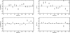 |
Fig. A.1 Toppanels: median reflex proper motions of galaxies in mas yr−1 on each detector. The error bars are the MAD divided by the square root of the number of galaxies within each detector. The left-hand panel shows the proper motions in the RA direction, whereas the right-hand panel is for the Dec direction. Bottom panels: same as the top panels, but now for the proper motions of the cluster stars. |
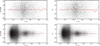 |
Fig. A.2 Toppanels: individual reflex proper motion values of galaxies in mas yr−1 as a functionof the J − Ks color. The running mean of this distribution is shown as the red solid line. The left-hand panel shows the proper motion in the RA direction, whereas the right-hand panel is for the Dec direction. Bottom panels: same as the top panels, but now for the proper motions of the cluster stars. |
Figure A.3 is similar to Fig. A.2, but now the proper motions as a function of the distance from the center of 47 Tuc are shown. There might be a slight trend of the galaxies’ reflex motion as a function of the distance to the cluster center. In all other cases, there are no obvious trends seen in the proper motion.
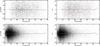 |
Fig. A.3 Toppanels: reflex proper motions of individual galaxies in mas yr−1 as a function of the distance in arcmin to the center of 47 Tuc. The red solid line marks the running mean of the distribution. The left-hand panel shows the proper motion in the RA direction, whereas the right-hand panel is for the Dec direction. Bottom panels: same as the top panels but now for the proper motions of the cluster stars. |
References
- Anderson, J., & King, I. R. 2003, AJ, 126, 772 [NASA ADS] [CrossRef] [Google Scholar]
- Anderson, J., & van der Marel, R. P. 2010, ApJ, 710, 1032 [NASA ADS] [CrossRef] [Google Scholar]
- Astropy Collaboration, Robitaille, T. P., Tollerud, E. J et al. 2013, A&A, 558, A33 [NASA ADS] [CrossRef] [EDP Sciences] [Google Scholar]
- Bedin, L. R., Piotto, G., King, I. R., & Anderson, J. 2003, AJ, 126, 247 [NASA ADS] [CrossRef] [Google Scholar]
- Bellini, A., Bedin, L. R., Pichardo, B., et al. 2010, A&A, 513, A51 [NASA ADS] [CrossRef] [EDP Sciences] [Google Scholar]
- Bellini, A., Anderson, J., van der Marel, R. P., et al. 2014, ApJ, 797, 115 [NASA ADS] [CrossRef] [Google Scholar]
- Bellini, A., Bianchini, P., Varri, A. L., et al. 2017, ApJ, 844, 167 [NASA ADS] [CrossRef] [Google Scholar]
- Bogdanov, S., Heinke, C. O., Özel, F., & Güver, T. 2016, ApJ, 831, 184 [NASA ADS] [CrossRef] [Google Scholar]
- Bovy, J. 2015, ApJS, 216, 29 [NASA ADS] [CrossRef] [Google Scholar]
- Bressan, A., Marigo, P., Girardi, L., et al. 2012, MNRAS, 427, 127 [NASA ADS] [CrossRef] [Google Scholar]
- Brogaard, K., VandenBerg, D. A., Bedin, L. R., et al. 2017, MNRAS, 468, 645 [NASA ADS] [CrossRef] [Google Scholar]
- Cadelano, M., Dalessandro, E., Ferraro, F. R., et al. 2017, ApJ, 836, 170 [NASA ADS] [CrossRef] [Google Scholar]
- Cardelli, J. A., Clayton, G. C., & Mathis, J. S. 1989, ApJ, 345, 245 [NASA ADS] [CrossRef] [Google Scholar]
- Carretta, E., Bragaglia, A., Gratton, R., D’Orazi, V., & Lucatello, S. 2009, A&A, 508, 695 [NASA ADS] [CrossRef] [EDP Sciences] [Google Scholar]
- Casetti-Dinescu, D. I., Girard, T. M., Herrera, D., et al. 2007, AJ, 134, 195 [NASA ADS] [CrossRef] [Google Scholar]
- Casetti-Dinescu, D. I., Girard, T. M., Korchagin, V. I., van Altena, W. F., & López, C. E. 2010, AJ, 140, 1282 [NASA ADS] [CrossRef] [Google Scholar]
- Casetti-Dinescu, D. I., Girard, T. M., Jílková, L., et al. 2013, AJ, 146, 33 [NASA ADS] [CrossRef] [Google Scholar]
- Chatzopoulos, S., Fritz, T. K., Gerhard, O., et al. 2015, MNRAS, 447, 948 [NASA ADS] [CrossRef] [Google Scholar]
- Cioni, M.-R. L., Clementini, G., Girardi, L., et al. 2011, A&A, 527, A116 [NASA ADS] [CrossRef] [EDP Sciences] [Google Scholar]
- Cioni, M.-R. L., Girardi, L., Moretti, M. I., et al. 2014, A&A, 562, A32 [NASA ADS] [CrossRef] [EDP Sciences] [Google Scholar]
- Cioni, M.-R. L., Bekki, K., Girardi, L., et al. 2016, A&A, 586, A77 [NASA ADS] [CrossRef] [EDP Sciences] [Google Scholar]
- Costa, E., Méndez, R. A., Pedreros, M. H., et al. 2009, AJ, 137, 4339 [NASA ADS] [CrossRef] [Google Scholar]
- Costa, E., Méndez, R. A., Pedreros, M. H., et al. 2011, AJ, 141, 136 [NASA ADS] [CrossRef] [Google Scholar]
- Cross, N. J. G., Collins, R. S., Mann, R. G., et al. 2012, A&A, 548, A119 [NASA ADS] [CrossRef] [EDP Sciences] [Google Scholar]
- Cudworth, K. M., & Hanson, R. B. 1993, AJ, 105, 168 [NASA ADS] [CrossRef] [Google Scholar]
- Dalton, G. B., Caldwell, M., Ward, A. K., et al. 2006, in Ground-based and Airborne Instrumentation for Astronomy, Proc. SPIE, 6269, 62690X [CrossRef] [Google Scholar]
- D’Onghia, E., & Fox, A. J. 2016, ARA&A, 54, 363 [NASA ADS] [CrossRef] [Google Scholar]
- Emerson, J., & Sutherland, W. 2010, The Messenger, 139, 2 [NASA ADS] [Google Scholar]
- Emerson, J., McPherson, A., & Sutherland, W. 2006, The Messenger, 126, 41 [NASA ADS] [Google Scholar]
- Freire, P. C., Camilo, F., Kramer, M., et al. 2003, MNRAS, 340, 1359 [NASA ADS] [CrossRef] [Google Scholar]
- Freire, P. C. C., Ridolfi, A., Kramer, M., et al. 2017, MNRAS, 471, 857 [NASA ADS] [CrossRef] [Google Scholar]
- Gaia Collaboration (Brown, A. G. A., et al.) 2016, A&A, 595, A2 [NASA ADS] [CrossRef] [EDP Sciences] [Google Scholar]
- Harris, W. E. 1996, AJ, 112, 1487 [NASA ADS] [CrossRef] [Google Scholar]
- Høg, E., Fabricius, C., Makarov, V. V., et al. 2000, A&A, 355, L27 [Google Scholar]
- Irwin, M. 1999, in The Stellar Content of Local Group Galaxies, eds. P. Whitelock, & R. Cannon, (San Francisco: ASP), Proc. IAU Symp., 192, 409 [NASA ADS] [Google Scholar]
- Irwin, M. J., Lewis, J., Hodgkin, S., et al. 2004, in Optimizing Scientific Return for Astronomy through Information Technologies, eds. P. J. Quinn, & A. Bridger, Proc. SPIE, 5493, 411 [NASA ADS] [CrossRef] [Google Scholar]
- Kallivayalil, N., van der Marel, R. P., & Alcock, C. 2006, ApJ, 652, 1213 [NASA ADS] [CrossRef] [Google Scholar]
- Kallivayalil, N., van der Marel, R. P., Besla, G., Anderson, J., & Alcock, C. 2013, ApJ, 764, 161 [NASA ADS] [CrossRef] [Google Scholar]
- Koch, A., Hansen, C. J., & Kunder, A. 2017, A&A, 604, A41 [NASA ADS] [CrossRef] [EDP Sciences] [Google Scholar]
- Li, C., de Grijs, R., Deng, L., et al. 2014, ApJ, 790, 35 [NASA ADS] [CrossRef] [Google Scholar]
- Lindegren, L., Lammers, U., Bastian, U., et al. 2016, A&A, 595, A4 [NASA ADS] [CrossRef] [EDP Sciences] [Google Scholar]
- Marino, A. F., Milone, A. P., Casagrande, L., et al. 2016, MNRAS, 459, 610 [NASA ADS] [CrossRef] [Google Scholar]
- Massari, D., Bellini, A., Ferraro, F. R., et al. 2013, ApJ, 779, 81 [NASA ADS] [CrossRef] [Google Scholar]
- McDonald, I., Boyer, M. L., van Loon, J. T., et al. 2011, ApJS, 193, 23 [NASA ADS] [CrossRef] [Google Scholar]
- McLaughlin, D. E., & van der Marel, R. P. 2005, ApJS, 161, 304 [NASA ADS] [CrossRef] [Google Scholar]
- McLaughlin, D. E., Anderson, J., Meylan, G., et al. 2006, ApJS, 166, 249 [NASA ADS] [CrossRef] [Google Scholar]
- Michalik, D., Lindegren, L., & Hobbs, D. 2015, A&A, 574, A115 [NASA ADS] [CrossRef] [EDP Sciences] [Google Scholar]
- Milone, A. P., Villanova, S., Bedin, L. R., et al. 2006, A&A, 456, 517 [NASA ADS] [CrossRef] [EDP Sciences] [Google Scholar]
- Milone, A. P., Marino, A. F., Piotto, G., et al. 2015, MNRAS, 447, 927 [NASA ADS] [CrossRef] [Google Scholar]
- Milone, A. P., Marino, A. F., Bedin, L. R., et al. 2017, MNRAS, 469, 800 [NASA ADS] [CrossRef] [Google Scholar]
- Narloch, W., Kaluzny, J., Poleski, R., et al. 2017, MNRAS, 471, 1446 [NASA ADS] [CrossRef] [Google Scholar]
- Navarro, J. F., Frenk, C. S., & White, S. D. M. 1997, ApJ, 490, 493 [NASA ADS] [CrossRef] [Google Scholar]
- Odenkirchen, M., Brosche, P., Geffert, M., & Tucholke, H.-J. 1997, New Ast., 2, 477 [NASA ADS] [CrossRef] [Google Scholar]
- O’Malley, E. M., Gilligan, C., & Chaboyer, B. 2017, ApJ, 838, 162 [NASA ADS] [CrossRef] [Google Scholar]
- Piotto, G., Milone, A. P., Anderson, J., et al. 2012, ApJ, 760, 39 [NASA ADS] [CrossRef] [Google Scholar]
- Richer, H. B., Heyl, J., Anderson, J., et al. 2013, ApJ, 771, L15 [NASA ADS] [CrossRef] [Google Scholar]
- Ripepi, V., Cioni, M.-R. L., Moretti, M. I., et al. 2017, MNRAS, 472, 808 [NASA ADS] [CrossRef] [Google Scholar]
- Rubele, S., Girardi, L., Kerber, L., et al. 2015, MNRAS, 449, 639 [NASA ADS] [CrossRef] [Google Scholar]
- Sariya, D. P., Jiang, I.-G., & Yadav, R. K. S. 2017, AJ, 153, 134 [NASA ADS] [CrossRef] [Google Scholar]
- Sohn, S. T., Besla, G., van der Marel, R. P., et al. 2013, ApJ, 768, 139 [NASA ADS] [CrossRef] [Google Scholar]
- Sohn, S. T., van der Marel, R. P., Carlin, J. L., et al. 2015, ApJ, 803, 56 [NASA ADS] [CrossRef] [Google Scholar]
- Sohn, S. T., Patel, E., Besla, G., et al. 2017, ApJ, 849, 93 [NASA ADS] [CrossRef] [Google Scholar]
- Stetson, P. B. 1987, PASP, 99, 191 [NASA ADS] [CrossRef] [Google Scholar]
- Subramanian, S., & Subramaniam, A. 2012, ApJ, 744, 128 [NASA ADS] [CrossRef] [Google Scholar]
- Subramanian, S., Rubele, S., Sun, N.-C., et al. 2017, MNRAS, 467, 2980 [NASA ADS] [Google Scholar]
- Sutherland, W., Emerson, J., Dalton, G., et al. 2015, A&A, 575, A25 [NASA ADS] [CrossRef] [EDP Sciences] [Google Scholar]
- van der Marel, R. P., & Sahlmann, J. 2016, ApJ, 832, L23 [CrossRef] [Google Scholar]
- Vieira, K., Girard, T. M., van Altena, W. F., et al. 2010, AJ, 140, 1934 [NASA ADS] [CrossRef] [Google Scholar]
- Watkins, L. L., & van der Marel, R. P. 2017, ApJ, 839, 89 [NASA ADS] [CrossRef] [Google Scholar]
- Zacharias, N., Finch, C., & Frouard, J. 2017, AJ, 153, 166 [NASA ADS] [CrossRef] [Google Scholar]
All Tables
Statistics of the results from the geomap transformation using background galaxies for the definition of the common reference frame.
Statistics of the results from the geomap transformation using the stars of the cluster itself for the definition of the common reference frame.
All Figures
|
Fig. 1 Two-dimensional completeness map as a function of Ks magnitude and the distance R from the center of 47 Tuc. |
| In the text | |
|
Fig. 2 Hess diagram in the Ks vs J − Ks color-magnitude space of all sources detected in tile SMC 5_2 based on PSF photometry. The mean photometric errors as a function of the Ks magnitude are indicated on the left-hand side as black bars. Note that the color scale is in logarithmic units. |
| In the text | |
|
Fig. 3 CMD of all stars within 20′ from thecenter of 47 Tuc. The diagram is dominated by stars belonging to the cluster, but the sequences of the Milky Way and the SMC are still visible. An isochrone at 11.8 Gyr from the PARSEC model set (Bressan et al. 2012) is also shown as a red line, with Z = 0.0033, E(B − V) = 0.04 mag and |
| In the text | |
|
Fig. 4 Ks vs J − Ks CMD of unique sources detected in tile SMC 5_2. The final selected sample of background galaxies used for the transformations is shown in red. |
| In the text | |
|
Fig. 5 Top panel: positions on the detectors of all stars detected in the first pawprint observation for our reference epoch TK9. For demonstration purposes, the detectors are shifted by fixed offsets in the x and y directions and the gaps between them do not reflect the real gaps between the different detectors. For this reason, the cluster appears slightly elongated in this image. In this plot, detector 1 is in the lower left corner and detector 16 is in the upper right corner. The detector numbers increase from left to right and from bottom to top. The x -axis extends approximately along the Dec direction, and the y-axis extends approximately along the RA direction. Middle panel: same as the top panel, but for the cluster stars. Bottom panel: same as the top panel, but for the galaxies. |
| In the text | |
|
Fig. 6 Position of a single random star on one detector chip as a function of time (filled circles). The solid line is the best-fitting linear curve to the data. The dashed lines indicate the 1σ distance of the stars from the fitted line. The zero-point of the ordinate is arbitrarily chosen with respect to the minimum value. |
| In the text | |
|
Fig. 7 CMD of all stars with Ks photometric errors σ(Ks) ≤ 0.05 mag. The stars we selected for our calculation of the proper motion of 47 Tuc are highlighted as black dots. |
| In the text | |
|
Fig. 8 Resulting proper motion values of 47 Tuc when choosing a randomly selected sub-sample of cluster stars. Each point represents an individual result and is color-coded by the number of stars used for the calculation. The “real” value using all stars is indicated by the black cross. |
| In the text | |
|
Fig. 9 Median value of the sub-sample results shown in Fig. 8 in bins of 500 stars (solid blue line), along with its standard deviation (blue shaded area). The bottom panel shows the proper motion in the Dec direction, and the top panel shows the proper motion in the RA direction. |
| In the text | |
|
Fig. 10 Top panel: spatial distribution of stars in the UCAC5 catalog within 42′ of the center of 47 Tuc. Stars selected for the proper motion calculation are indicated by black dots. Bottom panel: Ks vs J − Ks CMD of thestars shown in the top panel. |
| In the text | |
|
Fig. 11 Comparison of the median proper motions presented in this paper with values from the literature. Where nouncertainty is shown, it is smaller than the size of the symbol. The abbreviations in the legend are the following: N17: Narloch et al. (2017); F17: Freire et al. (2017); W17: Watkins & van der Marel (2017); C16: Cioni et al. (2016); A03: Anderson & King (2003), using the SMC motion from Kallivayalil et al. (2006); F03: Freire et al. (2003); O97: Odenkirchen et al. (1997); C93: Cudworth & Hanson (1993). VMCg : from the VMC data using a galaxy-based reference frame for the transformations between single epochs; VMCs : from the VMC data using a star-based reference frame for the transformations between single epochs; UCAC5: from the UCAC5 catalog. |
| In the text | |
|
Fig. 12 Orbit of 47 Tuc in the Galactocentric R vs z plane. The orbit has been integrated back to 12 Gyr ago. The current position of the cluster is indicated by the red filled circle, and the direction of the present-day motion is represented by the black arrow. |
| In the text | |
|
Fig. A.1 Toppanels: median reflex proper motions of galaxies in mas yr−1 on each detector. The error bars are the MAD divided by the square root of the number of galaxies within each detector. The left-hand panel shows the proper motions in the RA direction, whereas the right-hand panel is for the Dec direction. Bottom panels: same as the top panels, but now for the proper motions of the cluster stars. |
| In the text | |
|
Fig. A.2 Toppanels: individual reflex proper motion values of galaxies in mas yr−1 as a functionof the J − Ks color. The running mean of this distribution is shown as the red solid line. The left-hand panel shows the proper motion in the RA direction, whereas the right-hand panel is for the Dec direction. Bottom panels: same as the top panels, but now for the proper motions of the cluster stars. |
| In the text | |
|
Fig. A.3 Toppanels: reflex proper motions of individual galaxies in mas yr−1 as a function of the distance in arcmin to the center of 47 Tuc. The red solid line marks the running mean of the distribution. The left-hand panel shows the proper motion in the RA direction, whereas the right-hand panel is for the Dec direction. Bottom panels: same as the top panels but now for the proper motions of the cluster stars. |
| In the text | |
Current usage metrics show cumulative count of Article Views (full-text article views including HTML views, PDF and ePub downloads, according to the available data) and Abstracts Views on Vision4Press platform.
Data correspond to usage on the plateform after 2015. The current usage metrics is available 48-96 hours after online publication and is updated daily on week days.
Initial download of the metrics may take a while.