| Issue |
A&A
Volume 611, March 2018
|
|
|---|---|---|
| Article Number | A82 | |
| Number of page(s) | 27 | |
| Section | Planets and planetary systems | |
| DOI | https://doi.org/10.1051/0004-6361/201732079 | |
| Published online | 06 April 2018 | |
Size-dependent modification of asteroid family Yarkovsky V-shapes
1
Laboratoire Lagrange, Université Côte d’Azur, Observatoire de la Côte d’Azur, CNRS, Blvd. de l’Observatoire,
CS 34229, 06304 Nice Cedex 4,
France
e-mail: This email address is being protected from spambots. You need JavaScript enabled to view it.
;This email address is being protected from spambots. You need JavaScript enabled to view it.
2
Department of Astronomy, University of Washington, 3910 15th Ave NE, Seattle,
WA 98195, USA
3
B612 Asteroid Institute, 20 Sunnyside Ave, Suite 427,
Mill Valley,
CA 94941, USA
4
Southwest Research Institute,
1050 Walnut St. Suite 300,
Boulder,
CO 80302, USA
e-mail: This email address is being protected from spambots. You need JavaScript enabled to view it.
Received:
11
October
2017
Accepted:
13
November
2017
Abstract
Context. The thermal properties of the surfaces of asteroids determine the magnitude of the drift rate cause by the Yarkovsky force. In the general case of Main Belt asteroids, the Yarkovsky force is indirectly proportional to the thermal inertia, Γ.
Aims. Following the proposed relationship between Γ and asteroid diameter D, we find that asteroids’ Yarkovsky drift rates might have a more complex size dependence than previous thought, leading to a curved family V -shape boundary in semi-major axis, a, vs. 1/D space. This implies that asteroids are drifting faster at larger sizes than previously considered decreasing on average the known ages of asteroid families.
Methods. The V-Shape curvature is determined for >25 families located throughout the Main Belt to quantify the Yarkovsky size-dependent drift rate.
Results. We find that there is no correlation between family age and V -shape curvature. In addition, the V -shape curvature decreases for asteroid families with larger heliocentric distances suggesting that the relationship between Γ and D is weaker in the outer MB possibly due to homogenous surface roughness among family members.
Key words: minor planets, asteroids: general / celestial mechanics
© ESO 2018
1 Introduction
Imaging of small-scale surface features on the 17 km asteroid Eros during the NEAR-Shoemaker mission revealed that it was covered mostly with mm-sized grains (Veverka et al. 2001), whereas cm-sized grains where observed on the surface of the 350 m asteroid Itokawa during the Hayabusa mission (Yano et al. 2006). Thermal inertia values determined from thermal modeling of mid-infrared observations of asteroids (Delbo et al. 2015), combined with the regolith model of Gundlach & Blum (2013) confirmed the sizes of the surface regolith of Eros and Itokawa observed by spacecraft missions (Mueller 2012; Müller et al. 2014a). For particles larger than several hundred μm, Γ increases with surface particle size because heat transfer within a grain is much more efficient than the heat transfer by radiation and gas diffusion among grains (Gundlach & Blum 2012; Delbo et al. 2015). As a result, coarse surface regolith found on small asteroids is a better conductor of heat compared to the finer surface regolith found on larger asteroids.
One explanation for the difference between the coarse regolith of small asteroids and the fine regolith of large asteroids is that larger asteroids have more gravity and are able to retain more fine dust during disruption events than smaller asteroids are (Michel et al. 2015). Additionally, larger asteroids have a longer collisional lifetime than smaller asteroids (Farinella et al. 1998; Bottke et al. 2005) and as a result have longer surface ages allowing more time for fine regolith production resulting from comminution or thermal cracking of coarse regolith into finer regolith (Horz & Cintala 1997; Delbo et al. 2014). As a result of the retention of fine regolith and the relatively poor thermal conductivity of fine regolith compared to coarse regolith, large asteroids have lower Γ values than smaller asteroids. In turn, Γ is a determining factor in an asteroid’s Yarkovsky drift rate (Delbo et al. 2007; Vokrouhlický et al. 2015).
2 Methods
2.1 Yarkovsky drift rate of a single asteroid
The Yarkovsky force causes the modification of an asteroid’s semi-major axis a, eccentricity e, and inclination i (Vokrouhlický et al. 2015). The effect of the Yarkovsky force on an asteroid’s e and i are indistinguishable from perturbativeeffects on e and i, whereas the effect of the Yarkovsky force on an asteroid’s a is distinct on secular timescales (Bottke et al. 2000; Spitale & Greenberg 2002). The Yarkovsky force has a secular effect on evolving e in cases where asteroids are in mean motion resonances (MMRs) with Jupiter – for example, the population of Hilda asteroids is in a 3:2 MMR with Jupiter, as discussed in Bottke et al. (2002) and Milani et al. (2017) – but we focus on the general case where an asteroid is not in a MMR and the Yarkovsky force causes secular evolution only in a.
The Yarkovsky force has diurnal and seasonal components, but the seasonal component has a much smaller effect on a than the diurnal component, so we assume the following form for the orbit-averaged  (Rubincam 1995; Farinella et al. 1998; Vokrouhlický 1999),
 (1)
(1)
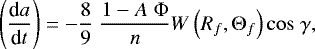
where A is the bond albedo defined by Bowell et al. (1988) and Φ = πR2F(a)∕(mc), where R is the radius of the asteroid, F(a) is the solar flux at the semi-major axis a equal to  (F1au = 1360 W m−2, r is the heliocentric distance of the object), m is the mass of the asteroid, c is the speed of light, γ is the obliquity of the asteroid, and f is the rotation frequency of the asteroid.
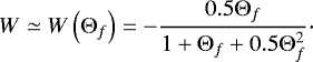
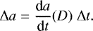
The thermal parameter W from is defined as
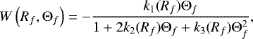 (2)
(2)
where Rf is equal to R∕lf, 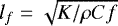 and K is the surface conductivity of the asteroid,C is the surface heat capacity of the asteroid, and ρ is the surface density. Moreover,
 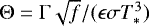 , ϵ is the surface thermal emissivity, σ is the Stefan-Botlzmann constant, and T* is the instantaneous subsolar temperature in thermal equilibrium, which is equal to
 ![Mathematical equation: $\sqrt[4]{(1 - A) F(a)/\epsilon \sigma} $](/articles/aa/full_html/2018/03/aa32079-17/aa32079-17-eq7.png) .
.
2.2 Yarkovsky drift modification caused by D dependence of Γ
Equation (2) can be rewritten assuming k1, k2, k3 = 0.5 for asteroidswith D on the km scale and larger as seen in Fig. 2 of Peterson (1976); Vokrouhlický (1998, 1999)
 (3)
(3)
Approximating Eqs. (1) and (3) for asteroids with identical A, F(a), n, γ, a, r, f, ϵ, and Θf ≫ 1,
 (4)
(4)
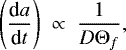
where Θf ∝ Γ. While 1 ≲ Θf ≲ 2, for near-Earth asteroids (Greenberg et al. 2017), Θf ≫ 1 holds true in general for main belt asteroids with D < 40 km, which have an average thermal inertia >100 J m−2 s−0.5 K−1 (Delbo et al. 2015), and where rotation frequencies of km-scale asteroids are typically f ≃ 1 × 10⁻⁴ (Pravec et al. 2002). Combining Θf ∝ Γ with Eq. (4),
 (5)
(5)
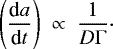
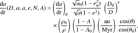
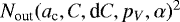
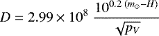
Recent Γ measurements for MBAs and NEOs with D < 100 km suggests that D is related to Γ by the relationship Γ = a Db, where a ≃ 265 J m-2 s-0.5 K-1 and b ≃−0.50 ± 0.08 (Delbo et al. 2015) as seen in Fig. 1. The slope of the correlation b increases to ~ −0.2 ± 0.13 for MBAs and NEOs in the range 0.5 km < D < 100 km, which is the D range of currently observable asteroids in the main belt (Jedicke et al. 2015) as seen in Fig. 2.
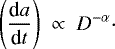
Approximating Eq. (5) with Γ = Db and α = b + 1 we obtain
 (6)
(6)
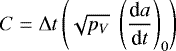
This gives a curvature to the V -shape of the family in a vs. Dr space if α ≠ 1.0. Therefore, following the formulation of the Yarkovsky drift rate from Spoto et al. (2015) combined with Eq. (6), we compute  via the formula
 (7)
(7)
where 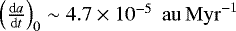 for an asteroid in the inner main belt with a0 = 2.37 au, e0 = 0.2, D0 = 5 km, ρ0 = 2.5 g cm-3, A0 = 0.1, surface conductivity equal to 0.01 W m-1, and obliquity θ0 = 0° (Bottke et al. 2006; Vokrouhlický et al. 2015). Using the values for
  , a0, e0, D0, ρ0, A0, surface conductivity, and θ0 from Bottke et al. (2006) and Vokrouhlický et al. (2015) is appropriate because the value of α is not affected by the values of these variables. For asteroids with 0.5 km < D < 100 km, the value of α that characterizes the curvature of the V -shape of the family should be ~0.8 because b ~−0.2 as indicated bythe D vs. Γ data plottedin Fig. 2. Equation (7) is more appropriate for asteroids of smaller sizes for smaller asteroid families because asteroids of larger sizes that drifted at maximum speed over the entire family age are probably rare and difficult to identify relative to the background. The information in the family V -shape in smaller families is mostly contributed by smaller asteroids because asteroids of larger sizes that drifted at a maximum drift rate described by Eq. (7) over the entire family age are probably rare and difficult to identify relative to the background. Larger families containing asteroids up to a larger size have most of the information in the V -shape in the larger members because the increase in the number of larger asteroids results in the leading edge of the family V -shape becoming adequately populated by asteroids that traveled at the maximum drift rate than when compared to V -shapes of smaller asteroid families.
 |
Fig. 1 D vs. Γ for near-Earth and main belt asteroids of S, C, B, X, and E types and dynamical classes with D < 100 km. The data arefit to the function y = a xb shown as the dark line using orthogonal distance regression (Boggs & Rogers 1990). Measurements of D and Γ are taken from Delbó et al. (2003), Lamy et al. (2008), Delbo & Tanga (2009), Masiero et al. (2011), Müller et al. (2011), Wolters et al. (2011), Marchis et al. (2012), Müller et al. (2012), Müller et al. (2013), Emery et al. (2014), Alí-Lagoa et al. (2014), Müller et al. (2014b), Rozitis & Green (2014), Hanuš et al. (2015), Naidu et al. (2015), Hanuš et al. (2016). |
 |
Fig. 2 Same as Fig. 1, but for near-Earth and main belt asteroids of S, C, B, X, and E types and dynamical classes with 0.5 km < D < 100 km. Measurements of D and Γ are taken from Delbó et al. (2003), Lamy et al. (2008), Delbo & Tanga (2009), Masiero et al. (2011), Müller et al. (2011), Wolters et al. (2011), Marchis et al. (2012), Rozitis & Green (2014), Hanuš et al. (2015,2016), Naidu et al. (2015). |
2.3 Yarkovsky V-shapes
As described in Bolin et al. (2017a), asteroid families whose members’ proper elements e and i have become too dispersed due to chaotic diffusion can be identified by searching for correlations in a vs.  , H space. The size-dependent Yarkovsky force gives a family the V -shape in a vs.
  , H distribution on Myr timescales. In practice, it is possible for a family to obtain a V -shape on shorter timescales due to the contribution of the initial velocity field (Bolin et al. 2017b).
In the standard case of Nesvorný et al. (2003) and Vokrouhlický et al. (2006b) the sides of the V -shape in a vs.  space is
 (8)
(8)
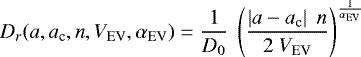
Here Δa is defined as a − ac, where ac is the family center,  is the size-dependent maximal Yarkovsky semi-major axis drift rate, and Δt is the age of the family. The drift rate can be recalculated for different bulk and surface densities, orbit, rotation period, obliquity, and thermalproperties (Bottke et al. 2006; Chesley et al. 2014; Spoto et al. 2015). We define the drift rate
  as formulated in Eq. (7).
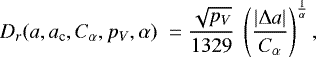
The width of the V -shape in a vs.  space can be defined by the constant C assuming the case, where α = 1.0 is
 (9)
(9)
from Vokrouhlický et al. (2006b) where pV is the geometric albedo, which is assumed to be the average albedo for family members (an assumption well supported by observations; Masiero et al. 2013), and  is the same as in Eq. (7). Typical pV values of 0.05 and 0.15 are used for C- and S-type asteroids, respectively (Masiero et al. 2011, 2015).
Combining Eqs. (8), (7), and (9), we define the border of the V -shape in reciprocal diameter,  or Dr, space as
 (10)
(10)
where Cα in Eq. (10) is normalized to a value of C with the factor
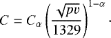 (11)
(11)
Equation (10) is rewritten in terms of (a, ac, C, pV, α) by using Eq. (11):
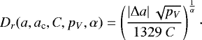 (12)
(12)
Two generic V -shapes are plotted in Fig. 3 using Eq. (12) and 1.0 and ~0.8 for the value of α and shows how the curved V -shape line crosses the straight V -shape border at Dr = 1.0.
 |
Fig. 3 Two generic family V -shapes with ac= 2.37 au and C = 1.9 × 10⁻⁵ au and α = 0.8, 1.0. |
2.4 V-shape identification technique and measurement of α
Family V-shape’s ac, C, and α are measured according to Eq. (12) in a vs. Dr space with the V -shape border method described in Bolin et al. (2017a,b): the location of the border of the V -shape described by ac, C, and α in Eq. (12) are determined by maximizing the ratio of the number of objects inside a V -shape border, Nin, to the number of objects located outside the border, Nout, where Nin and Nout are described by the following equations:
 (13)
(13)
 (14)
(14)
Equations (14) and (13) are normalized the area in a vs. Dr between the nominal andouter V -shapes defined by Dr(a, ac, C+, pV, α) and Dr(a, ac, C, pV, α) in the denominator of Eq. (14) and between the nominal and inner V -shapes defined by Dr(a, ac, C, pV, α) and Dr(a, ac, C−, pV, α) in the denominator of Eq. (13).
The symbol Σj in Eqs. (14) and (13) indicates summation on the asteroids of the catalog, with semi-major axis aj and reciprocal diameter Dr,j. The symbol δ indicates Dirac’s function, and a1 and a2 are the low and high semi-major axis range in which the asteroid catalog is considered. The function w(D) weighs the right-side portions of Eqs. (14) and (13) by their size so that the location of the V -shape in a vs. Dr space will be weighted towards its larger members. The exponent 2.5 is used for w(D) = D2.5, in agreement with the cumulative size distribution of collisionally relaxed populations and with the observed distribution for MBAs in the H range 12 < H < 16 (Jedicke et al. 2002).
Walsh et al. (2013) found that the borders of the V -shapes of the Eulalia and new Polana family could be identified by the peak in the ratio  where Nin and Nout are the number of asteroids falling between the curves defined by Eq. (12) for values C and C− and C and C+, respectively, with C− = C −dC and C+ = C + dC. We extend our technique to search for a peak in the ratio
  , which corresponds to weighting the ratio of
  by the value of Nin. This approach has been shown to provide sharper results (Delbo’ et al. 2017). We consider only asteroids in the border of the V -shape because the functional form of the V -shape may become distorted inside the V -shape border due to varying obliquity reorientation rates with asteroid size (Paolicchi & Knežević 2016).
Whereas Walsh et al. (2013) and Delbo’ et al. (2017) assumed α = 1.0 and searched for a maximum of  in the space ac, C, here we perform the maximum search in three dimensions in the space ac, C, and α. The three-dimensional search is tested on a synthetic family generated as described in Sect. 3.1 producing a peak value in
 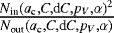 indicated by the black rectangle in the top panel of Fig. 4. For simplicity, in the top panel of the figure we plot the value of the ratio on the α, C plane for the value of ac that maximizes the ratio in each cell. The V -shape that maximizes the ratio is plotted in the bottom panel, together with the asteroids of the family using Eq. (12) as seen in the bottom panel of Fig. 4.
The value of dC is used as it is in Bolin et al. (2017a) and Bolin et al. (2017b). The value of d C used depends on the density of asteroids on the family V -shape edge. The value of dC can be 10%–30% of the V -shape’s C value if the density of asteroids on the V -shape edge is high, as in the case of the Massalia family discussed in Sect. A.1.2 and more, up to 40–50% if the V -shape edge is more diffuse, as inthe case of the Dora(2) subfamily discussed in Sect. A.2.4 (Nesvorný et al. 2015). The inner and outer V -shapes must be wide enough to include enough asteroids in the inner V -shape and measurea ratio of  to Nout that is high enough to identify the family V -shape. Only asteroids that belong to the nominal the hierarchical clustering method (HCM) classification of the family are used instead of the full catalog of asteroids. The nominal family classification can include interlopers that the V -shape technique can include if the value of dC used is too large (Nesvorný et al. 2015; Radović et al. 2017). Asteroids that fall out of the best fit V -shape with a reasonable value of dC may be trueinterlopers even if nominal members of the HCM defined family.
The V -shape identification technique was tested on families identified by both Nesvorný et al. (2015) and Milani et al. (2014), such as the Erigone family to verify that the V -shape ac, C, and α determination on family membership definitions from either database produces the same results as seen in Figs. 5 and 6 and discussed for the Erigone, Massalia, Agnia, and Maria family in Sects. A.1.1, A.1.2, A.2.1, and A.3.4, respectively.
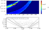 |
Fig. 4 Application of the V -shape identification to synthetic asteroid family data at Time = 200 Myr. Top panel: the ratio of
|


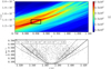 |
Fig. 5 Same as Fig. 4, but for the Erigone asteroid family data from Nesvorný et al. (2015). Top panel: Δα is equal to 1.8 × 10⁻³ au, and ΔC is equal to 9.0 × 10⁻⁸ au. Bottom panel: Dr(a, ac, C ± dC, pV, α) is plotted with pV = 0.05, ac = 2.796 au, and dC = 7.5 × 10⁻⁶ au. |
2.5 Data set and uncertainties of α measurements
2.5.1 Data set
The data used to measure the V -shapes of asteroid families were taken from the Asteroid Dynamic Site1 (AstDys) forthe H magnitudes. The offset between H magnitudes from the MPC and individually calibrated magnitudes from Pravec et al. (2012) and Vereš et al. (2015) is assumed to be constant for objects in the range 12 < H < 18 (Vereš et al. 2015). Family definitions were taken from Nesvorný et al. (2015). Asteroid family data for the Erigone, Massalia, Agnia, Eunomia, Hoffmeister, Maria, and Ursula families were used from both Milani et al. (2014) and Nesvorný et al. (2015). Family visual albedo, pV, data from Masiero et al. (2013) and Spoto et al. (2015) were used to calibrate the conversion from H magnitudes to asteroid D using the relation 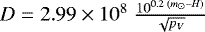 (Bowell et al. 1988), where m⊙ = −26.76 (Pravec & Harris 2007). Numerically and analytically calculated MBA proper elements were taken from AstDys (Knežević & Milani 2003). Numerically calculated proper elements were used preferentially and analytical proper elements were used for asteroids that had numerically calculated elements as of September 2017.
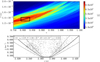 |
Fig. 6 Same as Fig. 5, but repeated for the Erigone family defined by Milani et al. (2014). |
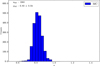 |
Fig. 7 Histogram of α
located at the peak value of |
2.5.2 Uncertainty of α
The value of α located where  peaks in α vs. C space represents the best estimate of the α of an asteroid family’s V -shape using the nominal a and Dr asteroid values. Differences between family members in their physical properties cause a spread in possible α values; when measured together they increase the uncertainty on the measured value of α. Variation between family members’ D is directly caused by the uncertainty on their H magnitudes and pV measurements. In addition to the uncertainty on the asteroids’ D, lack of complete information about the true population of asteroids within a family and the outliers contribution to a family’s a vs. Dr distribution can increase the range of uncertainty on α values compatible with the family V -shape. We devised the following Monte Carlo procedure to quantify the variation in α taking into account these affects.
At least 1200 Monte Carlo trials are completed per family. In each trial, the location of the peak  value in α vs. C is recorded. Three steps are completed to randomize the asteroid family data from the original a vs. Dr distribution per trial. The first step is to create a resampled data set of family fragments by removing
  objects randomly where N is the number of objects ina vs. Dr space in order to include variations caused by incomplete knowledge of the asteroid family’s population. Incompleteness of asteroid family fragments increases for smaller fragments and is more pronounced in the central and outer portions of the main belt (Jedicke & Metcalfe 1998; Jedicke et al. 2002), and the increased incompleteness and greater number of smaller main belt asteroids in the asteroid family catalogs causes the variation in α to be weighted towards smaller fragments than larger fragments.
A second step is taken to determine the variation caused by incomplete information in the family fragment population by resampling the fragments’ a by their own a distribution. In this step, a continuous distribution interpolating the a values of family fragments per Dr bin is generated and used to reassign the fragments’ new a values. The bin size of Dr used is 0.001 km−1 for all asteroid families.
The third step is to randomize the measurements of H and pV of the asteroids by their known uncertainties. Asteroid H values were varied per Monte Carlo run by adding a random value between –0.25 and 0.25 mag equal to the known uncertainties for H values from the MPC catalog (Oszkiewicz et al. 2011; Pravec et al. 2012). Asteroid fragments’ H values are converted toD after their H values are randomized using the following equation
 (15)
(15)
from Harris & Lagerros (2002), and a value of pV chosen at random for each asteroid using central values and uncertainties per asteroid family from Masiero et al. (2013) and Spoto et al. (2015).
The mean and root mean square (RMS) uncertainty on α was determined from the distribution of the values of α determined in each of the Monte Carlo trials. Having more fragments and a well-defined V -shape causes the Monte Carlo technique to produce a narrower distribution in α (e.g., for the Erigone family, α = 0.83 ± 0.04, Fig. 7), while having fewer fragments and a more diffuse V -shape results in a broader α distribution (e.g., for the Misa subfamily, α = 0.87 ± 0.11, Fig. 8).
2.6 Family ages
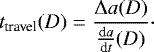
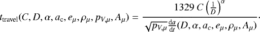
The time of travel for an individual asteroid with diameter D is
 (16)
(16)
The asteroidtravel time as a function of C; asteroid diameter D, α, the V -shape center ac, average eccentricity of asteroid family members eμ, the average family member density ρμ, the average family member visual albedo pV,μ, and the average family member bond albedo Aμ is found by combining Eqs. (12) and (16) and expanding the denominator of Eq. (16) to include  as a function of D, α, ac, eμ, ρμ, and Aμ:
 (17)
(17)
Equation (17) assumes no initial dispersion in the asteroid family due to the initial ejection velocity field. In reality this initial dispersion exists. The value of C measured from the distribution of asteroid family members in reality includes the contribution of the initial ejection velocity field from Eq. (19) and the contribution to C from the Yarkovsky effect (Vokrouhlický et al. 2006b; Nesvorný et al. 2015),
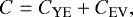 (18)
(18)
where CYE is the width of the V -shape due to the Yarkovsky effect described byEq. (9) and CEV is the width of the V -shape due to the initial ejection velocity of fragments described by (Vokrouhlický et al. 2006b; Bolin et al. 2017b)
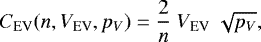 (19)
(19)
where n is the mean motion of the parent body and V EV is a parameter describing the width of the fragment velocity distribution (Michel et al. 2004; Nesvorný et al. 2006; Durda et al. 2007; Vokrouhlický et al. 2017b). The nominal value of CEV can exceed more than 50% of C for asteroid families younger than 100 Myr (Nesvorný et al. 2015; Carruba & Nesvorný 2016). The error on the estimate of the initial ejection velocity field can be large enough so that there is a possibility that C − CEV ≲ 0 for young asteroid families, but we assume asteroid families considered in this study are all at least ≳20 Myr old and will have C − CEV > 0.
The contribution of the initial ejection of the fragments must be subtracted from the calculation of ttravel (Nesvorný et al. 2002; Carruba & Nesvorný 2016; Carruba et al. 2016b). The value of C includes the contribution from the spread in a of the fragments caused by their initial ejection velocities in addition to their spread caused by the Yarkovsky effect:
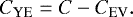 (20)
(20)
The age of the family is found by using CYE and expanding  from Eq. (7) in the denominator of Eq. (17) and then simplifying
 (21)
(21)
We simplify A in Eq. (21) according to A = pV (0.290 + 0.684 G) from Harris & Lagerros (2002) to only include pV and G in the formulation
 (22)
(22)
where pV,0 = 0.2 and G0 = 0.24.
The ages determined by Eq. (22) are valid for families <2 Gyr old because the Sun’s luminosity has varied by ≲10% over the last 2 Gyr (Bertotti et al. 2003). Equation (22) is modified to include changing luminosity of the Sun for families older than 2 Gyr (Vokrouhlický et al. 2006b; Carruba et al. 2016c)
![Mathematical equation: \begin{multline*}t_{\textrm{age}>2~\textrm{Gyr}}(C_{\textrm{YE}},\alpha,a_{\textrm{c}},e_{\mu},\rho_{\mu},p_{V,\mu},G_{\mu}, t_1) = \\\frac{t_{\textrm{age}}(C_{\textrm{YE}}, \alpha,a_{\textrm{c}},e_{\mu},\rho_{\mu},p_{V,\mu},G_{\mu}) }{ \left (\frac{1}{4.57 \; \mathrm{Gyr} - t_1}\int\limits_{t_1}^{4.57 \; \mathrm{Gyr}}\left[1.3 + \frac{0.3 t}{4.57 \; \mathrm{Gyr}} \right ]^{-1} \textrm{d}t \right )} ,\end{multline*}](/articles/aa/full_html/2018/03/aa32079-17/aa32079-17-eq51.png) (23)
(23)
where t1 is the epoch of the family’s formation in Gyr measured from the beginning of the solar system. Equation (23) does not include the evolution of the fragments’ pV caused by space weathering on secular timescales (e.g., Jedicke et al. 2004; Vernazza et al. 2009).
Family ages calculated with Eqs. (22) and (23) using the values of ac, C, and α determined by the V -shape determination technique described in Sect. 2.4 can differ from the previous family ages obtained assuming α = 1.0 (Vokrouhlický et al. 2006b; Brož et al. 2013; Spoto et al. 2015). Unlike in the case where family ages that are recomputed with the stochastic Yarkovský O’Keefe Radzievskii Paddack (YORP) effect model are always younger than their previously determined ages (Bottke et al. 2015; Carruba et al. 2016c), family ages calculated with variable α, t(CYE,α, α), or tage >2 Gyr(CYE,α, α), can be younger, the same, or older than t(Cy,α=1) or tage>2 Gyr(Cy,α=1) when  ,
,  , or
, or  , respectively.
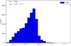 |
Fig. 8 Same as Fig. 7, but for ~4400 trials repeating the V -shape technique for the Misa family. The mean of the distribution is centered at α = 0.87± 0.11 and the bin size in the histogram is 0.04. |
3 Results
3.1 Synthetic family
The V -shape ac, C, and α determination technique is tested on a synthetic asteroid family where fragments are initially dispersed simulating the disruption of a parent bodyand then are allowed to evolve for several hundred Myr under planetary perturbations and the Yarkovsky effect. The V -shape determination technique is applied to the synthetic asteroid family’s V -shape to measure its ac, C, and α and ensure they match the values assumed for the generation of the synthetic family in the simulation.
The breakup of a synthetic asteroid family and the subsequent evolution of its fragments due to the Yarkovsky effect is simulated by using 650 particles at  and distributed in a vs. Dr space according to
 (24)
(24)
from Vokrouhlický et al. (2006b); Bolin et al. (2017b), where αEV is the exponent scaling V EV with D (Cellino et al. 1999). A value of αEV = 1.0 was used based on recent work on ejection velocity V -shapes of young asteroid families indicating that αEV ≃ 1 (Bolin et al. 2017b). D0 = 5 km and V EV = 30 m s-1 using fragments with 2 km < D < 75 km distributed according to the known members of the Erigone family defined by Nesvorný et al. (2015). The eccentricity and inclination distributions of the ejected fragments were determined by using Gaussian scaling described in Zappalà et al. (2002). The value of the ejection velocity, V EV = 30 m s-1 corresponds to a typical initial displacement of ~ 7.0 × 10⁻³, where given V EV, the displacement in a is size-independent.
The Yarkovsky drift rates were defined via Eq. (7) with  , a0 = 2.37 au, e0 = 0.2, D0 = 5 km, ρ0 = 2.5 g cm-3; the Bond albedo A0 is equal to 0.1, the surface conductivity equal to 0.01 W m-1 K-1, and θ0 = 0° (Bottke et al. 2006; Vokrouhlický et al. 2015). For the synthetic family, ρ = 2.3 g cm-3, A = 0.02, and cos (θ) is uniformly distributed between –1 and 1. The Yarkovsky drift rate was scaled with D−α≃−0.8 (now defined as αYE for the Yarkovsky effect) as suggested bythe relationship between D and Γ data for current asteroid data with 0.5 km < D < 100 km discussed in Sect. 2.2. The particles were evolved with the Yarkovsky effect and gravitational perturbations from Mercury, Venus, Earth, Mars, Jupiter, and Saturn using the SWIFT_RMV S code (Levison & Duncan 1994). Particles are removed from the simulation if they collide with one of the planets or evolve into orbits that have a perihelion of 0.1 au. YORP rotational and spin-axis variation are not included in the simulation.
The V -shape identification technique was applied on the synthetic family data at Time = 200 Myr using the techniques in Sect. 2.4. As discussed in Bolin et al. (2017b), the time it takes for the V -shape of the synthetic Erigone family to transitionfrom having its α = αEV equal to 1.0 to α equal to αYE ≃ 0.8 is ~20 Myr. Measuring aV -shape’s α using synthetic family data from time steps after 20 Myr will be measuring the V -shape’s αYE. Equations (14) and (13) are integrated using the interval (− ∞,∞) for the Diracdelta function δ(aj − a) and the interval [0.04, 0.60] for the Dirac delta function δ(Dr,j − Dr). Equation (12) is truncated to 0.04 km−1 for Dr < 0.04 km−1 and to 0.60 km−1 for Dr > 0.60 km−1. Asteroids with 0.04 < Dr < 0.60 were chosen because the number of asteroids in this Dr is large enough so that the leading edge of the V -shape is defined by asteroids with cos(θ) = 1.0 or –1.0 according to Eq. (12).
The V -shape identification technique located a peak at (ac, C, α) = (2.367 au, 2.8 × 10⁻⁵ au, 0.8) as seen in the top panel of Fig. 4. The peak value of  is ~8 standard deviations above the mean value of
  in the range 2.25 au < a < 2.45 au, 1.0 × 10⁻⁵ au < C < 3.5 × 10⁻⁵ au, and 0.6 < α < 1.4. A d C = 8.0 × 10⁻⁶ au were used. The concentration of the peak to one localized area in α vs. C space is due to the sharpness of the synthetic family’s V -shape border. The procedure was repeated again using only larger asteroids in the synthetic family with 5 km < D < 10 km to determine whether this resulted in a different values of α than when using V -shapes consisting of a full range of smaller asteroids. We did not measure any significant difference between the values of α measured inthe two cases.
3.2 Mainbelt asteroid families
The V -shape ac, C, and α determination technique was applied to 26 asteroid families located through the inner, central, and outer main belt. Proximity to mean motion and secular resonances can remove asteroids from an asteroid family resulting in an incomplete V -shape. Asteroid families were divided into three categories: complete V -shapes, clipped V-shapes (where one or both sides ofa family V -shape do not form a full V), and half V -shapes (where only one side of the V -shape is complete). Completeness of the V -shape does not change the functional form of the V -shape technique described in Sect. 2.4, but affects the range of asteroids used in the technique, as will be described in the following sections. All families are assumed to be old enough so that C −CEV > 0 and therefore their measured value of α = αYE as discussed in Sect. 2.6.
3.2.1 Complete V-shape families
An asteroid family with a complete V -shape is defined as having a complete V -shape in extent along the a axis relative to the center of the V -shape in a vs. Dr space such as the Erigone family seen in the bottom panel of Fig. 5. Equations (14) and (13) are integrated using the interval (− ∞, ∞) for the Dirac delta function δ(aj − a) due to their symmetric shape. It has been noted that the V -shapes of some families such as the Erigone family are non-symmetric in the value of C between the inward and outward halves of their V -shapes (Spoto et al. 2015). We do not find significant differences in C between the inner and outer V -shape halves of asteroid families and therefore fit the families with a unique value of C. The interval for the Dirac delta function δ(Dr,j − Dr) is chosen with respect to the range in Dr that contains the complete V -shape of the family.
The measured values of α and their uncertainties, family ages, and the physical properties assumed for each family in the measurement for four complete V -shape families using the techniques described in Sects. 2.4, 2.5.2, and 2.6 for each of the complete V -shape families are summarized in Table 1. A description of how the V -shape determination technique is implemented for each complete V -shape family is described in Sect. A.1.
3.2.2 Clipped V-shape families
An asteroid family with a clipped V -shape is defined as having at least one full V -shape half in addition to another partial V -shape, such as the Agnia family seen in the bottom panel of Fig. 9 where the outer V -shape half is depleted of asteroids at about Dr = 0.4 km−1 because it is intersected by the 5:2 MMR with Jupiter at 2.82 au. Intervals used for integrating Eqs. (14) and (13) for the Dirac delta function δ(aj − a) are (−∞, ac] when applying the V -shape technique to only the complete inner V -shape half, [ac, ∞) when applying the technique to only the complete outer V -shape half, and (−∞, ∞) when applying the technique to both the complete and incomplete halves. The interval used for δ(aj− a) is determined by whether or not there are enough asteroids in the complete V -shape borders to obtain a statistically robust determination of α.
As discussed in Sect. 3.2.1, we assume that the values of C and α are the same on both V -shape halves. The measured values of α and their uncertainties, family ages, and the physical properties assumed for each family are summarized in Table 2. A description of how the V -shape determination technique is implemented for 12 clipped V -shape families is described in Sect. A.2.
Complete V -shape families.
 |
Fig. 9 Same as Fig. 4, but for Agnia asteroid family data from Nesvorný et al. (2015). Top panel: Δα is equal to 1.4 × 10⁻² au, and ΔC is equal to 7.4 × 10⁻⁷ au. Bottom panel: Dr(a, ac, C ± dC, pV, α) is plotted with pV = 0.18, ac = 2.791 au, and dC = 7.5 × 10⁻⁶ au. |
3.2.3 Half V-shape families
An asteroid family with a half V -shape is comprisedof only one full V -shape in a vs. Dr space, such as the Eulalia family seen in the bottom panel of Fig. 10 where the family’s V -shape center is located within the vicinity of the 3:1 MMR with Jupiter at 2.5 au. The Dirac delta function δ(aj− a) in Eqs. (14) and (13) is integrated using the interval (− ∞,ac] or [ac, ∞) for the half V -shape case.The interval for the Dirac delta function δ(Dr,j − Dr) is chosen to include the full Dr range encompassing the half V -shape in a vs. Dr space.
The measured values of α and their uncertainties, family ages, and the physical properties assumed for each family are summarized in Table 3. A description of how the V -shape determination technique is implemented for ten clipped V -shape families is described in Sect. A.3.
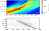 |
Fig. 10 Same as Fig. 4, but for the Eulalia asteroid family data from Nesvorný et al. (2015). Top panel: Δα is equal to 7.5 × 10⁻³ au, and ΔC is equal to 8.0 × 10⁻⁷ au. Bottom panel: Dr(a, ac, C ± dC, pV, α) is plotted with pV = 0.05, ac = 2.49 au, and dC = 3.2 × 10⁻⁶ au. |
4 Discussion and conclusion
The dependence of thermal inertial of asteroids on asteroids’ physical sizes suggests that the size dependence of the Yarkovsky semi-major axis drift should be proportional to Dα with α < 1. We have analyzed the V -shape in the a vs. Dr distribution of 26 families and determined the value of α that best characterizes these shapes. We have analyzed the V -shapes of families located in the inner, central, and outer main belt and determined their ages. Although the 26 families used in this study represent only a quarter of the ~110 known asteroid families defined by Nesvorný et al. (2015), they constitute a representative sample of asteroid families in the main belt because the families in the sample are spread evenly through the inner, central, and outer main belt and cover the main taxonomic types of asteroids
The statistical uncertainty (standard deviation) on the determination of α was estimated using a Monte Carlo technique, as described in Sect. 2.5.2. We found that the difference between the measured value of α and α = 1.0 is more than three times the standard deviations for the majority of family V -shapes. This suggests that the curvature of family V -shapes in a vs. Dr space is realand widespread throughout the families in the main belt. In a different study (Bolin et al. 2017b), which focuses on young families dominated by the initial ejection velocity field, we determined that α = 1.0. Thus, the values of α different from 1 that we obtain in this paper should be attributed to the non-trivial size dependence of the Yarkovsky drift speed. The average value of α of the 26 family Yarkovsky V -shapes in this study is 0.87 ± 0.01, or within the Student’s t-distribution 99.8% confidence interval of 0.86–0.87. The average value of α when considering only the 8 S-type families and the 16 C-type families with α measurements separately are statistically indistinguishable.
The measured values of α changes throughout the main belt with the α of the asteroid family V -shapes in the inner and central main belt (defined as 1.8 au < a < 2.5 au and 2.5 au < a < 2.8 au, respectively) having a lower α value on average, αμ ≃ 0.84 ± 0.01, than that of families in the outer belt (defined as 2.8 au < a < 3.3 au, αμ ≃ 0.91 ± 0.01) as seen in Fig. 11. A linear fit to the results in ac vs. α space is significantly sloped with α = a x + b, where a = 0.1 ± 0.03 au−1, x = ac, and b = 0.57 ± 0.09, as seen in Fig. 11. There is some indication that this slope is somewhat steeper if we restrict ourselves to the 8 S-type family V -shapes spread throughout the inner, central, and outer main belt. In this case we find α ≃0.2 au−1 ± 0.07 overlapping with the slope including families of all taxonomic types. Instead, there is no change in slope when considering only the 16 C-type families.
The inward curvature of V -shapes in a vs. Dr space with α < 1.0 suggests that objects smaller than ~1 km are drifting slower and larger objects are drifting faster compared to the case with α = 1.0. A possible explanation for the inward curvature of family V -shapes and the slower drift rate of small asteroids is the dependence of thermal inertia on D, first described by Delbo et al. (2007). The average α = 0.87 ± 0.01 of family V -shapes overlaps with the value of α = 0.77 ± 0.13 expected from the relationship in D vs. Γ space for asteroids with 0.5 km < D < 100 km as described in Sect. 2.2. Additionally, the planetary regolith model of Gundlach & Blum (2013), which determines surface regolith size from an asteroid’s Γ, surface temperature, and taxonomic type predicts a slight increase in the linear slope of D vs. Γ for the outer main belt families, which corresponds to a ~ 10% higher α for asteroid families in the outer main belt compared to asteroid families in the inner main belt. This is in good agreement with the difference in the mean value of α between inner and outer main belt family V -shapes determined in this paper, although this difference is also comparable to the relative uncertainty of the model of Gundlach & Blum (2013).
Some caution must be used when comparing α measurements determined from asteroid family V -shapes with the α expected from the asteroid’s D vs. Γ relationship because the spin rate of an asteroid can affect its Γ. In fact, slower spinning asteroids, i.e., those with rotation periods greater than 10 h, may have a higher Γ than more quickly spinning asteroids possibly as a result of rapidly increasing material density and Γ with surface depth (Harris & Drube 2016). Additionally, thermal inertia is expected to have a heliocentric dependence as a result of its temperature dependence.
One explanation for the apparent increase of α towards 1.0 with heliocentric distance is that asteroid family members in the outer belt have similar regolith properties. An increase in α to 1.0 for an asteroid family V -shape implies that there is no decrease in Γ with increasing D as observed in the general asteroid population if α is assumed to be an indication of the linear slope in D vs. Γ space for individual asteroid family members. As discussed in Sect. 1, small and large asteroids have different surface regolith properties with small asteroids having coarser regolith resulting in larger values of Γ compared to larger asteroids. A more even distribution in Γ between larger and smaller asteroids would imply that small and large asteroids have either coarse or fine regolith.
One possible source of surface regolith coarseness homogenization between small and large asteroids is that recent family creation produces vast quantities of dust coating the surfaces of the members of other asteroid families in the vicinity. The outer belt contains a higher proportion of young asteroid families that were created within the last 20 Myr, such as the 1993 FY12, Brasilia, Iannini, Karin, König, Koronis(2), Theobalda and Veritas asteroid families (Nesvorný et al. 2015; Bolin et al. 2017b), some of which have been attributed as the source of the IRAS dust bands (Grogan et al. 2001; Nesvorný et al. 2003). Enough dust would have to be produced and accreted onto a significant number of asteroids within a family and homogenize the surface regolith properties between members to have a significant effect in changing the curvature of the family V -shape.
The ages of asteroid families are calculated with Eqs. (22) and (23) with α determined by the V -shape technique and plotted in Fig. 12. The family V -shape α are normalized to 1 au with respect to ac according to α = 0.11 ± 0.03 ac + 0.57 ± 0.09 determined from the linear fit in Fig. 11. The αnormalized of family V -shapes describes the relative amount of curvature of a family V -shape if all family V -shapes had the same ac. Higher values of αnormalized correspond to V -shapes with less curvature compared to lower values of αnormalized. The resulting fit in Revised Age vs. αnormalized space is compatible with no trend in increasing or decreasing curvature with age. The slope is only 0.03 with a relatively large uncertainty of 0.01 due to large uncertainties in the linear slope of asteroid V -shape data in ac vs. α space and the large uncertainties on the age of asteroid families as discussed in Sect. 2.6.
The curvature of the V -shape of asteroid families is similar to that produced by the “stochastic YORP” effect (Bottke et al. 2015). The stochastic YORP model applied to asteroid family V -shapes describes the YORP states of individual family fragments where they are reset or modified by minute changes in their shapes or surface features (Statler 2009; Cotto-Figueroa et al. 2015). When applied to asteroid families, the stochastic YORP model entails that the functional form of asteroid family V -shape described by Eq. (12) with α = 1.0 becomes distorted or inwardly curved as asteroid families age, particularly for asteroid families older than 500 Myr and for asteroids smaller than ~1 km. This effect of stochastic YORP is similar to the effect of size-dependent Γ on asteroid family V -shapes described by Eq. (12) with α < 1.0.
However, the lack of a clear trend with decreasing αnormalized with increasing age, i.e., asteroid families becoming more curved with age, suggests that smaller, D 1 ~ 3 km asteroids may not be as affected by stochastic YORP cycles as predicted by (Bottke et al. 2015) for asteroid families 500 Myr to ≳2 Gyr old. In fact, the oppositetrend seems to be the case because some Gyr-old families such as the Eos, Hygiea, Koronis, Ursula, and Nemausa have less curvature, (i.e., α ~ 0.9) compared to families with ages <500 Myr such as the Astrid, Erigone, Massalia, Naema, and Tamara (0.7 ≲ α ≲ 0.8) suggesting that the overall trend between family ages and α seems to be inconclusive or unfavorable to the stochastic YORP model when applied to asteroid family V -shapes. More importantly, the lower bound in asteroid size used in the V -shape determination technique excludes asteroids affected by the stochastic YORP. For instance, in the case of the Eunomia, Hygiea, and Koronis families the smallest asteroids used were ~7 km, much larger than the 1–2 km size at which the stochastic YORP becomes apparent. However, one possibility is that the timescale on which YORP becomes stochastic for asteroids is longer than predicted by Bottke et al. (2015), as indicated by recent simulations of the evolving shapes of certain asteroids due to rotational stress resulting in less change on asteroid family V -shapes (McMahon 2017). Instead of stochastic YORP having an effect on an asteroid family’s V -shape after 500 Myr, it may take an effect on much longer timescales than can be recognized within the range of ages of asteroid families studied in this paper.
An alternative explanation of curved family V -shapes is that family fragments are non-uniform in density, with smaller fragments having a higher density compared to larger objects, resulting in lower drift rates for smaller asteroid as determined by Eq. (7). Additionally, reaccumulation of material following the disruption of the parent body with uniform density may result in less dense larger fragments (Michel et al. 2001, 2015). In fact, larger fragments have greater gravity and are able to reaccumulate more debris into a more loosely compact body than smaller fragments.
However, bulk density measurements of S- and C-type 50–200 km asteroids are relatively homogenous with a slight increase in ρ for larger objects past 200 km (Carry 2012). This increase in ρ at larger asteroid sizes is possibly due to grain compaction (Consolmagno et al. 2008), but it is beyond the size affected by the Yarkovsky effect (Vokrouhlický et al. 2015). Measured bulk densities of small km-scale asteroid bodies from spacecraft missions (such as the NEAR-Shoemaker mission to Eros Yeomans et al. 2000, Hayabusa spacecraft’s mission to Itokawa Fujiwara et al. 2006 and the Rosetta spacecraft’s flyby of Lutetia Drummond et al. 2010), the YORP effect (Lowry et al. 2014), or observation of binaries (Hanuš et al. 2017; Carry et al. 2015; Margot et al. 2015) are comparable to their larger counterparts suggesting that there is no size dependence on asteroid ρ for asteroids in the sub-km to 10 km scale.
The weak dependence of ρ with size would cause asteroid family V -shapes to have no curvature or be slightly curved with α ≳ 1.0, which is opposite to the α < 1.0 measured for family V -shapes throughout the main belt. This implies that the inward curvature of asteroid family V -shapes is probably not caused by density inhomogeneities with asteroid size within a family.
Although the main goal of this study is not to redetermine the ages of asteroid families, the ages of asteroid families calculated with Eqs. (22) and (23) with α V -shape measurements can be compared to ages calculated assuming α = 1.0 (e.g., Brož et al. 2013; Spoto et al. 2015). The age of asteroid families revised with α measurements as described in Sect. 2.6 are summarized in Tables 1, 2, and 3. The average relative difference between the revised age and the age determined with α = 1.0 is –12 ± 26% implying that the ages of asteroid families are overestimated on average when α is assumed to be unity. The absolute relative difference between asteroid family ages calculated with V -shape technique determined α and α = 1.0 is on average 22 ± 19%.
Clipped V -shape families.
Half V -shape families.
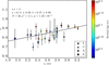 |
Fig. 11 ac vs. α vs. revised age for asteroid families of all taxonomies. The Eos asteroid family is labeled as an S-type in this plot. The data are fit to the function y = a x + b in ac vs. α space, which is shown as the dark line using orthogonal distance regression (Boggs & Rogers 1990). |
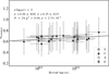 |
Fig. 12 Age vs. α for asteroid families of all taxonomies. The data are fit to the function y = a log10(x) + b shown as the dark line using orthogonal distance regression (Boggs & Rogers 1990). |
Appendix
A.1 Complete V-shape families
A.1.1 Erigone
The Erigone asteroid family located in the inner main belt was first identified by Zappalà et al. (1995) and consists of mostly C-type asteroids (Masiero et al. 2013; Spoto et al. 2015). The V -shape identification technique was applied to 1742 asteroids belonging to the Erigone asteroid family as defined by Nesvorný et al. (2015). Equations (14) and (13) are integrated with the interval [0.04, 0.73] for the Dirac delta function δ(Dr,j − Dr). Equation (12) is truncated to 0.04 km−1 for Dr < 0.04 km−1 and to 0.73 km−1 for Dr > 0.73 km−1. Asteroid H values were converted to D using Eq. (15) using the value of pV = 0.05 typical for members of the Erigone family (Masiero et al. 2013; Spoto et al. 2015).
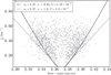 |
Fig. A.1 a
vs. |

The ratio  at (ac, C, α) = (2.37 au, 1.34 × 10⁻⁵ au, ~0.85) is shown in the top panel of Fig. 5 and is ~3 standard deviations above the mean value of
  . The technique was repeated with the joint Erigone and Martes family defined by Milani et al. (2014) resulting in similar results to those seen in Fig. 6. We repeated the process in ~2000 Monte Carlo runs where the physical parameters of the family fragments were randomly varied in each run as described in Sect. 2.5.2. The pV of asteroids in the Monte Carlo trails was assumed to be the average value of pV for family fragments in the Erigone family fragments of 0.05 with an uncertainty of 0.01 (Spoto et al. 2015). The Monte Carlo trial values of α is ~0.83 with a RMS uncertainty of 0.04 as seen in Fig. 7. The Erigone family V -shape is better fit with α = 0.83 than the V -shape with α = 1.0, as seen in Fig. A.1.
The family age of 90 ± 40 Myr is calculated using Eq. (22), with CYE = 5.6 × 10⁻⁶ au calculated from Eq. (20) where C = 1.35 × 10⁻⁵ au. The value ofμα = 0.83 and CEV = 7.90 × 10⁻⁶ au are calculated using Eq. (19) assuming V EV = 30 m s-1 from Vokrouhlický et al. (2006b). We note that the 90 Myr age from this estimate is the same minimum amount of time needed to maintain a steady state population of C-type asteroids in the z2 resonance that interacts with members of the Erigone family (Carruba et al. 2016a).
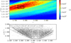 |
Fig. A.2 Same as Fig. 4, but for Massalia asteroid family data from Nesvorný et al. (2015). Top panel: Δα is equal to 1.8 × 10⁻³ au, and ΔC is equal to 5.0 × 10⁻⁷ au. Bottom panel: Dr(a, ac, C ± dC, pV, α) is plotted with pV = 0.24, ac = 2.41 au, and dC = 5.0 × 10⁻⁶ au. |
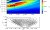 |
Fig. A.3 Same as Fig. A.2, but repeated for the Massalia family defined by Milani et al. (2014). |
A.1.2 Massalia
The Massalia asteroid family located in the inner main belt was first identified by Zappalà et al. (1995) and consists of mostly S-type asteroids (Masiero et al. 2013; Spoto et al. 2015). The V -shape identification technique was applied to 6414 asteroids belonging to the Massalia asteroid family as defined by Nesvorný et al. (2015). The interval [0.09, 2.2] for the Dirac delta function δ(Dr,j − Dr) is used and Eq. (12) is truncated to 0.04 km−1 for Dr < 0.04 km−1 and to 0.73 km−1 for Dr > 0.73 km−1. Asteroid H values were converted to D using Eq. (15) and a value of pV = 0.24 typical for members of the Massalia family (Masiero et al. 2013; Spoto et al. 2015). The peak in  at (ac, C, α) = (2.41 au, 1.95 × 10⁻⁵ au, ~0.76). The technique was repeated with the Massalia family defined by Milani et al. (2014) resulting in similar results (see Fig. A.3).
Approximately 10 000 Monte Carlo runs were completed by randomizing H magnitudes by 0.25 and pV values were assumed to be 0.24 with an uncertainty of 0.07 as described for the Massalia family (Spoto et al. 2015). The mean value of α is ~0.73 ± 0.06 as seen in Fig. A.4. The Massalia family V -shape is better fit with α = 0.73 than the V -shape with α = 1.0, as seen in Fig. A.5.
The family age of 150 ± 70 Myr is calculated using Eq. (22), with CYE = 1.1 × 10⁻⁵ au calculated from Eq. (20) where C = 1.95 × 10⁻⁵ au. The value ofμα = 0.83 and CEV = 8.8 × 10⁻⁶ au are calculated using Eq. (19) assuming V EV = 20 m s-1 from Vokrouhlický et al. (2006b), ac = 2.41 au, eμ = 0.16, ρmu = 2.3 g cm-3, pV = 0.24, and Gμ = 0.24.
Description of variables.
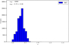 |
Fig. A.4 Same as Fig. 7, but with ~10 000 trials repeating the V -shape technique for the Massalia family. The mean of the distribution is centered at α = 0.73 ± 0.06 and the bin size in the histogram is 0.03. |
A.1.3 Misa(2)
The C-type Misa family has been noted to have a subfamily located within it (Milani et al. 2014; Nesvorný et al. 2015) that we will call Misa(2). The V -shape identification technique was applied to 427 asteroids belonging to the Misa(2) asteroid family as defined by Nesvorný et al. (2015). The ratio  at (ac, C, α) maximizes at (2.66 au, 7.75 × 10⁻⁶ au, ~0.86); it is shown in the top panel of Fig. A.6 and is ~8 standard deviations above the mean value of
  .
.
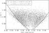 |
Fig. A.5 a
vs. |

The Monte Carlo tests have a mean value of α of ~0.87 ± 0.11 with positive skew as seen in Fig. 8. The family age of 120 ± 60 Myr is calculated using Eq. (22), with CYE = 5.5 × 10⁻⁶ au calculated from Eq. (20) where C = 7.75 × 10⁻⁶ au. The values of μα = 0.87 and CEV = 8.8 × 10⁻⁶ au are calculated using Eq. (19) assuming V EV = 12 m s-1, which is the escape speed of a 27 km diameter body with ρ = 1.4 g cm-3. We estimatethe D of the parent body of the Misa(2) family by using the technique of Tanga et al. (1999). The calculation was repeated using the same parameters except with α = 1.0 and C = 9.5 × 10⁻⁶ au, obtaining a value of 130 ± 60 Myr.
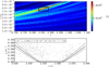 |
Fig. A.6 Same as Fig. 4, but for the Misa subfamily with data from Nesvorný et al. (2015). Top panel: Δα is equal to 5.0 × 10⁻³ au, and ΔC is equal to 1.3 × 10⁻⁶ au. Bottom panel: Dr(a, ac, C ± dC, pV, α) is plotted with pV = 0.1, ac = 2.655 au, and dC = 1.3 × 10⁻⁷ au. |
A.1.4 Tamara
The Tamara is a dark family of C-type asteroids located near the high i Phocaea region of the MB (Novaković et al. 2017). The V -shape identification technique was applied to 111 asteroids belonging to the Tamara asteroid family as defined by Novaković et al. (2017) with pV < 0.1. Only asteroids with known D measurements from Masiero et al. (2011) were used. Asteroid pV values were calculated with H values from Vereš et al. (2015) and D from Masiero et al. (2011) according to
 (A.1)
(A.1)
from Harris & Lagerros (2002). The interval [0.10, 0.58] for the Dirac delta function δ(Dr,j − Dr) is used and Eq. (12) is truncated to 0.10 km−1 for Dr < 0.10 km−1 and to 0.58 km−1 for Dr > 0.58 km−1. The peak in  at (ac, C, α) = (2.31 au, 1.7 × 10⁻⁵ au, ~0.79) is shown in the top panel of Fig. A.7 and is ~5 standard deviations above the mean. Approximately 1200 runs were performed with a mean value of α of ~0.70 ± 0.04 as seen in Fig. A.8.
The family age of 120 ± 60 Myr is calculated using Eq. (22), with CYE = 5.7 × 10⁻⁶ au calculated from Eq. (20) where C = 1.5 × 10⁻⁵ au. The value ofμα = 0.87 and CEV = 9.3 × 10⁻⁶ au are calculated using Eq. (19) assuming V EV = 46 m s-1, which is the escape speed of a 53 km diameter body with ρ = 1.4 g cm-3. We estimatethe D of the parent body of the Tamara family by using the technique of Tanga et al. (1999). The other parameters in Eq. (22) used to calculate the family age for Tamara are ac = 2.31 au, eμ = 0.2, ρmu = 1.4 g cm-3, pV = 0.06, and Gμ = 0.15. The calculation was repeated using the same parameters except with α = 1.0 and C = 2.3 × 10⁻⁵ au obtaining a value of 180 ± 90 Myr.
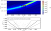 |
Fig. A.7 Same as Fig. 4, but for the Tamara asteroid family data from Novaković et al. (2017). Top panel: Δα is equal to 7.0 × 10⁻³ au, and ΔC is equal to 5.0 × 10⁻⁷ au. Bottom panel: Dr(a, ac, C ± dC, pV, α) is plotted with pV = 0.06, ac = 2.310 au, and dC = 7.0 × 10⁻⁶ au. |
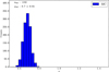 |
Fig. A.8 Same as Fig. 7, but with ~1200 trials repeating the V -shape technique for the Tamara family. The mean of the distribution is centered at α = 0.70 ± 0.04 and the bin size in the histogram is 0.03. |
A.2 Clipped V-shape families
A.2.1 Agnia
The S-type Agnia family is located in the central region of the MB bordering the 5:2 MMR with Jupiter (Zappalà et al. 1995) and contains subfamily Jitka (Milani et al. 2014). The V -shape identification technique was applied to 2123 asteroids belonging to the Agnia asteroid family as defined by Nesvorný et al. (2015). The interval [0.10, 1.32] for the Dirac delta function δ(Dr,j − Dr) is used and Eq. (12) is truncated to 0.10 km−1 for Dr < 0.10 km−1 and to 1.32 km−1 for Dr > 1.32 km−1. Asteroid H values were converted to D using Eq. (15) and a value of pV = 0.18 typical for members of the Agnia family (Masiero et al. 2013; Spoto et al. 2015). The peak in  at (ac, C, α) = (2.79 au, 1.54 × 10⁻⁵ au, ~0.91) is shown in the top panel of Fig. 9 and is ~3 standard deviations above the mean. The technique was repeated with the Agnia family defined by Milani et al. (2014) resulting in similar results to those seen in Fig. A.9. The Monte Carlo mean value of α is ~0.90 ± 0.03 as seen in Fig. A.10.
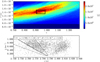 |
Fig. A.9 Same as Fig. 9, but repeated for the Agnia family defined by Milani et al. (2014). |
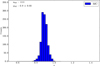 |
Fig. A.10 Same as Fig. 7, but with ~1100 trials repeating the V -shape technique for the Agnia family. The mean of the distribution is centered at α = 0.90 ± 0.03 and the bin size in the histogram is 0.02. |
The family age of 120 ± 60 Myr is calculated using Eq. (22), with CYE = 7.9 × 10⁻⁶ au calculated from Eq. (20) where C = 1.5 × 10⁻⁵ au and is similar to the 130 Myr age calcluated by Vokrouhlický et al. (2006b). The value of μα = 0.9 and CEV = 7.5 × 10⁻⁶ au are calculated using Eq. (19) assuming V EV = 15 m s-1 from (Vokrouhlický et al. 2006b). The calculation was repeated using the same parameters except with α = 1.0 and C = 1.8 × 10⁻⁵ obtaining a value of 100 ± 50 Myr.
A.2.2 Astrid
The C-type Astrid family is located in the central region of the MB and borders the 5:2 MMR with Jupiter (Zappalà et al. 1995). Members of the family interact with the s − sC nodal resonances with the asteroid Ceres affecting the distribution of its family members in a vs. sin i space (Carruba 2016). The interval [0.13, 0.67] for the Dirac delta function δ(Dr,j − Dr) is used and Eq. (12) is truncated to 0.13 km−1 for Dr < 0.13 km−1 and to 0.67 km−1 for Dr > 0.67 km−1. Asteroid H values were converted to D using Eq. (15) and a value of pV = 0.18 typical for members of the Astrid family (Masiero et al. 2013; Spoto et al. 2015). The peak in  at (ac, C, α) = (2.79 au, 1.28 × 10⁻⁵ au, ~ 0.86) is shown in the top panel of Fig. A.11 and is ~6 standard deviations above the mean value. The mean value of α from the Monte Carlo test is ~0.81 ± 0.07 as seen in Fig. A.11.
The family age of 110 ± 60 Myr is calculated using Eq. (22), with CYE = 3.9 × 10⁻⁶ au calculated from Eq. (20) where C = 1.2 × 10⁻⁵ au. This age is in agreement with the ~140 Myr age for the astrid family by (Carruba 2016). The value of μα = 0.81 and CEV = 8.1 × 10⁻⁶ au are calculated using Eq. (19) assuming V EV = 15 m s-1 from Vokrouhlický et al. (2006b).
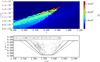 |
Fig. A.11 Same as Fig. 4, but for Astrid asteroid family data from Nesvorný et al. (2015). Top panel: Δα is equal to 1.5 × 10⁻² au, and ΔC is equal to 2.0 × 10⁻⁷ au. Bottom panel: Dr(a, ac, C ± dC, pV, α) is plotted with pV = 0.08, ac = 2.787 au, and dC = 3.2 × 10⁻⁶ au. |
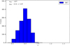 |
Fig. A.12 Same as Fig. 7, but with ~1300 trials repeating the V -shape technique for the Astrid family. The mean of the distribution is centered at α = 0.81 ± 0.07 and the bin size in the histogram is 0.06. |
A.2.3 Baptistina
The X-type Baptistina family is located in the inner region of the MB and borders the 7:2 /5:9 MMR with Jupiter/Mars (Knežević & Milani 2003; Mothé-Diniz et al. 2005; Bottke et al. 2007). The taxonomy of the Baptistina families may also be closer to S-types (Reddy et al. 2009, 2011). The V -shape identification technique was applied to 2450 asteroids belonging to the Baptistina asteroid family as defined by Nesvorný et al. (2015). The peak in  at (ac, C, α) = (2.26 au, 1.76 × 10⁻⁵ au, ~0.85) is shown in the top panel of Fig. A.13 and is ~5 standard deviations above the mean value. Approximately 2000 Monte Carlo runs were performed where the mean value of α is ~0.83 ± 0.05 as seen in Fig. A.14.
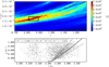 |
Fig. A.13 Same as Fig. 4, but for Baptistina asteroid family data from Nesvorný et al. (2015). Top panel: Δα is equal to 1.4 × 10⁻² au, and ΔC is equal to 6.0 × 10⁻⁷ au. Bottom panel: Dr(a, ac, C ± dC, pV, α) is plotted with pV = 0.16, ac = 2.262 au, and dC = 5.0 × 10⁻⁶ au. |
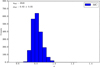 |
Fig. A.14 Same as Fig. 7, but with ~2000 trials repeating the V -shape technique for the Baptistina family. The mean of the distribution is centered at α = 0.83 ± 0.05 and the bin size in the histogram is 0.04. |
The family age of 200 ± 100 Myr is calculated using Eq. (22), with CYE = 1.0 × 10⁻⁵ au calculated from Eq. (20) where C = 1.76 × 10⁻⁵ au. The value ofμα = 0.83 and CEV = 7.6 × 10⁻⁶ au are calculated using Eq. (19) assuming V EV = 21 m s-1 from (Brož & Morbidelli 2013).
A.2.4 Dora(2)
The C-type Dora located in the central region of the MB contains a subfamily with a clipped V -shape (Nesvorný et al. 2015) that we will call Dora(2); it borders the 5:2 MMR with Jupiter. The V -shape identification technique was applied to 1223 asteroids belonging to the Dora asteroid family as defined by Nesvorný et al. (2015). The peak in  at (ac, C, α) = (2.8 au, 9.8 × 10⁻⁵ au, ~0.87) for the Dora(2) subfamily is shown in the top panel of Fig. A.15 and is ~4 standard deviations above the mean value. The mean value of α in the Monte Carlo trials is ~0.86 ± 0.04 as seen in Fig. A.16.
V -shapes with (ac, C, α) = (2.8 au, 9.8 × 10⁻⁶ au, 0.86) and (ac, C, α) = (2.8 au, 1.3 × 10⁻⁵ au, 1.0) according to Eq. (12) are overplotted on the V -shape with α = 1.0, which was obtained by repeating the V -shape technique with the fixed value of α = 1.0. The Dora(2)family V -shape is better fit with α = 0.86 than the V -shape with α = 1.0 as seen in Fig. A.17.
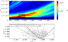 |
Fig. A.15 Same as Fig. 4, but for the Dora asteroid family data from Nesvorný et al. (2015). Top panel: Δα is equal to 1.4 × 10⁻² au, and ΔC is equal to 6.0 × 10⁻⁷ au. Bottom panel: Dr(a, ac, C ± dC, pV, α) is plotted with pV = 0.05, ac = 2.796 au, and dC = 7.5 × 10⁻⁶ au. |
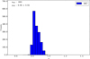 |
Fig. A.16 Same as Fig. 7, but with ~1600 trials repeating the V -shape technique for the Dora(2) family. The mean of the distribution is centered at α = 0.86 ± 0.04 and the bin size in the histogram is 0.03. |
The family age of 100 ± 50 Myr is calculated using Eq. (22), with CYE = 5.8 × 10⁻⁶ au calculated from Eq. (20) where C = 9.8 × 10⁻⁶ au. The value ofμα = 0.86 and CEV = 4.0 × 10⁻⁶ au are calculated using Eq. (19) assuming V EV = 15 m s-1, which is the escape speed of a 27 km diameter body with ρ = 1.4 g cm-3.
A.2.5 Eos
The K-type Eos family is located in the outer region of the MB, and is bracketed by the 7:3 and 11:5 MMR and the z1 resonance, and bisected by the 9:4 MMR with Jupiter, respectively (Hirayama 1918; Zappalà et al. 1990; Carruba & Michtchenko 2007; Brož & Morbidelli 2013). The V -shape identification technique was applied to 6897 asteroids belonging to the Eos asteroid family as defined by Nesvorný et al. (2015). The interval [0.04, 0.34] for the Dirac delta function δ(Dr,j − Dr) is used and Eq. (12) is truncated to 0.05 km−1 for Dr < 0.05 km−1 and to 0.34 km−1 for Dr > 0.34 km−1. The lower bound on including objects with Dr < 0.05 excludes objects that have not had their original spin axes modified by the YORP effect over the age of the Eos family (Hanuš et al. 2018). Asteroid H values were converted to D using Eq. (15) and a value of pV = 0.13 typical for members of the Eos family (Masiero et al. 2013; Spoto et al. 2015).
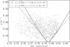 |
Fig. A.17 a
vs. |

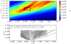 |
Fig. A.18 Same as Fig. 4, but for Eos asteroid family data from Nesvorný et al. (2015). Top panel: Δα is equal to 6.0 × 10⁻³ au, and ΔC is equal to 2.5 × 10⁻⁶ au. Bottom panel: Dr(a, ac, C ± dC, pV, α) is plotted with pV = 0.13, ac = 3.024 au, and dC = 5.0 × 10⁻⁵ au. |
The peak in  at (ac, C, α) = (3.02 au, 1.28 × 10⁻⁴ au, ~0.91) is shown in the top panel of Fig. A.18 and is ~3 standard deviations above the mean value. The mean value of α in the Monte Carlo trials is ~0.92 ± 0.02 as seen in Fig. A.18.
The family age of 1.08 ± 0.54 Gyr iscalculated using Eq. (23), with CYE = 9.3 × 10⁻⁵ au calculated from Eq. (20) where C = 1.3 × 10⁻⁴ au, which is similar to the ~1.3 Gyr age given by (Vokrouhlický et al. 2006c). The value of μα = 0.92 and CEV = 3.4 × 10⁻⁵ au are calculated using Eq. (19) assuming V EV = 70 m s-1 from (Nesvorný et al. 2015). The other parameters in Eq. (22) used to calculate the family age for Eos are ac = 3.024 au, eμ = 0.07, ρmu = 2.3 g cm-3, pV = 0.13, and Gμ = 0.24. The calculation was repeated using the same parameters except with α = 1.0 and C = 1.5 × 10⁻⁴ obtaining a value of 1.13± 0.56 Gyr.
A.2.6 Eunomia
The S-type Eunomia family is located in the central region of the MB and is bracketed by the 3:1 and 8:3 MMRs with Jupiter (Zappalà et al. 1990). The V -shape identification technique was applied to 1311 asteroids belonging to the Eunomia asteroid family as defined by Nesvorný et al. (2015). The interval [0.05, 0.21] for the Dirac delta function δ(Dr,j − Dr) is used and Eq. (12) is truncated to 0.05 km−1 for Dr< 0.05 km−1 and to 0.21 km−1 for Dr > 0.21 km−1. Asteroid H values were converted to D using Eq. (15) and a value of pV = 0.19 typical for members of the Eunomia family (Masiero et al. 2013; Spoto et al. 2015).
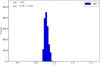 |
Fig. A.19 Same as Fig. 7, but with ~1500 trials repeating the V -shape technique for the Eos family. The mean of the distribution is centered at α = 0.92 ± 0.02 and the bin size in the histogram is 0.02. |
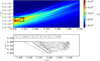 |
Fig. A.20 Same as Fig. 4, but for Eunomia asteroid family data from Nesvorný et al. (2015). Top panel: Δα is equal to 3.0 × 10⁻³ au, and ΔC is equal to 2.0 × 10⁻⁶ au. Bottom panel: Dr(a, ac, C ± dC, pV, α) is plotted with pV = 0.19, ac = 2.635 au, and dC = 5.0 × 10⁻⁵ au. |
The peak in  at (ac, C, α) = (2.64 au, 1.48 × 10⁻⁴ au, ~0.83) is shown in the top panel of Fig. A.20 and is ~5 standard deviations above the mean value. There were ~1700 Monte Carlo runs where the mean value of α is ~0.77 ± 0.03 as seen in Fig. A.21.
The family age of 1.1 ± 0.83 Gyr iscalculated using Eq. (23), with CYE = 5.9 × 10⁻⁵ au calculated from Eq. (20) where C = 1.32 × 10⁻⁴ au and overlaps with the 1.6–2.7 Gyr age found by Carruba et al. (2016c). The value of μα= 0.77 and CEV = 7.3 × 10⁻⁵ au are calculated using Eq. (19) assuming V EV = 15 m s-1, which is the escape speed of a 276 km diameter body with ρ = 2.3 g cm-3.
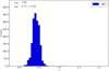 |
Fig. A.21 Same as Fig. 7 with ~1700 trials repeating the V -shape technique for the Eunomia family. The mean of the distribution is centered at α = 0.77 ± 0.03 and the bin size in the histogram is 0.02. |
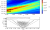 |
Fig. A.22 Same as Fig. 4, but for for Hoffmeister asteroid family data from Nesvorný et al. (2015). Top panel: Δα is equal to 3.5 × 10⁻³ au, and ΔC is equal to 3.5 × 10⁻⁷ au. Bottom panel: Dr(a, ac, C ± dC, pV, α) is plotted with pV = 0.04, ac = 2.785 au, and dC = 6.0 × 10⁻⁶ au. |
A.2.7 Hoffmeister
The C-type Hoffmeister family is located in the central region of the MB bracketed between the 3:1:1 three-body resonance with Jupiter and Saturn at 2.752 au and 5:2 MMR with Jupiter at 2.82 au and interacts with the s-sC nodal resonance with Ceres (Zappalà et al. 1995; Novaković et al. 2015; Carruba et al. 2017a). The V -shape identification technique was applied to 1773 asteroids belonging to the Hoffmeister asteroid family as defined by Nesvorný et al. (2015). The peak in  at (ac, C, α) = (2.79 au, 1.92 × 10⁻⁵ au, ~0.86) is shown inthe top panel of Fig. A.22 and is ~4 standard deviations above the mean value. Approximately ~1500 Monte Carlo runs were completed by randomizing H magnitudes by 0.25 and pV values were assumed to be 0.04 with an uncertainty of 0.01 with a mean value of α of ~0.84 ± 0.03 as seen in Fig. A.23.
The family age of 220 ± 110 Myr is calculated using Eq. (22), with CYE = 1.0 × 10⁻⁵ au calculated from Eq. (20) where C = 1.5 × 10⁻⁵ au and is in agreement with the ageof ~220 Myr for the Hoffmeister given by Carruba et al. (2017a). The value of μα= 0.84 and CEV = 4.7 × 10⁻⁶ au are calculated using Eq. (19) assuming V EV = 20 m s-1 from Carruba et al. (2017a).
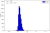 |
Fig. A.23 Same as Fig. 7, but with ~1500 trials repeating the V -shape technique for the Hoffmeister family. The mean of the distribution is centered at α = 0.84 ± 0.03 and the bin size in the histogram is 0.01. |
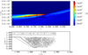 |
Fig. A.24 Same as Fig. 4, but for Hungaria asteroid family data from Nesvorný et al. (2015). Top panel: Δα is equal to 3.5 × 10⁻³ au, and ΔC is equal to 1.7 × 10⁻⁷ au. Bottom panel: Dr(a, ac, C ± dC, pV, α) is plotted with pV = 0.35, ac = 1.9425 au, and dC = 7.5 × 10⁻⁶ au. |
A.2.8 Hungaria
The E-type Hungaria family is located interior to the inner region of the MB and is bracketed by numerous secular resonances within 1.87 au and the 4:1 MMR with Jupiter at 2.06 au (Warner et al. 2009; Milani & Gronchi 2010). The V -shape identification technique was applied to 2337 asteroids belonging to the Hungaria asteroid family as defined by Nesvorný et al. (2015). The interval [0.28, 1.22] for the Dirac delta function δ(Dr,j − Dr) is used and Eq. (12) is truncated to 0.28 km−1 for Dr< 0.28 km−1 and to 1.23 km−1 for Dr> 1.23 km−1. Asteroid H values were converted to D using Eq. (15) and a value of pV = 0.35 typical for members of the Hungaria family (Shepard et al. 2008; Spoto et al. 2015).
The peak in  at (ac, C, α) = (1.94 au, 3.1 × 10⁻⁵ au, ~0.8) is shown in the top panel of Fig. A.24 and is ~7 standard deviations above the mean value. Approximately 2000 Monte Carlo runs were completed with a mean value of α of ~0.90 ± 0.03 as seen in Fig. A.25.
The family age of 300 ± 150 Myr is calculated using Eq. (22), with CYE = 2.1 × 10⁻⁵ au calculated from Eq. (20) where C = 3.1 × 10⁻⁵ au. The value ofμα = 0.79 and CEV = 1.0 × 10⁻⁵ au calculated using Eq. (19) assuming V EV = 25 m s-1, which is the escape speed of a 41.4 km diameter body with ρ = 2.7 g cm-3.
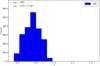 |
Fig. A.25 Same as Fig. 7, but with ~2000 trials repeating the V -shape technique for the Hungaria family. The mean of the distribution is centered at α = 0.79 ± 0.09 and the bin size in the histogram is 0.06. |
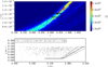 |
Fig. A.26 Same as Fig. 4, but for Hygiea asteroid family data from Nesvorný et al. (2015). Top panel: Δα is equal to 6.5 × 10⁻³ au, and ΔC is equal to 2.5 × 10⁻⁶ au. Bottom panel: Dr(a, ac, C ± dC, pV, α) is plotted with pV = 0.06, ac = 3.157 au, and dC = 2.0 × 10⁻⁵ au. |
A.2.9 Hygiea
The C-type Hygiea family is located in the outer region of the MB and borders the 9:4 MMR with Jupiter (Zappalà et al. 1995; Carruba et al. 2014). The V -shape identification technique was applied to 553 asteroids belonging to the Hygiea asteroid family as defined by Nesvorný et al. (2015). The peak in  at (ac, C, α) = (3.16 au, 1.175 × 10⁻⁴ au, ~0.93) is shown in the top panel of Fig. A.26 and is ~8 standard deviations above the mean value. There were ~2350 Monte Carloruns with a mean value of α of ~0.92 ± 0.02 as seen in Fig. A.27.
The family age of 0.92 ± 0.46 Gyr iscalculated using Eq. (23), with CYE = 5.2 × 10⁻⁵ au calculated from Eq. (20) where C = 1.2 × 10⁻⁵ au; however,as discussed by Carruba et al. (2014), this age may be an upper limit as Hygiea can perturb its members which affects their a. The value of μα= 0.92 and CEV = 6.5 × 10⁻⁵ au are calculated using Eq. (19) assuming V EV = 190 m s-1 from Vokrouhlický et al. (2006b). The calculation was repeated using the same parameters except with α = 1.0 and C = 1.4 × 10⁻⁴ obtaining a value of 1.2 ± 0.58 Gyr.
 |
Fig. A.27 Same as Fig. 7, but with ~2400 trials repeating the V -shape technique for the Hygiea family. The mean of the distribution is centered at α = 0.92 ± 0.02 and the bin size in the histogram is 0.01. |
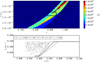 |
Fig. A.28 Same as Fig. 4, but for Koronis asteroid family data from Nesvorný et al. (2015). Top panel: Δα is equal to 3.5 × 10⁻³ au, and ΔC is equal to 1.5 × 10⁻⁶ au. Bottom panel: Dr(a, ac, C ± dC, pV, α) is plotted with pV = 0.15, ac = 2.883 au, and dC = 3.5 × 10⁻⁵ au. |
A.2.10 Koronis
The S-type Koronis family is located in the outer region of the MB and is bracketed by the 5:2 and 7:3 MMRs with Jupiter (Hirayama 1918; Zappalà et al. 1995; Bottke et al. 2001). The V -shape identification technique was applied to 516 asteroids belonging to the Koronis asteroid family as defined by Nesvorný et al. (2015). The peak in  at (ac, C, α) = (2.88 au, 1.53 × 10⁻⁴ au, ~0.91) is shown in the top panel of Fig. A.28 and is ~3 standard deviations above the mean value. Approximately 2700 Monte Carlo runs were completed with a mean value of α of ~0.93 ± 0.03 as seen in Fig. A.29.
The family age of 1.94 ± 0.97 Gyr iscalculated using Eq. (23), with CYE = 1.1 × 10⁻⁴ au calculated from Eq. (20) where C = 1.52 × 10⁻⁴ au and overlaps with the age estimate of ~2.4 Gyr for Koronis family given by Carruba et al. (2016c). The value of μα= 0.93 and CEV = 4.30 × 10⁻⁵ au are calculated using Eq. (19) assuming V EV = 90 m s-1, which is the escape speed of a 160 km diameter body with ρ = 2.3 g cm-3. This is similar to the estimate of V EV = 80 m s-1 by Carruba et al. (2016b) based on the e and i distribution of its family members.
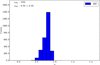 |
Fig. A.29 Same as Fig. 7, but with ~2700 trials repeating the V -shape technique for the Koronis family. The mean of the distribution is centered at α = 0.93 ± 0.03 and the bin size in the histogram is 0.04. |
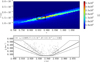 |
Fig. A.30 Same as Fig. 4, but for Naema asteroid family data from Nesvorný et al. (2015). Top panel: Δα is equal to 7.0 × 10⁻³ au, and ΔC is equal to 5.0 × 10⁻⁷ au. Bottom panel: Dr(a, ac, C ± dC, pV, α) is plotted with pV = 0.08, ac = 2.939 au, and dC = 5.0 × 10⁻⁶ au. |
A.2.11 Naema
The C-type Naema family is located in the outer region of the MB (Zappalà et al. 1995). The V -shape identification technique was applied to 281 asteroids belonging to the Naema asteroid family as defined by Nesvorný et al. (2015). The peak in  at (ac, C, α) = (2.94 au, 1.5 × 10⁻⁵ au, ~0.87) is shown in the top panel of Fig. A.30 and is ~7 standard deviations above the mean value. Approximately 1600 Monte Carlo runs were completed with a mean value of α of ~0.81 ± 0.05 as seen in Fig. A.31.
The family age of 40 ± 20 Myr is calculated using Eq. (22), with CYE = 2.4 × 10⁻⁶ au calculated from Eq. (20) where C = 1.5 × 10⁻⁵ au.
A.2.12 Padua
The C-type Padua family is located in the central region of the MB and is bracketed by the 8:3 MMR with Jupiter at 2.705 au and the 3:1:1 three-body resonance with Jupiter and Saturn at 2.752 au with Jupiter and Saturn (Carruba 2009). The V -shape identification technique was applied to 558 asteroids belonging to the Padua asteroid family as defined by Nesvorný et al. (2015). The peak in  at (ac, C, α) = (2.746 au, 3.8 × 10⁻⁵ au, ~ 0.89) is shown in the top panel of Fig. A.32 and is ~10 standard deviations above the mean value. There were ~1000 Monte Carloruns with a mean value of α of ~0.90 ± 0.11 and is positively skewed as seen in Fig. A.33.
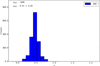 |
Fig. A.31 Same as Fig. 7, but with ~1600 trials repeating the V -shape technique for the Naema family. The mean of the distribution is centered at α = 0.81 ± 0.05 and the bin size in the histogram is 0.04. |
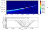 |
Fig. A.32 Same as Fig. 4, but for Padua asteroid family data from Nesvorný et al. (2015). Top panel: Δα is equal to 1.0 × 10⁻² au, and ΔC is equal to 1.0 × 10⁻⁶ au. Bottom panel: Dr(a, ac, C ± dC, pV, α) is plotted with pV = 0.24, ac = 2.744 au, and dC = 8.0 × 10⁻⁶ au. |
The family age of 310 ± 160 Myr is calculated using Eq. (22), with CYE = 2.5 × 10⁻⁵ au calculated from Eq. (20) where C = 3.8 × 10⁻⁵ au. The value ofμα = 0.89 and CEV = 1.3 × 10⁻⁵ au are calculated using Eq. (19) assuming V EV = 15 m s-1 from Vokrouhlický et al. (2006a). This value is considerably lower than the V EV = 30 m s-1 described by Carruba (2009) and could be due to the lack of information regarding the size of the original parent body of the Padua family causing V EV to be underestimated.
A.3 Half V-shape families
A.3.1 Adeona
The C-type Adeona family is located in the central region of the MB and borders the 3:8 resonance with Jupiter (Zappalà et al. 1995; Carruba et al. 2003). The V -shape identification technique was applied to 2152 asteroids belonging to the Adeona asteroid family as defined by Nesvorný et al. (2015). The peak in  at (ac, C, α) = (2.71 au, 1.0 × 10⁻⁵ au, ~0.91) is shown in the top panel of Fig. A.34 and is ~4 standard deviations above the mean value; the ranges 2.5 au < a < 2.75 au, 0.5 × 10⁻⁵ au < C < 12.0 × 10⁻⁴ au, and 0.8 < α < 1.1. A d C = 3.0 × 10⁻⁵ au were used. There were ~1600 runs with the mean value of α of ~0.83 ± 0.03 as seen in Fig. A.35.
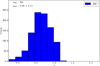 |
Fig. A.33 Same as Fig. 7, but with ~1000 trials repeating the V -shape technique for the Padua family. The mean of the distribution is centered at α = 0.89 ± 0.11 and the bin size in the histogram is 0.07. |
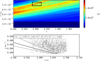 |
Fig. A.34 Same as Fig. 4, but for Adeona asteroid family data from Nesvorný et al. (2015). Top panel: Δα is equal to 3.5 × 10⁻³ au, and ΔC is equal to 1.4 × 10⁻⁶ au. Bottom panel: Dr(a, ac, C ± dC, pV, α) is plotted with pV = 0.07, ac = 2.705 au, and dC = 3.0 × 10⁻⁵ au. |
The family age of 1.4 ± 0.7 Gyr is calculated using Eq. (23), with CYE = 7.2 × 10⁻⁵ au calculated from Eq. (20) where C = 1.0 × 10⁻⁵ au. The value ofμα = 0.83 and CEV = 2.3 × 10⁻⁵ au are calculated using Eq. (19) assuming V EV = 78 m s-1 from Vokrouhlický et al. (2006b).
A.3.2 Eulalia
The C-type Eulalia family is located in the inner region of the MB and borders the 3:1 resonance with Jupiter (Walsh et al. 2013). The V -shape identification technique was applied to 2123 asteroids belonging to the Nysa-Polana asteroid family as defined by Nesvorný et al. (2015). The interval [0.04, 0.49] for the Dirac delta function δ(Dr,j − Dr) is used and Eq. (12) is truncated to 0.04 km−1 for Dr< 0.04 km−1 and to 0.49 km−1 for Dr > 0.49 km−1. Asteroid H values were converted to D using Eq. (15) and a value of pV = 0.06 typical for members of the Eulalia family (Walsh et al. 2013). The peak in  at (ac, C, α) = (2.49 au, 6.15 × 10⁻⁵ au, ~0.78) is ~3 standard deviations above the mean value. Approximately 2100 Monte Carlo runs were completed with a mean value of α of ~0.78 ± 0.06 and is positively skewed as seen in Fig. A.36. The Eulalia family V -shape is better fit with α = 0.78 than the V -shape with α = 1.0 as seen in Fig. A.37.
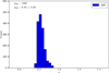 |
Fig. A.35 Same as Fig. 7, but with ~1600 trials repeating the V -shape technique for the Adeona family. The mean of the distribution is centered at α = 0.83 ± 0.03 and the bin size in the histogram is 0.01. |
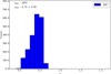 |
Fig. A.36 Same as Fig. 7, but with ~2100 trials repeating the V -shape technique for the Eulalia family. The mean of the distribution is centered at α = 0.78 ± 0.06 and the bin size in the histogram is 0.04. |
The family age of 840 ± 420 Myr is calculated using Eq. (22), with CYE = 4.8 × 10⁻⁶ au calculated from Eq. (20) where C = 6.5 × 10⁻⁵ au. The value ofμα = 0.78 and CEV = 1.4 × 10⁻⁶ au are calculated using Eq. (19) assuming V EV = 58 m s-1, which is the escape speed of a 130 km diameter body with ρ = 1.4 g cm-3.
A.3.3 Flora
The S-type Flora family is located in the inner region of the MB and borders the ν6 resonance with Saturn at ~2.16 au and is bisected by the 7:2 /5:9 MMR with Jupiter/Mars (Hirayama 1922; Zappalà et al. 1990; Dykhuis et al. 2014). The V -shape identification technique was applied to 5362 asteroids belonging to the Flora asteroid family as defined by Nesvorný et al. (2015). The peak in  at (ac, C, α) = (2.2 au, 1.27 × 10⁻⁴ au, ~0.77) is shown in the top panel of Fig. A.38 and is ~5 standard deviations above the mean value. Approximately 2000 Monte Carlo runs were completed with the mean value of α of ~0.83 ± 0.06 as seen in Fig. A.39.
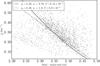 |
Fig. A.37 a
vs. |

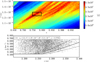 |
Fig. A.38 Same as Fig. 4, but for Flora asteroid family data from Nesvorný et al. (2015). Top panel: Δα is equal to 7.0 × 10⁻³ au, and ΔC is equal to 4.0 × 10⁻⁶ au. Bottom panel: Dr(a, ac, C ± dC, pV, α) is plotted with pV = 0.29, ac = 2.20 au, and dC = 3.2 × 10⁻⁵ au. |
The family age of 1.16 ± 0.58 Gyr iscalculated using Eq. (23), with CYE = 8.75 × 10⁻⁵ au calculated from Eq. (20) where C = 1.27 × 10⁻⁴ au. This is in agreement with the lower bound on age of a 1–1.4 Gyr family by Vokrouhlický et al. (2017a), but as noted in their paper, the upper bound on the family’s age is more compatible with the surface age of the asteroid Gaspara. We will have to consider ourfamily age estimate on the lower bound of the acceptable ages constrained by the surface age of Gaspara. The value of μα = 0.83 and CEV = 3.9 × 10⁻⁵ au are calculated using Eq. (19) assuming V EV = 87 m s-1, which is the escape speed of a 155 km diameter body with ρ = 2.3 g cm-3.
A.3.4 Maria
The S-type Maria family is located in the central region of the MB and borders the 3:1 MMR with jupiter (Hirayama 1922; Zappalà et al. 1990). The V -shape identification technique was applied to 1144 asteroids belonging to the Maria asteroid family as defined by Nesvorný et al. (2015). The peak in  at (ac, C, α) = (2.584 au, 1.1 × 10⁻⁴ au, ~0.9) is shown in the top panel of Fig. A.40 and is ~5 standard deviations above the mean. The technique was repeated with the Maria family defined by Milani et al. (2014) resulting in similar results as seen in Fig. A.41. Approximately 1800 Monte Carlo runs were completed with a mean of α of ~0.87 ± 0.03 as seen in Fig. A.42. The Maria family V -shape is better fit with α = 0.87 than the V -shape with α = 1.0 as seen in Fig. A.43.
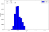 |
Fig. A.39 Same as Fig. 7, but with ~2000 trials repeating the V -shape technique for the Flora family. The mean of the distribution is centered at α = 0.83 ± 0.06 and the bin size in the histogram is 0.04. |
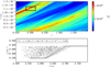 |
Fig. A.40 Same as Fig. 4, but for Maria asteroid family data from Nesvorný et al. (2015). Top panel: Δα is equal to 1.5 × 10⁻³ au, and ΔC is equal to 8.0 × 10⁻⁷ au. Bottom panel: Dr(a, ac, C ± dC, pV, α) is plotted with pV = 0.25, ac = 2.584 au, and dC = 1.5 × 10⁻⁵ au. |
The family age of 1.16 ± 0.58 Gyr iscalculated using Eq. (23), with CYE = 6.5 × 10⁻⁵ au calculated from Eq. (20) where C = 1.1 × 10⁻⁴ au, in agreement with the results of (Aljbaae et al. 2017a) for the age of the Maria family. The value of μα= 0.87 and CEV = 4.6 × 10⁻⁵ au are calculated using Eq. (19) assuming V EV = 65 m s-1, which is the escape speed of a 116 km diameter body with ρ = 2.3 g cm-3.
A.3.5 Nemausa
The inner main belt contains a low albedo asteroid family with an age ~4 Gyr that borders the 3:1 MMR with Jupiter that we will call the Nemausa family (Delbo’ et al. 2017). The V -shape identification technique was applied to 3949 asteroids with 0.0< e < 0.35, 0.0° < i < 14.5° and 0.0 < pV < 0.12. Only asteroids with known D measurements from Masiero et al. (2011) were used. Asteroid pV values were calculated with H values from Vereš et al. (2015) and D from Masiero et al. (2011) according to Eq. (A.1). The peak in  at (ac, C, α) = (2.386 au, 2.95 × 10⁻⁴ au, ~0.9) is shown in the top panel of Fig. A.44 and is ~10 standard deviations above the mean. Approximately 1500 Monte Carlo runs were completed with the mean value of α of ~0.92 ± 0.03 as seen in Fig. A.45.
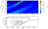 |
Fig. A.41 Milani Maria family. |
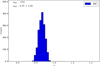 |
Fig. A.42 Same as Fig. 7, but with ~1800 trials repeating the V -shape technique for the Maria family. The mean of the distribution is centered at α = 0.87 ± 0.03 and the bin size in the histogram is 0.02. |
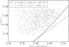 |
Fig. A.43 a
vs. |

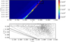 |
Fig. A.44 Same as Fig. 4, but for Nemausa asteroid family data from Nesvorný et al. (2015). Top panel: Δα is equal to 4.0 × 10⁻³ au, and ΔC is equal to 2.5 × 10⁻⁶ au. Bottom panel: Dr(a, ac, C ± dC, pV, α) is plotted with pV = 0.05, ac = 2.37 au, and dC = 5.0 × 10⁻⁵ au. |
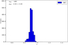 |
Fig. A.45 Same as Fig. 7, but with ~1500 trials repeating the V -shape technique for the Nemausa family. The mean of the distribution is centered at α = 0.92 ± 0.03 and the bin size in the histogram is 0.02. |
The family age of 4.3 ± 2.1 Gyr is calculated using Eq. (23), with CYE = 2.81 × 10⁻⁴ au calculated from Eq. (20) where C = 2.95 × 10⁻⁴ au. The value ofμα = 0.92 and CEV = 1.40 × 10⁻⁵ au are calculated using Eq. (19) assuming V EV = 60 m s-1, which is the escape speed of a 140 km diameter body with ρ = 1.4 g cm-3.
A.3.6 Nemesis
The C-type Nemesis family is located in the central region of the MB (Bendjoya & Zappalà 2002). Family fragments in the outer V -shape half are depleted as a result of possible close encounters with Ceres (Spoto et al. 2015). In addition, the nodal resonance between Nemsis family members and Ceres may play an important role in dynamically sculpting the asteroid family (Novaković et al. 2015). The V -shape identification technique was applied to 1250 asteroids belonging to the Nemesis asteroid family as defined by Nesvorný et al. (2015). The peak in  at (ac, C, α) = (2.738 au, 1.28 × 10⁻⁵ au, ~0.856) is shown in the top panel of Fig. A.46 and is ~3 standard deviations above the mean. Approximately 1600 Monte Carlo runs were completed with the mean value of α of ~0.8 ± 0.03 as seen in Fig. A.47.
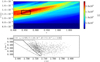 |
Fig. A.46 Same as Fig. 4, but for Nemesis asteroid family data from Nesvorný et al. (2015). Top panel: Δα is equal to 3.5 × 10⁻³ au, and ΔC is equal to 1.5 × 10⁻⁷ au. Bottom panel: Dr(a, ac, C ± dC, pV, α) is plotted with pV = 0.05, ac = 2.738 au, and dC = 7.5 × 10⁻⁶ au. |
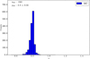 |
Fig. A.47 Same as Fig. 7, but with ~1600 trials repeating the V -shape technique for the Nemesis family. The mean of the distribution is centered at α = 0.80 ± 0.03 and the bin size in the histogram is 0.02. |
The family age of 150 ± 80 Myr is calculated using Eq. (22), with CYE = 9.5 × 10⁻⁶ au calculated from Eq. (20) where C = 1.3 × 10⁻⁵ au. The value ofμα = 0.8 and CEV = 3.3 × 10⁻⁶ au are calculated using Eq. (19) assuming V EV = 12.8 m s-1, which is the escape speed of a 29 km diameter body with ρ = 1.4 g cm-3.
A.3.7 New Polana
The C-type New Polana family is located in the inner region of the MB and overlaps the 3:1 resonance with Jupiter (Walsh et al. 2013). The V -shape identification technique was applied to 1818 asteroids belonging to the Nysa-Polana asteroid family as defined by Nesvorný et al. (2015). The peak in  at (ac, C, α) = (2.43 au, 1.23 × 10⁻⁴ au, ~0.82) is shown in the top panel of Fig. A.48 and is ~9 standard deviations above the mean value. There were ~2300 Monte Carloruns with a mean value of α of ~0.79 ± 0.06 as seen in Fig. A.49. The New Polana family V -shape is better fit with α = 0.83 than the V -shape with α = 1.0 as seen in Fig. A.50.
The family age of 2.1 ± 1.0 Gyr is calculated using Eq. (23), with CYE = 1.1 × 10⁻⁴ au calculated from Eq. (20) where C = 1.2 × 10⁻⁵ au. The value ofμα = 0.79 and CEV = 1.3 × 10⁻⁵ au are calculated using Eq. (19) assuming V EV = 57 m s-1, which is the escape speed of a 130 km diameter body with ρ = 1.4 g cm-3. The calculation was repeated using the same parameters except with α = 1.0 and C = 2.0 × 10⁻⁴ obtaining a value of 2.6 ± 1.3 Gyr.
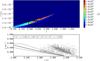 |
Fig. A.48 Same as Fig. 4, but for New Polana asteroid family data from Nesvorný et al. (2015). Top panel: Δα is equal to 2.7 × 10⁻³ au, and ΔC is equal to 2.5 × 10⁻⁶ au. Bottom panel: Dr(a, ac, C ± dC, pV, α) is plotted with pV = 0.06, ac = 2.426 au, and dC = 2.7 × 10⁻⁵ au. |
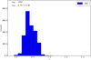 |
Fig. A.49 Same as Fig. 7, but with ~2300 trials repeating the V -shape technique for the New Polana family. The mean of the distribution is centered at α = 0.79 ± 0.06 and the bin size in the histogram is 0.05. |
 |
Fig. A.50 a
vs. |

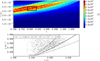 |
Fig. A.51 Same as Fig. 4, but for Rafita asteroid family data from Nesvorný et al. (2015). Top panel: Δα is equal to 8.1 × 10⁻³ au, and ΔC is equal to 2.5 × 10⁻⁶ au. Bottom panel: Dr(a, ac, C ± dC, pV, α) is plotted with pV = 0.25, ac = 2.549 au, and dC = 1.7 × 10⁻⁵ au. |
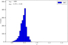 |
Fig. A.52 Same as Fig. 7, but with ~1900 trials repeating the V -shape technique for the Rafita family. The mean of the distribution is centered at α = 0.79 ± 0.05 and the bin size in the histogram is 0.02. |
A.3.8 Rafita
The S-type Rafita family is located in the central region of the MB and borders the 3:1 MMR with Jupiter (Zappalà et al. 1990). The V -shape identification technique was applied to 1251 asteroids belonging to the Rafita asteroid family as defined by Nesvorný et al. (2015). The interval [0.10, 1.32] for the Dirac delta function δ(Dr,j − Dr) is used and Eq. (12) is truncated to 0.06 km−1 for Dr < 0.06 km−1 and to 1.71 km−1 for Dr > 1.71 km−1. Asteroid H values were converted to D using Eq. (15) and a value of pV = 0.25 typical for members of the Rafita family (Masiero et al. 2013; Spoto et al. 2015). The peak in  at (ac, C, α) = (2.549 au, 4.6 × 10⁻⁵ au, ~0.81) is shown in the top panel of Fig. A.51 and is ~3 standard deviations above the mean. Approximately 1900 Monte Carlo runs were completed with a mean value of α of ~0.79 ± 0.05 as seen in Fig. A.52. The Rafita family V -shape is better fit with α = 0.79 than the V -shape with α = 1.0 as seen in Fig. A.53.
The family age of 380 ± 190 Myr is calculated using Eq. (22), with CYE = 4.0 × 10⁻⁵ au calculated from Eq. (20) where C = 4.6 × 10⁻⁵ au which overlaps with the 300–700 Myr estimate of (Aljbaae et al. 2017b). The value of μα= 0.79 and CEV = 6.1 × 10⁻⁶ au are calculated using Eq. (19) assuming V EV = 12 m s-1, which is the escape speed of a 27 km diameter body with ρ = 1.4 g cm-3.
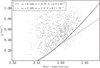 |
Fig. A.53 a
vs. |

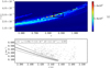 |
Fig. A.54 Same as Fig. 4, but for Sulamitis asteroid family data from Nesvorný et al. (2015). Top panel: Δα is equal to 1.3 × 10⁻² au, and ΔC is equal to 1.0 × 10⁻⁶ au. Bottom panel: Dr(a, ac, C ± dC, pV, α) is plotted with pV = 0.04, ac = 2.472 au, and dC = 5.0 × 10⁻⁶ au. |
A.3.9 Sulamitis
The C-type Sulamitis family is located in the inner region of the MB and borders the 3:1 resonance with Jupiter (Zappalà et al. 1995). The V -shape identification technique was applied to 284 asteroids belonging to the Sulamitis asteroid family as defined by Nesvorný et al. (2015). The peak in  at (ac, C, α) = (2.472 au, 3.0 × 10⁻⁵ au, ~0.875) is shown in the top panel of Fig. A.54 and is ~11 standard deviations above the mean value. There were ~2200 Monte Carloruns with a mean value of α of ~0.87 ± 0.02 as seen in Fig. A.55. The family age of 470 ± 230 Myr is calculated using Eq. (22), with CYE = 2.4 × 10⁻⁵ au calculated from Eq. (20) where C = 3.0 × 10⁻⁵ au.
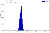 |
Fig. A.55 Same as Fig. 7, but with ~2200 trials repeating the V -shape technique for the Sulamitis family. The mean of the distribution is centered at α = 0.87 ± 0.02 and the bin size in the histogram is 0.01. |
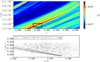 |
Fig. A.56 Same as Fig. 4, but for Ursula asteroid family data from Nesvorný et al. (2015). Top panel: Δα is equal to 2.1 × 10⁻³ au, and ΔC is equal to 6.0 × 10⁻⁷ au. Bottom panel: Dr(a, ac, C ± dC, pV, α) is plotted with pV = 0.06, ac = 3.218 au, and dC = 2.0 × 10⁻⁵ au. |
 |
Fig. A.57 Same as Fig. 7, but with ~2300 trials repeating the V -shape technique for the Ursula family. The mean of the distribution is centered at α = 0.90 ± 0.02 and the bin size in the histogram is 0.01. |
A.3.10 Ursula
The C-type Ursula family is located in the outer region of the MB and borders the 2:1 MMR with Jupiter at 3.2 au (Zappalà et al. 1995). The V -shape identification technique was applied to 1209 asteroids belonging to the Ursula asteroid family as defined by Nesvorný et al. (2015). The interval [0.03, 0.24] for the Dirac delta function δ(Dr,j − Dr) is used and Eq. (12) is truncated to 0.03 km−1 for Dr < 0.03 km−1 and to 0.24 km−1 for Dr > 0.24 km−1. Asteroid H values were converted to D using Eq. (15) and a value of pV = 0.06 typical for members of the Ursula family (Masiero et al. 2013; Spoto et al. 2015). The peak in  at (ac, C, α) = (2.79 au, 1.54 × 10⁻⁵ au, ~0.91) is shown in the top panel of Fig. A.56 and is ~6 standard deviations above the mean. ~2374 with a meanvalue of α of ~0.90 ± 0.02 as seen in Fig. A.57. The family age of 2.3 ± 1.1 Gyr is calculated using Eq. (23), with CYE = 1.2 × 10⁻⁴ au calculated from Eq. (20) where C = 1.6 × 10⁻⁴ au and overlaps with the estimate from Carruba et al. (2016c) of 1 ~4 Gyr.
Acknowledgements
We would like to thank the reviewer of our manuscript, Valerio Carruba, for providing helpful comments and suggestions for improving the quality of the text. B. T. Bolin is supported by l’École Doctorale Sciences Fondatementales et Appliquées, ED.SFA (ED 364) at l’Université de Nice-Sophia Antipolis. K. J. Walsh was supported by the National Science Foundation, Grant 1518127. B. T. B. would like to acknowledge J. W. Westover for thought-provoking discussions on the implementation of large-scale computing resources and algorithms that were used in the completion of this work.
References
- Alí-Lagoa, V., Lionni, L., Delbo, M., et al. 2014, A&A, 561, A45 [NASA ADS] [CrossRef] [EDP Sciences] [Google Scholar]
- Aljbaae, S., Carruba, V., Masiero, J. R., Domingos, R. C., & Huaman, M. 2017a, MNRAS, 471, 4820 [NASA ADS] [CrossRef] [Google Scholar]
- Aljbaae, S., Carruba, V., Masiero, J. R., Domingos, R. C., & Huaman, M. 2017b, MNRAS, 467, 1016 [NASA ADS] [Google Scholar]
- Bendjoya, P., & Zappalà, V. 2002, Asteroids III, 613 [Google Scholar]
- Bertotti, B., Farinella, P., & Vokrouhlick, D. 2003, Physics of the Solar System – Dynamics and Evolution, Space Physics, and Spacetime Structure, Astrophys. Space Sci. Lib., 293 [Google Scholar]
- Boggs, P. T., & Rogers, J. E. 1990, Statistical analysis of measurement error models and applications: proceedings of the AMS-IMS-SIAM joint summer research conference held June 10–16, 1989, 112, 186 [Google Scholar]
- Bolin, B. T., Delbo, M., Morbidelli, A., & Walsh, K. J. 2017a, Icarus, 282, 290 [NASA ADS] [CrossRef] [Google Scholar]
- Bolin, B. T., Walsh, K. J., Morbidelli, A., & Delbo, M. 2017b, MNRAS, 473, 3949 [NASA ADS] [CrossRef] [Google Scholar]
- Bottke, Jr. W. F., Rubincam, D. P., & Burns, J. A. 2000, Icarus, 145, 301 [NASA ADS] [CrossRef] [Google Scholar]
- Bottke, W. F., Vokrouhlický, D., Brož, M., Nesvorný, D., & Morbidelli, A. 2001, Science, 294, 1693 [NASA ADS] [CrossRef] [PubMed] [Google Scholar]
- Bottke, Jr. W. F., Vokrouhlický, D., Rubincam, D. P., & Brož, M. 2002, Asteroids III, 395 [Google Scholar]
- Bottke, W. F., Durda, D. D., Nesvorný, D., et al. 2005, Icarus, 179, 63 [NASA ADS] [CrossRef] [Google Scholar]
- Bottke, Jr. W. F., Vokrouhlický, D., Rubincam, D. P., & Nesvorný, D. 2006, Ann. Rev. Earth Planet. Sci., 34, 157 [Google Scholar]
- Bottke, W. F., Vokrouhlický, D., & Nesvorný, D. 2007, Nature, 449, 48 [NASA ADS] [CrossRef] [Google Scholar]
- Bottke, W. F., Vokrouhlický, D., Walsh, K. J., et al. 2015, Icarus, 247, 191 [NASA ADS] [CrossRef] [Google Scholar]
- Bowell, E., Hapke, B., Domingue, D., et al. 1988, Asteroids II, 399 [Google Scholar]
- Brož, M., & Morbidelli, A. 2013, Icarus, 223, 844 [NASA ADS] [CrossRef] [Google Scholar]
- Brož, M., Morbidelli, A., Bottke, W. F., et al. 2013, A&A, 551, A117 [NASA ADS] [CrossRef] [EDP Sciences] [Google Scholar]
- Carruba, V. 2009, MNRAS, 395, 358 [NASA ADS] [CrossRef] [Google Scholar]
- Carruba, V. 2016, MNRAS, 461, 1605 [NASA ADS] [CrossRef] [Google Scholar]
- Carruba, V., & Michtchenko, T. A. 2007, A&A, 475, 1145 [NASA ADS] [CrossRef] [EDP Sciences] [Google Scholar]
- Carruba, V., & Nesvorný, D. 2016, MNRAS, 457, 1332 [NASA ADS] [CrossRef] [Google Scholar]
- Carruba, V., Burns, J. A., Bottke, W., & Nesvorný, D. 2003, Icarus, 162, 308 [NASA ADS] [CrossRef] [Google Scholar]
- Carruba, V., Domingos, R. C., Huaman, M. E., Santos, C. R. d., & Souami, D. 2014, MNRAS, 437, 2279 [NASA ADS] [CrossRef] [Google Scholar]
- Carruba, V., Aljbaae, S., & Winter, O. C. 2016a, MNRAS, 455, 2279 [NASA ADS] [CrossRef] [Google Scholar]
- Carruba, V., Nesvorný, D., & Aljbaae, S. 2016b, Icarus, 271, 57 [NASA ADS] [CrossRef] [Google Scholar]
- Carruba, V., Nesvorný, D., Aljbaae, S., Domingos, R. C., & Huaman, M. 2016c, MNRAS, 458, 3731 [NASA ADS] [CrossRef] [Google Scholar]
- Carruba, V., Novaković, B., & Aljbaae, S. 2017a, MNRAS, 465, 4099 [NASA ADS] [CrossRef] [Google Scholar]
- Carruba, V., Vokrouhlický, D., & Nesvorný, D. 2017b, MNRAS, 469, 4400 [NASA ADS] [CrossRef] [Google Scholar]
- Carry, B. 2012, Planet. Space Sci., 73, 98 [NASA ADS] [CrossRef] [Google Scholar]
- Carry, B., Matter, A., Scheirich, P., et al. 2015, Icarus, 248, 516 [NASA ADS] [CrossRef] [Google Scholar]
- Cellino, A., Michel, P., Tanga, P., et al. 1999, Icarus, 141, 79 [NASA ADS] [CrossRef] [Google Scholar]
- Chesley, S. R., Farnocchia, D., Nolan, M. C., et al. 2014, Icarus, 235, 5 [NASA ADS] [CrossRef] [Google Scholar]
- Consolmagno, G., Britt, D., & Macke, R. 2008, Chemie der Erde/Geochemistry, 68, 1 [Google Scholar]
- Cotto-Figueroa, D., Statler, T. S., Richardson, D. C., & Tanga, P. 2015, ApJ, 803, 25 [NASA ADS] [CrossRef] [Google Scholar]
- Delbo, M., & Tanga, P. 2009, Planet. Space Sci., 57, 259 [NASA ADS] [CrossRef] [Google Scholar]
- Delbó, M., Harris, A. W., Binzel, R. P., Pravec, P., & Davies, J. K. 2003, Icarus, 166, 116 [NASA ADS] [CrossRef] [Google Scholar]
- Delbo, M., dell’Oro, A., Harris, A. W., Mottola, S., & Mueller, M. 2007, Icarus, 190, 236 [NASA ADS] [CrossRef] [Google Scholar]
- Delbo, M., Libourel, G., Wilkerson, J., et al. 2014, Nature, 508, 233 [NASA ADS] [CrossRef] [Google Scholar]
- Delbo, M., Mueller, M., Emery, J. P., Rozitis, B., & Capria, M. T. 2015, Asteroids IV, 107 [Google Scholar]
- Delbo’, M., Walsh, K., Bolin, B., Avdellidou, C., & Morbidelli, A. 2017, Science, 357, 1026 [NASA ADS] [CrossRef] [Google Scholar]
- Drummond, J. D., Conrad, A., Merline, W. J., et al. 2010, A&A, 523, A93 [NASA ADS] [CrossRef] [EDP Sciences] [Google Scholar]
- Durda, D. D., Bottke, W. F., Nesvorný, D., et al. 2007, Icarus, 186, 498 [NASA ADS] [CrossRef] [Google Scholar]
- Dykhuis, M. J., Molnar, L., Van Kooten, S. J., & Greenberg, R. 2014, Icarus, 243, 111 [NASA ADS] [CrossRef] [Google Scholar]
- Emery, J. P., Fernández, Y. R., Kelley, M. S. P., et al. 2014, Icarus, 234, 17 [NASA ADS] [CrossRef] [Google Scholar]
- Farinella, P., Vokrouhlický, D., & Hartmann, W. K. 1998, Icarus, 132, 378 [NASA ADS] [CrossRef] [Google Scholar]
- Fujiwara, A., Kawaguchi, J., Yeomans, D. K., et al. 2006, Science, 312, 1330 [NASA ADS] [CrossRef] [PubMed] [Google Scholar]
- Greenberg, A. H., Margot, J.-L., Verma, A. K., Taylor, P. A., & Hodge, S. E. 2017, ArXiv e-prints [arxiv:1708.05513] [Google Scholar]
- Grogan, K., Dermott, S. F., & Durda, D. D. 2001, Icarus, 152, 251 [NASA ADS] [CrossRef] [Google Scholar]
- Gundlach, B., & Blum, J. 2012, Icarus, 219, 618 [NASA ADS] [CrossRef] [EDP Sciences] [Google Scholar]
- Gundlach, B., & Blum, J. 2013, Icarus, 223, 479 [NASA ADS] [CrossRef] [Google Scholar]
- Hanuš, J., Delbo’, M., Ďurech, J., & Alí-Lagoa, V. 2015, Icarus, 256, 101 [NASA ADS] [CrossRef] [Google Scholar]
- Hanuš, J., Delbo’, M., Vokrouhlický, D., et al. 2016, A&A, 592, A34 [NASA ADS] [CrossRef] [EDP Sciences] [Google Scholar]
- Hanuš, J., Marchis, F., Viikinkoski, M., Yang, B., & Kaasalainen, M. 2017, A&A, 599, A36 [NASA ADS] [CrossRef] [EDP Sciences] [Google Scholar]
- Hanuš, J., Delbo’, M., Alí-Lagoa, V., et al. 2018, Icarus, 299, 84 [NASA ADS] [CrossRef] [Google Scholar]
- Harris, A., & Drube, L. 2016, in AAS/Division for Planetary Sciences Meeting Abstracts, 48, 516.05 [NASA ADS] [Google Scholar]
- Harris, A. W., & Lagerros, J. S. V. 2002, Asteroids III, 205 [Google Scholar]
- Hirayama, K. 1918, AJ, 31, 185 [NASA ADS] [CrossRef] [Google Scholar]
- Hirayama, K. 1922, Japanese J. Astron. Geophys., 1, 55 [NASA ADS] [Google Scholar]
- Horz, F., & Cintala, M. 1997, Meteor. Planet. Sci., 32 [Google Scholar]
- Jedicke, R., & Metcalfe, T. S. 1998, Icarus, 131, 245 [NASA ADS] [CrossRef] [Google Scholar]
- Jedicke, R., Larsen, J., & Spahr, T. 2002, Asteroids III, 71 [Google Scholar]
- Jedicke, R., Nesvorný, D., Whiteley, R., Ivezić, Ž., & Jurić, M. 2004, Nature, 429, 275 [NASA ADS] [CrossRef] [PubMed] [Google Scholar]
- Jedicke, R., Granvik, M., Micheli, M., et al. 2015, Surveys, Astrometric Follow-Up, and Population Statistics, eds. P. Michel, F. E. DeMeo, & W. F. Bottke, 795 [Google Scholar]
- Knežević, Z., & Milani, A. 2003, A&A, 403, 1165 [NASA ADS] [CrossRef] [EDP Sciences] [Google Scholar]
- Lamy, P. L., Kaasalainen, M., Lowry, S., et al. 2008, A&A, 487, 1179 [NASA ADS] [CrossRef] [EDP Sciences] [Google Scholar]
- Levison, H. F., & Duncan, M. J. 1994, Icarus, 108, 18 [NASA ADS] [CrossRef] [Google Scholar]
- Lowry, S. C., Weissman, P. R., Duddy, S. R., et al. 2014, A&A, 562, A48 [NASA ADS] [CrossRef] [EDP Sciences] [Google Scholar]
- Marchis, F., Enriquez, J. E., Emery, J. P., et al. 2012, Icarus, 221, 1130 [NASA ADS] [CrossRef] [Google Scholar]
- Margot, J.-L., Pravec, P., Taylor, P., Carry, B., & Jacobson, S. 2015, Asteroid Systems: Binaries, Triples, and Pairs, eds. P. Michel, F. E. DeMeo, & W. F. Bottke, 355 [Google Scholar]
- Masiero, J. R., Mainzer, A. K., Grav, T., et al. 2011, ApJ, 741, 68 [NASA ADS] [CrossRef] [Google Scholar]
- Masiero, J. R., Mainzer, A. K., Bauer, J. M., et al. 2013, ApJ, 770, 7 [NASA ADS] [CrossRef] [Google Scholar]
- Masiero, J. R., DeMeo, F. E., Kasuga, T., & Parker, A. H. 2015, Asteroids IV, 323 [Google Scholar]
- McMahon, J. W. 2017, in AAS/Division for Planetary Sciences Meeting Abstracts, 49, 111.09 [NASA ADS] [Google Scholar]
- Michel, P., Benz, W., Tanga, P., & Richardson, D. C. 2001, Science, 294, 1696 [NASA ADS] [CrossRef] [PubMed] [Google Scholar]
- Michel, P., Benz, W., & Richardson, D. C. 2004, Icarus, 168, 420 [NASA ADS] [CrossRef] [Google Scholar]
- Michel, P., Richardson, D. C., Durda, D. D., Jutzi, M., & Asphaug, E. 2015, Asteroids IV, 341 [Google Scholar]
- Milani, A., & Gronchi, G. F. 2010, Theory of Orbital Determination (Cambridge University Press) [Google Scholar]
- Milani, A., Cellino, A., Knezević, Z., et al. 2014, Icarus, 239, 46 [NASA ADS] [CrossRef] [Google Scholar]
- Milani, A., Knežević, Z., Spoto, F., et al. 2017, Icarus, 288, 240 [NASA ADS] [CrossRef] [Google Scholar]
- Mothé-Diniz, T., Roig, F., & Carvano, J. M. 2005, Icarus, 174, 54 [NASA ADS] [CrossRef] [Google Scholar]
- Mueller, M. 2012, ArXiv e-prints [arxiv:1208.3993] [Google Scholar]
- Müller, T. G., Ďurech, J., Hasegawa, S., et al. 2011, A&A, 525, A145 [NASA ADS] [CrossRef] [EDP Sciences] [Google Scholar]
- Müller, T. G., O’Rourke, L., Barucci, A. M., et al. 2012, A&A, 548, A36 [NASA ADS] [CrossRef] [EDP Sciences] [Google Scholar]
- Müller, T. G., Miyata, T., Kiss, C., et al. 2013, A&A, 558, A97 [NASA ADS] [CrossRef] [EDP Sciences] [Google Scholar]
- Müller, T. G., Hasegawa, S., & Usui, F. 2014a, PASJ, 66, 52 [NASA ADS] [CrossRef] [Google Scholar]
- Müller, T. G., Kiss, C., Scheirich, P., et al. 2014b, A&A, 566, A22 [NASA ADS] [CrossRef] [EDP Sciences] [Google Scholar]
- Naidu, S. P., Margot, J. L., Taylor, P. A., et al. 2015, AJ, 150, 54 [NASA ADS] [CrossRef] [Google Scholar]
- Nesvorný, D., Bottke, Jr. W. F., Dones, L., & Levison, H. F. 2002, Nature, 417, 720 [NASA ADS] [CrossRef] [Google Scholar]
- Nesvorný, D., Bottke, W. F., Levison, H. F., & Dones, L. 2003, ApJ, 591, 486 [NASA ADS] [CrossRef] [Google Scholar]
- Nesvorný, D., Enke, B. L., Bottke, W. F., et al. 2006, Icarus, 183, 296 [NASA ADS] [CrossRef] [Google Scholar]
- Nesvorný, D., Brož, M., & Carruba, V. 2015, Asteroids IV, 297 [Google Scholar]
- Novaković, B., Maurel, C., Tsirvoulis, G., & Knežević Z. 2015, ApJ, 807, L5 [NASA ADS] [CrossRef] [Google Scholar]
- Novaković, B., Tsirvoulis, G., Granvik, M., & Todović, A. 2017, AJ, 153, 266 [NASA ADS] [CrossRef] [Google Scholar]
- Oszkiewicz, D. A., Muinonen, K., Bowell, E., et al. 2011, J. Quant. Spectr. Rad. Transf., 112, 1919 [NASA ADS] [CrossRef] [Google Scholar]
- Paolicchi, P., & Knežević Z. 2016, Icarus, 274, 314 [NASA ADS] [CrossRef] [Google Scholar]
- Peterson, C. 1976, Icarus, 29, 91 [NASA ADS] [CrossRef] [Google Scholar]
- Pravec, P., & Harris, A. W. 2007, Icarus, 190, 250 [CrossRef] [Google Scholar]
- Pravec, P., Harris, A. W., & Michalowski, T. 2002, Asteroid Rotations, eds. W. F. Bottke, Jr. A. Cellino, P. Paolicchi, & R. P. Binzel, 113 [Google Scholar]
- Pravec, P., Harris, A. W., Kušnirák, P., Galád, A., & Hornoch, K. 2012, Icarus, 221, 365 [NASA ADS] [CrossRef] [Google Scholar]
- Radović, V., Novaković, B., Carruba, V., & Marčeta D. 2017, MNRAS, 470, 576 [NASA ADS] [CrossRef] [Google Scholar]
- Reddy, V., Emery, J. P., Gaffey, M. J., et al. 2009, Meteor. Planet. Sci., 44, 1917 [NASA ADS] [CrossRef] [Google Scholar]
- Reddy, V., Carvano, J. M., Lazzaro, D., et al. 2011, Icarus, 216, 184 [NASA ADS] [CrossRef] [Google Scholar]
- Rozitis, B., & Green, S. F. 2014, A&A, 568, A43 [NASA ADS] [CrossRef] [EDP Sciences] [Google Scholar]
- Rubincam, D. P. 1995, J. Geophys. Res., 100, 1585 [NASA ADS] [CrossRef] [Google Scholar]
- Shepard, M. K., Kressler, K. M., Clark, B. E., et al. 2008, Icarus, 195, 220 [NASA ADS] [CrossRef] [Google Scholar]
- Spitale, J., & Greenberg, R. 2002, Icarus, 156, 211 [NASA ADS] [CrossRef] [Google Scholar]
- Spoto, F., Milani, A., & Knežević Z. 2015, Icarus, 257, 275 [NASA ADS] [CrossRef] [Google Scholar]
- Statler, T. S. 2009, Icarus, 202, 502 [NASA ADS] [CrossRef] [Google Scholar]
- Tanga, P., Cellino, A., Michel, P., et al. 1999, Icarus, 141, 65 [NASA ADS] [CrossRef] [Google Scholar]
- Vereš, P., Jedicke, R., Fitzsimmons, A., et al. 2015, Icarus, 261, 34 [NASA ADS] [CrossRef] [Google Scholar]
- Vernazza, P., Binzel, R. P., Rossi, A., Fulchignoni, M., & Birlan, M. 2009, Nature, 458, 993 [NASA ADS] [CrossRef] [Google Scholar]
- Veverka, J., Thomas, P. C., Robinson, M., et al. 2001, Science, 292, 484 [NASA ADS] [CrossRef] [Google Scholar]
- Vokrouhlicky, D. 1998, A&A, 335, 1093 [NASA ADS] [Google Scholar]
- Vokrouhlický, D. 1999, A&A, 344, 362 [NASA ADS] [Google Scholar]
- Vokrouhlický, D., Brož, M., Bottke, W. F., Nesvorný, D., & Morbidelli, A. 2006a, Icarus, 183, 349 [NASA ADS] [CrossRef] [Google Scholar]
- Vokrouhlický, D., Brož, M., Bottke, W. F., Nesvorný, D., & Morbidelli, A. 2006b, Icarus, 182, 118 [NASA ADS] [CrossRef] [Google Scholar]
- Vokrouhlický, D., Brož, M., Morbidelli, A., et al. 2006c, Icarus, 182, 92 [NASA ADS] [CrossRef] [Google Scholar]
- Vokrouhlický, D., Bottke, W. F., Chesley, S. R., Scheeres, D. J., & Statler, T. S. 2015, Asteroids IV, 509 [Google Scholar]
- Vokrouhlický, D., Bottke, W. F., & Nesvorný, D. 2017a, AJ, 153, 172 [NASA ADS] [CrossRef] [Google Scholar]
- Vokrouhlický, D., Pravec, P., Durech, J., et al. 2017b, A&A, 598, A91 [NASA ADS] [CrossRef] [EDP Sciences] [Google Scholar]
- Walsh, K. J., Delbó, M., Bottke, W. F., Vokrouhlický, D., & Lauretta, D. S. 2013, Icarus, 225, 283 [NASA ADS] [CrossRef] [Google Scholar]
- Warner, B. D., Harris, A. W., Vokrouhlický, D., Nesvorný, D., & Bottke, W. F. 2009, Icarus, 204, 172 [NASA ADS] [CrossRef] [Google Scholar]
- Wolters, S. D., Rozitis, B., Duddy, S. R., et al. 2011, MNRAS, 418, 1246 [NASA ADS] [CrossRef] [Google Scholar]
- Yano, H., Kubota, T., Miyamoto, H., et al. 2006, Science, 312, 1350 [NASA ADS] [CrossRef] [PubMed] [Google Scholar]
- Yeomans, D. K., Antreasian, P. G., Barriot, J.-P., et al. 2000, Science, 289, 2085 [NASA ADS] [CrossRef] [PubMed] [Google Scholar]
- Zappalà, V., Cellino, A., Farinella, P., & Knežević, Z. 1990, AJ, 100, 2030 [NASA ADS] [CrossRef] [Google Scholar]
- Zappalà, V., Bendjoya, P., Cellino, A., Farinella, P., & Froeschlé, C. 1995, Icarus, 116, 291 [NASA ADS] [CrossRef] [Google Scholar]
- Zappalà, V., Cellino, A., dell’Oro, A., & Paolicchi, P. 2002, Asteroids III, 619 [Google Scholar]
All Tables
All Figures
|
Fig. 1 D vs. Γ for near-Earth and main belt asteroids of S, C, B, X, and E types and dynamical classes with D < 100 km. The data arefit to the function y = a xb shown as the dark line using orthogonal distance regression (Boggs & Rogers 1990). Measurements of D and Γ are taken from Delbó et al. (2003), Lamy et al. (2008), Delbo & Tanga (2009), Masiero et al. (2011), Müller et al. (2011), Wolters et al. (2011), Marchis et al. (2012), Müller et al. (2012), Müller et al. (2013), Emery et al. (2014), Alí-Lagoa et al. (2014), Müller et al. (2014b), Rozitis & Green (2014), Hanuš et al. (2015), Naidu et al. (2015), Hanuš et al. (2016). |
| In the text | |
|
Fig. 2 Same as Fig. 1, but for near-Earth and main belt asteroids of S, C, B, X, and E types and dynamical classes with 0.5 km < D < 100 km. Measurements of D and Γ are taken from Delbó et al. (2003), Lamy et al. (2008), Delbo & Tanga (2009), Masiero et al. (2011), Müller et al. (2011), Wolters et al. (2011), Marchis et al. (2012), Rozitis & Green (2014), Hanuš et al. (2015,2016), Naidu et al. (2015). |
| In the text | |
|
Fig. 3 Two generic family V -shapes with ac= 2.37 au and C = 1.9 × 10⁻⁵ au and α = 0.8, 1.0. |
| In the text | |
|
Fig. 4 Application of the V -shape identification to synthetic asteroid family data at Time = 200 Myr. Top panel: the ratio of
|
| In the text | |
|
Fig. 5 Same as Fig. 4, but for the Erigone asteroid family data from Nesvorný et al. (2015). Top panel: Δα is equal to 1.8 × 10⁻³ au, and ΔC is equal to 9.0 × 10⁻⁸ au. Bottom panel: Dr(a, ac, C ± dC, pV, α) is plotted with pV = 0.05, ac = 2.796 au, and dC = 7.5 × 10⁻⁶ au. |
| In the text | |
|
Fig. 6 Same as Fig. 5, but repeated for the Erigone family defined by Milani et al. (2014). |
| In the text | |
|
Fig. 7 Histogram of α
located at the peak value of |
| In the text | |
|
Fig. 8 Same as Fig. 7, but for ~4400 trials repeating the V -shape technique for the Misa family. The mean of the distribution is centered at α = 0.87± 0.11 and the bin size in the histogram is 0.04. |
| In the text | |
|
Fig. 9 Same as Fig. 4, but for Agnia asteroid family data from Nesvorný et al. (2015). Top panel: Δα is equal to 1.4 × 10⁻² au, and ΔC is equal to 7.4 × 10⁻⁷ au. Bottom panel: Dr(a, ac, C ± dC, pV, α) is plotted with pV = 0.18, ac = 2.791 au, and dC = 7.5 × 10⁻⁶ au. |
| In the text | |
|
Fig. 10 Same as Fig. 4, but for the Eulalia asteroid family data from Nesvorný et al. (2015). Top panel: Δα is equal to 7.5 × 10⁻³ au, and ΔC is equal to 8.0 × 10⁻⁷ au. Bottom panel: Dr(a, ac, C ± dC, pV, α) is plotted with pV = 0.05, ac = 2.49 au, and dC = 3.2 × 10⁻⁶ au. |
| In the text | |
|
Fig. 11 ac vs. α vs. revised age for asteroid families of all taxonomies. The Eos asteroid family is labeled as an S-type in this plot. The data are fit to the function y = a x + b in ac vs. α space, which is shown as the dark line using orthogonal distance regression (Boggs & Rogers 1990). |
| In the text | |
|
Fig. 12 Age vs. α for asteroid families of all taxonomies. The data are fit to the function y = a log10(x) + b shown as the dark line using orthogonal distance regression (Boggs & Rogers 1990). |
| In the text | |
|
Fig. A.1 a
vs. |
| In the text | |
|
Fig. A.2 Same as Fig. 4, but for Massalia asteroid family data from Nesvorný et al. (2015). Top panel: Δα is equal to 1.8 × 10⁻³ au, and ΔC is equal to 5.0 × 10⁻⁷ au. Bottom panel: Dr(a, ac, C ± dC, pV, α) is plotted with pV = 0.24, ac = 2.41 au, and dC = 5.0 × 10⁻⁶ au. |
| In the text | |
|
Fig. A.3 Same as Fig. A.2, but repeated for the Massalia family defined by Milani et al. (2014). |
| In the text | |
|
Fig. A.4 Same as Fig. 7, but with ~10 000 trials repeating the V -shape technique for the Massalia family. The mean of the distribution is centered at α = 0.73 ± 0.06 and the bin size in the histogram is 0.03. |
| In the text | |
|
Fig. A.5 a
vs. |
| In the text | |
|
Fig. A.6 Same as Fig. 4, but for the Misa subfamily with data from Nesvorný et al. (2015). Top panel: Δα is equal to 5.0 × 10⁻³ au, and ΔC is equal to 1.3 × 10⁻⁶ au. Bottom panel: Dr(a, ac, C ± dC, pV, α) is plotted with pV = 0.1, ac = 2.655 au, and dC = 1.3 × 10⁻⁷ au. |
| In the text | |
|
Fig. A.7 Same as Fig. 4, but for the Tamara asteroid family data from Novaković et al. (2017). Top panel: Δα is equal to 7.0 × 10⁻³ au, and ΔC is equal to 5.0 × 10⁻⁷ au. Bottom panel: Dr(a, ac, C ± dC, pV, α) is plotted with pV = 0.06, ac = 2.310 au, and dC = 7.0 × 10⁻⁶ au. |
| In the text | |
|
Fig. A.8 Same as Fig. 7, but with ~1200 trials repeating the V -shape technique for the Tamara family. The mean of the distribution is centered at α = 0.70 ± 0.04 and the bin size in the histogram is 0.03. |
| In the text | |
|
Fig. A.9 Same as Fig. 9, but repeated for the Agnia family defined by Milani et al. (2014). |
| In the text | |
|
Fig. A.10 Same as Fig. 7, but with ~1100 trials repeating the V -shape technique for the Agnia family. The mean of the distribution is centered at α = 0.90 ± 0.03 and the bin size in the histogram is 0.02. |
| In the text | |
|
Fig. A.11 Same as Fig. 4, but for Astrid asteroid family data from Nesvorný et al. (2015). Top panel: Δα is equal to 1.5 × 10⁻² au, and ΔC is equal to 2.0 × 10⁻⁷ au. Bottom panel: Dr(a, ac, C ± dC, pV, α) is plotted with pV = 0.08, ac = 2.787 au, and dC = 3.2 × 10⁻⁶ au. |
| In the text | |
|
Fig. A.12 Same as Fig. 7, but with ~1300 trials repeating the V -shape technique for the Astrid family. The mean of the distribution is centered at α = 0.81 ± 0.07 and the bin size in the histogram is 0.06. |
| In the text | |
|
Fig. A.13 Same as Fig. 4, but for Baptistina asteroid family data from Nesvorný et al. (2015). Top panel: Δα is equal to 1.4 × 10⁻² au, and ΔC is equal to 6.0 × 10⁻⁷ au. Bottom panel: Dr(a, ac, C ± dC, pV, α) is plotted with pV = 0.16, ac = 2.262 au, and dC = 5.0 × 10⁻⁶ au. |
| In the text | |
|
Fig. A.14 Same as Fig. 7, but with ~2000 trials repeating the V -shape technique for the Baptistina family. The mean of the distribution is centered at α = 0.83 ± 0.05 and the bin size in the histogram is 0.04. |
| In the text | |
|
Fig. A.15 Same as Fig. 4, but for the Dora asteroid family data from Nesvorný et al. (2015). Top panel: Δα is equal to 1.4 × 10⁻² au, and ΔC is equal to 6.0 × 10⁻⁷ au. Bottom panel: Dr(a, ac, C ± dC, pV, α) is plotted with pV = 0.05, ac = 2.796 au, and dC = 7.5 × 10⁻⁶ au. |
| In the text | |
|
Fig. A.16 Same as Fig. 7, but with ~1600 trials repeating the V -shape technique for the Dora(2) family. The mean of the distribution is centered at α = 0.86 ± 0.04 and the bin size in the histogram is 0.03. |
| In the text | |
|
Fig. A.17 a
vs. |
| In the text | |
|
Fig. A.18 Same as Fig. 4, but for Eos asteroid family data from Nesvorný et al. (2015). Top panel: Δα is equal to 6.0 × 10⁻³ au, and ΔC is equal to 2.5 × 10⁻⁶ au. Bottom panel: Dr(a, ac, C ± dC, pV, α) is plotted with pV = 0.13, ac = 3.024 au, and dC = 5.0 × 10⁻⁵ au. |
| In the text | |
|
Fig. A.19 Same as Fig. 7, but with ~1500 trials repeating the V -shape technique for the Eos family. The mean of the distribution is centered at α = 0.92 ± 0.02 and the bin size in the histogram is 0.02. |
| In the text | |
|
Fig. A.20 Same as Fig. 4, but for Eunomia asteroid family data from Nesvorný et al. (2015). Top panel: Δα is equal to 3.0 × 10⁻³ au, and ΔC is equal to 2.0 × 10⁻⁶ au. Bottom panel: Dr(a, ac, C ± dC, pV, α) is plotted with pV = 0.19, ac = 2.635 au, and dC = 5.0 × 10⁻⁵ au. |
| In the text | |
|
Fig. A.21 Same as Fig. 7 with ~1700 trials repeating the V -shape technique for the Eunomia family. The mean of the distribution is centered at α = 0.77 ± 0.03 and the bin size in the histogram is 0.02. |
| In the text | |
|
Fig. A.22 Same as Fig. 4, but for for Hoffmeister asteroid family data from Nesvorný et al. (2015). Top panel: Δα is equal to 3.5 × 10⁻³ au, and ΔC is equal to 3.5 × 10⁻⁷ au. Bottom panel: Dr(a, ac, C ± dC, pV, α) is plotted with pV = 0.04, ac = 2.785 au, and dC = 6.0 × 10⁻⁶ au. |
| In the text | |
|
Fig. A.23 Same as Fig. 7, but with ~1500 trials repeating the V -shape technique for the Hoffmeister family. The mean of the distribution is centered at α = 0.84 ± 0.03 and the bin size in the histogram is 0.01. |
| In the text | |
|
Fig. A.24 Same as Fig. 4, but for Hungaria asteroid family data from Nesvorný et al. (2015). Top panel: Δα is equal to 3.5 × 10⁻³ au, and ΔC is equal to 1.7 × 10⁻⁷ au. Bottom panel: Dr(a, ac, C ± dC, pV, α) is plotted with pV = 0.35, ac = 1.9425 au, and dC = 7.5 × 10⁻⁶ au. |
| In the text | |
|
Fig. A.25 Same as Fig. 7, but with ~2000 trials repeating the V -shape technique for the Hungaria family. The mean of the distribution is centered at α = 0.79 ± 0.09 and the bin size in the histogram is 0.06. |
| In the text | |
|
Fig. A.26 Same as Fig. 4, but for Hygiea asteroid family data from Nesvorný et al. (2015). Top panel: Δα is equal to 6.5 × 10⁻³ au, and ΔC is equal to 2.5 × 10⁻⁶ au. Bottom panel: Dr(a, ac, C ± dC, pV, α) is plotted with pV = 0.06, ac = 3.157 au, and dC = 2.0 × 10⁻⁵ au. |
| In the text | |
|
Fig. A.27 Same as Fig. 7, but with ~2400 trials repeating the V -shape technique for the Hygiea family. The mean of the distribution is centered at α = 0.92 ± 0.02 and the bin size in the histogram is 0.01. |
| In the text | |
|
Fig. A.28 Same as Fig. 4, but for Koronis asteroid family data from Nesvorný et al. (2015). Top panel: Δα is equal to 3.5 × 10⁻³ au, and ΔC is equal to 1.5 × 10⁻⁶ au. Bottom panel: Dr(a, ac, C ± dC, pV, α) is plotted with pV = 0.15, ac = 2.883 au, and dC = 3.5 × 10⁻⁵ au. |
| In the text | |
|
Fig. A.29 Same as Fig. 7, but with ~2700 trials repeating the V -shape technique for the Koronis family. The mean of the distribution is centered at α = 0.93 ± 0.03 and the bin size in the histogram is 0.04. |
| In the text | |
|
Fig. A.30 Same as Fig. 4, but for Naema asteroid family data from Nesvorný et al. (2015). Top panel: Δα is equal to 7.0 × 10⁻³ au, and ΔC is equal to 5.0 × 10⁻⁷ au. Bottom panel: Dr(a, ac, C ± dC, pV, α) is plotted with pV = 0.08, ac = 2.939 au, and dC = 5.0 × 10⁻⁶ au. |
| In the text | |
|
Fig. A.31 Same as Fig. 7, but with ~1600 trials repeating the V -shape technique for the Naema family. The mean of the distribution is centered at α = 0.81 ± 0.05 and the bin size in the histogram is 0.04. |
| In the text | |
|
Fig. A.32 Same as Fig. 4, but for Padua asteroid family data from Nesvorný et al. (2015). Top panel: Δα is equal to 1.0 × 10⁻² au, and ΔC is equal to 1.0 × 10⁻⁶ au. Bottom panel: Dr(a, ac, C ± dC, pV, α) is plotted with pV = 0.24, ac = 2.744 au, and dC = 8.0 × 10⁻⁶ au. |
| In the text | |
|
Fig. A.33 Same as Fig. 7, but with ~1000 trials repeating the V -shape technique for the Padua family. The mean of the distribution is centered at α = 0.89 ± 0.11 and the bin size in the histogram is 0.07. |
| In the text | |
|
Fig. A.34 Same as Fig. 4, but for Adeona asteroid family data from Nesvorný et al. (2015). Top panel: Δα is equal to 3.5 × 10⁻³ au, and ΔC is equal to 1.4 × 10⁻⁶ au. Bottom panel: Dr(a, ac, C ± dC, pV, α) is plotted with pV = 0.07, ac = 2.705 au, and dC = 3.0 × 10⁻⁵ au. |
| In the text | |
|
Fig. A.35 Same as Fig. 7, but with ~1600 trials repeating the V -shape technique for the Adeona family. The mean of the distribution is centered at α = 0.83 ± 0.03 and the bin size in the histogram is 0.01. |
| In the text | |
|
Fig. A.36 Same as Fig. 7, but with ~2100 trials repeating the V -shape technique for the Eulalia family. The mean of the distribution is centered at α = 0.78 ± 0.06 and the bin size in the histogram is 0.04. |
| In the text | |
|
Fig. A.37 a
vs. |
| In the text | |
|
Fig. A.38 Same as Fig. 4, but for Flora asteroid family data from Nesvorný et al. (2015). Top panel: Δα is equal to 7.0 × 10⁻³ au, and ΔC is equal to 4.0 × 10⁻⁶ au. Bottom panel: Dr(a, ac, C ± dC, pV, α) is plotted with pV = 0.29, ac = 2.20 au, and dC = 3.2 × 10⁻⁵ au. |
| In the text | |
|
Fig. A.39 Same as Fig. 7, but with ~2000 trials repeating the V -shape technique for the Flora family. The mean of the distribution is centered at α = 0.83 ± 0.06 and the bin size in the histogram is 0.04. |
| In the text | |
|
Fig. A.40 Same as Fig. 4, but for Maria asteroid family data from Nesvorný et al. (2015). Top panel: Δα is equal to 1.5 × 10⁻³ au, and ΔC is equal to 8.0 × 10⁻⁷ au. Bottom panel: Dr(a, ac, C ± dC, pV, α) is plotted with pV = 0.25, ac = 2.584 au, and dC = 1.5 × 10⁻⁵ au. |
| In the text | |
|
Fig. A.41 Milani Maria family. |
| In the text | |
|
Fig. A.42 Same as Fig. 7, but with ~1800 trials repeating the V -shape technique for the Maria family. The mean of the distribution is centered at α = 0.87 ± 0.03 and the bin size in the histogram is 0.02. |
| In the text | |
|
Fig. A.43 a
vs. |
| In the text | |
|
Fig. A.44 Same as Fig. 4, but for Nemausa asteroid family data from Nesvorný et al. (2015). Top panel: Δα is equal to 4.0 × 10⁻³ au, and ΔC is equal to 2.5 × 10⁻⁶ au. Bottom panel: Dr(a, ac, C ± dC, pV, α) is plotted with pV = 0.05, ac = 2.37 au, and dC = 5.0 × 10⁻⁵ au. |
| In the text | |
|
Fig. A.45 Same as Fig. 7, but with ~1500 trials repeating the V -shape technique for the Nemausa family. The mean of the distribution is centered at α = 0.92 ± 0.03 and the bin size in the histogram is 0.02. |
| In the text | |
|
Fig. A.46 Same as Fig. 4, but for Nemesis asteroid family data from Nesvorný et al. (2015). Top panel: Δα is equal to 3.5 × 10⁻³ au, and ΔC is equal to 1.5 × 10⁻⁷ au. Bottom panel: Dr(a, ac, C ± dC, pV, α) is plotted with pV = 0.05, ac = 2.738 au, and dC = 7.5 × 10⁻⁶ au. |
| In the text | |
|
Fig. A.47 Same as Fig. 7, but with ~1600 trials repeating the V -shape technique for the Nemesis family. The mean of the distribution is centered at α = 0.80 ± 0.03 and the bin size in the histogram is 0.02. |
| In the text | |
|
Fig. A.48 Same as Fig. 4, but for New Polana asteroid family data from Nesvorný et al. (2015). Top panel: Δα is equal to 2.7 × 10⁻³ au, and ΔC is equal to 2.5 × 10⁻⁶ au. Bottom panel: Dr(a, ac, C ± dC, pV, α) is plotted with pV = 0.06, ac = 2.426 au, and dC = 2.7 × 10⁻⁵ au. |
| In the text | |
|
Fig. A.49 Same as Fig. 7, but with ~2300 trials repeating the V -shape technique for the New Polana family. The mean of the distribution is centered at α = 0.79 ± 0.06 and the bin size in the histogram is 0.05. |
| In the text | |
|
Fig. A.50 a
vs. |
| In the text | |
|
Fig. A.51 Same as Fig. 4, but for Rafita asteroid family data from Nesvorný et al. (2015). Top panel: Δα is equal to 8.1 × 10⁻³ au, and ΔC is equal to 2.5 × 10⁻⁶ au. Bottom panel: Dr(a, ac, C ± dC, pV, α) is plotted with pV = 0.25, ac = 2.549 au, and dC = 1.7 × 10⁻⁵ au. |
| In the text | |
|
Fig. A.52 Same as Fig. 7, but with ~1900 trials repeating the V -shape technique for the Rafita family. The mean of the distribution is centered at α = 0.79 ± 0.05 and the bin size in the histogram is 0.02. |
| In the text | |
|
Fig. A.53 a
vs. |
| In the text | |
|
Fig. A.54 Same as Fig. 4, but for Sulamitis asteroid family data from Nesvorný et al. (2015). Top panel: Δα is equal to 1.3 × 10⁻² au, and ΔC is equal to 1.0 × 10⁻⁶ au. Bottom panel: Dr(a, ac, C ± dC, pV, α) is plotted with pV = 0.04, ac = 2.472 au, and dC = 5.0 × 10⁻⁶ au. |
| In the text | |
|
Fig. A.55 Same as Fig. 7, but with ~2200 trials repeating the V -shape technique for the Sulamitis family. The mean of the distribution is centered at α = 0.87 ± 0.02 and the bin size in the histogram is 0.01. |
| In the text | |
|
Fig. A.56 Same as Fig. 4, but for Ursula asteroid family data from Nesvorný et al. (2015). Top panel: Δα is equal to 2.1 × 10⁻³ au, and ΔC is equal to 6.0 × 10⁻⁷ au. Bottom panel: Dr(a, ac, C ± dC, pV, α) is plotted with pV = 0.06, ac = 3.218 au, and dC = 2.0 × 10⁻⁵ au. |
| In the text | |
|
Fig. A.57 Same as Fig. 7, but with ~2300 trials repeating the V -shape technique for the Ursula family. The mean of the distribution is centered at α = 0.90 ± 0.02 and the bin size in the histogram is 0.01. |
| In the text | |
Current usage metrics show cumulative count of Article Views (full-text article views including HTML views, PDF and ePub downloads, according to the available data) and Abstracts Views on Vision4Press platform.
Data correspond to usage on the plateform after 2015. The current usage metrics is available 48-96 hours after online publication and is updated daily on week days.
Initial download of the metrics may take a while.