| Issue |
A&A
Volume 611, March 2018
|
|
|---|---|---|
| Article Number | A25 | |
| Number of page(s) | 38 | |
| Section | Extragalactic astronomy | |
| DOI | https://doi.org/10.1051/0004-6361/201731271 | |
| Published online | 20 March 2018 | |
An updated Type II supernova Hubble diagram★
1
Astrophysics Research Centre, School of Mathematics and Physics, Queen’s University Belfast,
Belfast
BT7 1NN, UK
e-mail: This email address is being protected from spambots. You need JavaScript enabled to view it.
2
Max-Planck-Institut für Astrophysik,
Karl-Schwarzschild-Str. 1,
85748
Garching-bei-München, Germany
3
ESO,
Karl-Schwarzschild-Strasse 2,
85748
Garching, Germany
4
Excellence Cluster Universe, Technische Universität München,
Boltzmannstrasse 2,
85748
Garching-bei-München,
Germany
5
Heidelberger Institut für Theoretische Studien,
Schloss-Wolfsbrunnenweg 35,
69118
Heidelberg, Germany
6
Zentrum für Astronomie der Universität Heidelberg, Institut für Theoretische Astrophysik,
Philosophenweg 12,
69120
Heidelberg, Germany
7
The Oskar Klein Centre & Department of Astronomy, Stockholm University, AlbaNova,
106 91
Stockholm, Sweden
8
GMTO Corporation,
465 N. Halstead St., Suite 250 Pasadena,
CA
91107, USA
9
Institute for Astronomy, University of Hawaii at Manoa,
2680 Woodlawn Drive,
Honolulu,
HI
96822, USA
10
Centre for Extragalactic Astronomy, Department of Physics, Durham University,
South Road,
Durham
DH1 3LE, UK
Received:
30
May
2017
Accepted:
9
October
2017
Abstract
We present photometry and spectroscopy of nine Type II-P/L supernovae (SNe) with redshifts in the 0.045 ≲ z ≲ 0.335 range, with a view to re-examining their utility as distance indicators. Specifically, we apply the expanding photosphere method (EPM) and the standardized candle method (SCM) to each target, and find that both methods yield distances that are in reasonable agreement with each other. The current record-holder for the highest-redshift spectroscopically confirmed supernova (SN) II-P is PS1-13bni (z = 0.335−0.012+0.009), and illustrates the promise of Type II SNe as cosmological tools. We updated existing EPM and SCM Hubble diagrams by adding our sample to those previously published. Within the context of Type II SN distance measuring techniques, we investigated two related questions. First, we explored the possibility of utilising spectral lines other than the traditionally used Fe iiλ5169 to infer the photospheric velocity of SN ejecta. Using local well-observed objects, we derive an epoch-dependent relation between the strong Balmer line and Fe iiλ5169 velocities that is applicable 30 to 40 days post-explosion. Motivated in part by the continuum of key observables such as rise time and decline rates exhibited from II-P to II-L SNe, we assessed the possibility of using Hubble-flow Type II-L SNe as distance indicators. These yield similar distances as the Type II-P SNe. Although these initial results are encouraging, a significantly larger sample of SNe II-L would be required to draw definitive conclusions.
Key words: supernovae: general / distance scale
Tables A.1, A.3, A.5, A.7, A.9, A.11, A.13, A.15 and A.17 are also available at the CDS via anonymous ftp to cdsarc.u-strasbg.fr (130.79.128.5) or via http://cdsarc.u-strasbg.fr/viz-bin/qcat?J/A+A/611/A25
© ESO 2018
1 Introduction
The past decades have been marked by an ongoing revolution in cosmology and distance estimation techniques. Following the astounding discovery that the Universe was expanding at an accelerating rate (Riess et al. 1998; Perlmutter et al. 1999), the quest to determine the precise value of the Hubble constant, H0, has inspired a host of new distance determination techniques, systematic improvements to old approaches, as well as large-scale focussed projects dedicated to improving the precision in the measurements of H0 in order to shed light on the constituents of the energy density of the Universe.
Already in the 1980s i.e., before the launch of the Hubble Space Telescope (HST), the measurement of the Hubble constant with an uncertainty of ≲10% was chosen as one of three HST “Key Projects”. Freedman et al. (2001) presented the final results of this endeavour. Using an array of secondary distance indicators, calibrated using Cepheid distances, they reported a value for H0 of 72 ± 8 km s−1 Mpc−1.
Galaxies for which distance estimates from multiple sources are available are crucial as anchors for the extragalactic distance scale. One example is NGC 4258, which has estimates for a geometric distance through mega masers (Humphreys et al. 2013), a Cepheid distance (e.g. Fiorentino et al. 2013), and a Type II-P supernova (SN) distance (Polshaw et al. 2015). NGC 4258 may therefore be a more suitable anchor galaxy than the Large Magellanic Cloud, which was used as the first rung on the distance ladder for a variety of distance estimation techniques (Riess et al. 2011a,b, and references therein).
Recently, the Planck Collaboration XIII (2016) presented the outcomes of observations of the cosmic microwave background, which enabled them to restrict the Hubble constant to H0 = 67.8 ± 0.9 km s−1 Mpc−1, corresponding to an uncertainty of only 1.3%.
In the latest update, Riess et al. (2016) combined both newly calibrated distance measurements of Cepheid stars and Type Ia SNe, to constrain the Hubble constant to only 2.4% as H0 = 73.0 ± 1.8 km s−1 Mpc−1.
While the uncertainties in H0 have decreased significantly over the years, a disagreement at the 2.0–2.5σ level between the values derived via SN Ia cosmology and measurements of the cosmic microwave background has emerged, reflecting a tension between local and global measurements of H0. Such a discrepancy could either imply unknown systematic uncertainties in the measurements of H0 or that current cosmological models have to be revised (e.g. Bennett et al. 2014). Nevertheless, Bennett et al. (2014) also maintain that the various estimates of H0 are not inconsistent with each other.
The Expanding Photosphere Method (EPM; Kirshner & Kwan 1974) and the Standardized Candle Method (SCM; Hamuy & Pinto 2002) and their more recent derivatives provide independent routes to H0 . On the most fundamental level, the EPM relies on the comparison of the angular size of an object with the ratio between its observed and theoretical flux, whereas the SCM uses the relation between the expansion velocities of SNe II-P during the plateau phase and its plateau luminosity to determine the distance. The EPM and SCM are subject to different systematics than the previously mentioned techniques and they have both undergone significant improvements from their original description (e.g. Wagoner 1981; Schmidt et al. 1994b; Eastman et al. 1996; Hamuy et al. 2001; Dessart & Hillier 2005; Gall et al. 2016 for the EPM or Nugent et al. 2006; Poznanski et al. 2009 for the SCM), aiming to reduce their systematic uncertainties. In particular, the EPM is independentof the cosmic distance ladder. Additionally, SNe II-Pare more common albeit less luminous than SNe Ia, and bear the potential to be observed in statistically significant numbers.
Several other methods have been proposed to either improve on EPM or reduce the observational effort, mostly spectroscopy, for distance determination with Type II SNe. The application of a single dilution factor for the black body radiation has been shown to be a clear limitation of EPM. The Spectral Expanding Atmosphere Method (SEAM; Mitchell et al. 2002; Baron et al. 2004; Dessart & Hillier 2006) attempts to establish the physical conditions in the SN through detailed spectral fitting. In this case, the emergent flux is determined through detailed model fitting for each spectral epoch. This method requires excellent spectral data, and has so far been applied only to the brightest and nearest supernovae (SNe 1987A and 1999em). Variants of the SCM include the photospheric magnitude method (Rodríguez et al. 2014) and the photometric candle method (de Jaeger et al. 2015, 2017b). These rely almost exclusively on photometry, and have been mostly developed to exploit the large SN samples that are expected to become available in future surveys. A separate approach has been taken by Pejcha & Prieto (2015), who combine all available photometric and spectroscopic information to generate best fit synthetic light curves, yielding parameters such as reddening and nickel mass in addition to a relative distance. This method requires exquisite observational data to function, and in particular, it depends on a good sampling of the light curve and the velocity evolution for many SNe. Although this method does not provide an independent distance zeropoint, it obtains very good relative distances. Thus it is clear that no single approach is equally applicable at all redshifts.
Schmidt et al. (1994a) considered Type II SNe out to cz ~ 5500 km s−1, and developed much of the EPM framework. In this study, we build upon our previous work (Gall et al. 2015, 2016) where we re-examined relativistic effects – specifically, the difference between “angular size” and “luminosity” distance – that come into play when applying the EPM to SNe at non-negligible redshifts, a subtlety that was neglected in previous studies. We re-derived the basic equations of the EPM, and showed that for distant SNe, the angular size, θ, should be corrected by a factor of  , and that the observed flux has to be transformed into the SN rest frame. These findings were applied to SN 2013eq (z = 0.041 ± 0.001) in Gall et al. (2016), implementing both the EPM and SCM, and demonstrated that the two techniques give consistent results.
However, even in the local Universe the division between SNe II-P – which are typically used for the EPM and SCM – and SNe II-L is ambiguous and has given rise to extensive discussions on whether SNe II-P/L should (Anderson et al. 2014; Sanders et al. 2015), or should not (Arcavi et al. 2012; Faran et al. 2014) be viewed as members of the same class with a continuum of properties. The rise times of a sample of 20 Type II-P and II-L SNe were analyzed in Gall et al. (2015), amongst them LSQ13cuw, a Type II-L SN with excellent constraints on its explosion epoch ( <1 d). We found some evidence for SNe II-L having longer rise times and higher luminosities than SNe II-P, but also indications that a clear separation of SNe II-P/L into two distinct classes can be challenging (see also González-Gaitán et al. 2015; Rubin & Gal-Yam 2016). Given that this distinction is marginal, we investigate the possibility of including SNe II-L into the Hubble diagram.
We push the EPM and SCM techniques further, by applying both techniques to a set of Type II-P/L SNe, with redshifts in the following range: 0.04 < z < 0.34. Three SNe in our sample exhibited post-peak decline rates that would be consistent with a Type II-L classification. This has little bearing on our results. Our sample also includes PS1-13bni with a redshift of  – to the best of our knowledge – the highest-redshift Type II-P SN discovered yet. We prepare the path for future surveys that will find statistically significant numbers of SNe II-P/L in the Hubble flow, and provide an independent channel with which to gain insights into the expansion history of the Universe, its geometry, the nature of dark energy, and other cosmological parameters. Similar analyses on different data sets have been performed by Rodríguez et al. (2014) and de Jaeger et al. (2015).
The paper is divided into the following parts: observations of the SNe in our sample are presented in Sect. 2; distance measurements using the Expanding Photosphere Method as well as the Standard Candle Method are performed in Sect. 3; our main conclusions are given in Sect. 4.
2 Observations and data reduction
We acquired a sample of eleven Type II SNe ranging in redshifts from z ~ 0.04 to z ~ 0.34 (see Table 1). The majority of these objects were discovered by the Panoramic Survey Telescope & Rapid Response System 1 (Pan-STARRS1; Kaiser et al. 2010). Observations were obtained in the Pan-STARRS1 (PS1) filter system gPS1, rPS1, iPS1, zPS1, and yPS1 (Tonry et al. 2012). Aside from lying in the desired redshift range, targets were selected for their young age to allow for photometric and spectroscopic follow-up within the first 50 days after explosion.
Sample of intermediate redshift Type II-P/L SNe.
Additionally, we obtained follow-up observations of SN 2013ca (also known as LSQ13aco) after announcements both in the Astronomers’ Telegrams1 (ATels; Walker et al. 2013) and the Central Bureau Electronic Telegrams2 (CBET; Zhang et al. 2013). We also include LSQ13cuw (Gall et al. 2015) and SN 2013eq (Gall et al. 2016) in our sample. All three objects fall in the redshift range of interest and fulfill the our selection criteria. In the following we present the data reduction procedures as well as an overview of the photometric and spectroscopic observations.
2.1 Data reduction
The PS1 data were processed by the Image Processing Pipeline (Magnier 2006), which carries out a number of steps including bias correction, flat-fielding, bad pixel masking and artefact location. Difference imaging was performed by subtracting high quality reference images from the new observations. The subtracted images then formed the basis for point-spread function (PSF) fitting photometry.
In cases where the Pan-STARRS1 photometry did not provide sufficient coverage, ancillary imaging was obtained with either RATCam or the Optical Wide Field Camera, IO:O, mounted on the 2 m Liverpool Telescope (LT; g′ r′ i′ filters) or the Andalucia Faint Object Spectrograph and Camera, ALFOSC mounted on the Nordic Optical Telescope (NOT; u′ g′ r′ i′ z′ filters). All data were reduced in the standard fashion using either the LT pipelines or iraf3 . This includes trimming, bias subtraction, and flat-fielding. For PS1-14vk we additionally performed a template subtraction due to its location within the host galaxy (it has a projected distance of ~4.5 kpc from the centre of the host galaxy). Template images were obtained from the SDSS catalogue in the filters g′ , r′ , and i′ . PSF fitting photometry was carried out on all LT and NOT images using the custom built SNOoPY4 package within IRAF. Photometric zero points and colour terms were derived using observations of Landolt standard star fields (Landolt 1992) in photometric nights and their averaged values were then used to calibrate the magnitudes of a set of local sequence stars that were in turn used to calibrate the photometry of the SNe in the remainder of nights.
We estimated the uncertainties of the PSF-fitting via artificial star experiments. An artificial star of the same magnitude as the SN was placed close to the position of the SN. The magnitude was measured, and the process was repeated for several positions around the SN. The standard deviation of the magnitudes of the artificial star were combined in quadrature with the uncertainty of the PSF-fit and the uncertainty of the photometric zeropoint to give the final uncertainty of the magnitude of the SN.
Within the restrictions imposed by instrument availability and weather conditions, we obtained a series of three to six optical spectra per SN with the Optical System for Imaging and low-Intermediate-Resolution Integrated Spectroscopy (OSIRIS; grating IDs R300R or R300B) mounted on the Gran Telescopio CANARIAS (GTC). The spectra were reduced using iraf following standard procedures. These included trimming, bias subtraction, flat-fielding, optimal extraction, wavelength calibration via arc lamps, flux calibration via spectrophotometric standard stars, and re-calibration of the spectral fluxes to match the photometry. The spectra were also corrected for telluric absorption using a model spectrum of the telluric bands, which was created using the standard star spectrum.
2.2 The Type II SN sample
Table 1 presents an overview of the SN properties. A more detailed description of each SN is given in Appendix A alongside Figs. A.1 to A.9 and Tables A.1–A.18 that present the photometric and spectroscopic observations. Photometry and spectroscopy for LSQ13cuw and SN 2013eq are adopted from Gall et al. (2015) and Gall et al. (2016), respectively.
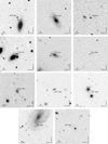 |
Fig. 1 The SNe in our sample and their environments. Short dashes mark the location of the respective supernova (see Table 1 for the exact coordinates). The images were taken in the SDSS i′ -band on MJD 56 520.89 for SN 2013eq, the i′ -band on MJD 56 462.90 for SN 2013ca, the r′ -band on MJD 56 625.03 for LSQ13cuw, the iPS1 -band on MJD 56 462.31 for PS1-13wr, the i′ -band on MJD 56 768.92 for PS1-14vk, the i′ -band on MJD 56 205.88 for PS1-12bku, the iPS1 -band on MJD 56 422.29 for PS1-13abg, the iPS1 -band on MJD 56 414.52 for PS1-13baf, the iPS1 -band on MJD 56 422.34 for PS1-13bmf, the iPS1 -band on MJD 56 422.29 for PS1-13atm, and the iPS1 -band on MJD 56 432.50 for PS1-13bni. |
The photometric coverage ranges from rather poor (with just one photometric epoch in gPS1 and rPS1 for PS1-13atm) to very good (e.g. for PS1-13baf, which has an average 5–8 day cadence coverage in gPS1rPS1iPS1zPS1 up to ~100 d after discovery). Most SNe show clear plateaus in their light curves identifying them as SNe II-P. The rPS1iPS1zPS1 decline rates of PS1-13bni have relatively large uncertainties, however they point towards a II-P classification.
A few SNe, namely LSQ13cuw, PS1-14vk and PS1-13baf, display decline rates after maximum that are higher than 0.5 mag/50 d, which – following the definition by Li et al. (2011) – places them in the SN II-L class. PS1-13atm shows only a very weak Hα absorption component, which is a SN II-L characteristic (see Gutiérrez et al. 2014). Furthermore the iPS1-band photometry is suggestive of a relatively long rise time ( ~>15 d), which could also be an indication that PS1-13atm is a Type II-L SN.
We are able to constrain the explosion epoch for LSQ13cuw, PS1-12bku, PS1-13abg, PS1-13baf, PS1-13bmf and PS1-13atm to a precision ranging from ± 0.1 d to ± 5.0 d using only photometric data, i.e. via pre-discovery non-detections, or a low-order polynomial fit to the rise time photometry.
All our SNe display the typical lines of Hα and Hβ in their spectra. Features stemming from weak lines of iron, in particular Fe iiλ5169 are visible in at least one spectrum for most, albeit not all, SNe.
Redshifts are derived either from the host galaxy or directly from the SN spectra. The redshifts are summarized in Table 1, while details of the redshift determination for the individual objects are presented in Appendix A.
The galactic extinction was adopted from the NASA/IPAC Extragalactic Database and is based on the values published by Schlafly & Finkbeiner (2011). A measure of the dust extinction within the SN host galaxy was obtainable only for selected SNe. For SN 2013eq a value of  = 0.062 ± 0.028 was adopted from Gall et al. (2016). Weak Na i D absorptions, are visible in the PS1-13wr spectra, which we use to determine the host galaxy extinction:
  .110 ± 0.049 (applying Eq. (9) from Poznanski et al. 2012). In most other cases we derived an upper limit to the equivalent width of the Na i D absorption and the extinction within the host galaxy. This process is described in detail in Appendix A.2. For our three highest-z SNe PS1-13bmf, PS1-13atm and PS1-13bni, we are not able to obtain a meaningful upper limit for the EW of the Na i D blend, due to the poor signal-to-noise ratio of their spectra.
3 Results and discussion
The EPM has been applied to a variety of SNe II. Detailed discussions of the EPM as well as examples of applying this technique in practice can be found e.g. in Kirshner & Kwan (1974), Schmidt et al. (1994a), Hamuy et al. (2001), Leonard et al. (2002a), Dessart & Hillier (2005), or Jones et al. (2009). We will closely follow the approach presented in Gall et al. (2016). We will use the dilution factors for the filter combination {BV I} as presented by Hamuy et al. (2001) and Dessart & Hillier (2005), respectively.
The SCM has been developed in Hamuy & Pinto (2002), Nugent et al. (2006), Poznanski et al. (2009), and D’Andrea et al. (2010). We follow the approach of Nugent et al. (2006), who modified the technique to be applicable for SNe at cosmologically significant redshifts.
In the following, we give a short overview of the use of SNe II-L as distance indicators up to this point (see Sect. 3.1) and then present the preparatory steps required to apply either the EPM or the SCM. These are the application of K-corrections (Sect. 3.2) and the determination of the temperatures (Sect. 3.3) and expansion velocities (Sect. 3.4). In particular, we will explore the possibility of using the Hα- or Hβ-velocities to estimate the photospheric velocity of Type II-P SNe (see Sect. 3.4.2). We then apply the EPM (Sect. 3.5) and SCM (Sect. 3.6) to our sample and compare the results in Sect. 3.7. Finally we create an EPM and a SCM Hubble diagram (Sect. 3.8) and investigate the implications of applying the EPM and SCM also to Type II-L SNe (Sect. 3.9).
3.1 Type II-L SNe as distance indicators
The Type II-L SN 1979C was used by Eastman et al. (1996) to derive an EPM distance of 15 ± 4 Mpc, which is consistent with the Cepheid distance of its host galaxy, NGC 4321 ( ~17 Mpc, e.g. Freedman et al. 1994). Another case is the Type II-L SN 1990K which was included in the SCM sample of Hamuy & Pinto (2002). Some SNe in the intermediate redshift SCM sample of Nugent et al. (2006) appear to have relatively steeply declining light curves (see e.g. SNLS-03D4cw in their Fig. 7 or SNLS-04D1ln in their Fig. 8).
Poznanski et al. (2009) select only objects with the lowest decline rates – i.e. Type II-P SNe – for their SCM sample, claiming that this reduces the scatter in the Hubble diagram. However, they also admit that only some of the steeper declining SNe II defy the velocity-luminosity correlation, while others do appear to be as close to the Hubble line as the rest of their sample. This was noted also by D’Andrea et al. (2010), who find that “none of the five most deviant SNe in [their] sample would be removed using the decline rate method”.
From a physical point of view we expect no fundamental difference between the progenitors of SNe II-P and II-L, i.e. we assume a one-parameter continuum depending mainly on the mass of the hydrogen envelope of the progenitor star at the time of explosion. This is corroborated by the work of Pejcha & Prieto (2015), who find that the main parameter determining the light curve shape is the photospheric temperature. Of course, other factors (such as metallicity) may influence the details of the explosion and its observational characteristics, thereby affecting the precision of distance measurements.
As was done by Rodríguez et al. (2014) and de Jaeger et al. (2017b), we include SNe with relatively fast decline rates in what follows, but we will discuss their application to distance measurements separately where appropriate.
3.2 K-corrections
In order to correctly apply the EPM in combination with the {BV I} dilution factors the photometry needs to be converted to the Johnson-Cousins filter system. EPM and SCM require the photometry to be transformed into the rest frame of each SN (see Eq. (13) in Gall et al. 2016).
We perform the transformations from the observed photometry to the rest frame Johnson-Cousins BV I filters in one step by calculating K-corrections with the SuperNova Algorithm for K-correction Evaluation (SNAKE) code within the S3 package (Inserra et al. 2018).
SNe with z < 0.13: the spectral coverage is sufficient to estimate valid K-corrections.
SNe PS1-13baf, PS1-13bmf and PS1-13atm: due to their redshifts above z ~ 0.14 the spectra of these SNe only partly cover the rest frame I-band. For this reason we combined the spectra of these three SNe with spectra from SNe 2013eq and 2013ca at similar epochs to obtain more accurate estimates for the respective K-corrections.
The K-corrections for PS1-13bni ( ) to the rest frame B- and V -band are determined using the available spectroscopy. The rest frame I-band K-corrections for PS1-13bni are calculated by interpolating the K-corrections from SNe 2013eq and 2013ca spectra to the epochs of the PS1-13bni spectra. This should provide valid results considering that most SNe II-P/L are relatively homogeneous in their spectral evolution. A small additional error in the I-band K-corrections for PS1-13bni cannot be excluded due to the unknown explosion times and the exact relative epochs of either SNe 2013eq, 2013ca and PS1-13bni.
3.3 Temperature evolution
In preparation for a temperature determination, the uncorrected observed photometry is interpolated to the epochs of spectroscopic observations, dereddened and K-corrected. For PS1-12bku, where photometry from multiple sources is available we first interpolate the K-corrections for each instrument to the epochs of photometric observations and then correct the photometry for dust extinction. The dereddened and K-corrected B, V , and I-band light curves are then interpolated to the epochs of spectroscopic observations.
Finally, the rest frame BVI magnitudes are converted into physical fluxes. The temperature at each epoch is estimated via a blackbody fit to the BVI-fluxes. To estimate the temperature uncertainties we performed additional blackbody fits spanning the extrema of the measured SN fluxes. The standard deviation of the resulting array of temperatures was taken as a conservative estimate of the temperature’s uncertainty.
The results are presented in Table B.1.
3.4 Velocities
3.4.1 Fe II λ5169
The EPM and the SCM require an estimate of the photospheric velocities. It has been argued that the Fe ii λ5169 absorption minimum provides a reasonable estimate of the photospheric velocity (Dessart & Hillier 2005). While the use of other weak lines, such as Fe ii λ5018, or Fe ii λλ4629, 4670, 5276, 5318 has also been discussed (e.g. Leonard et al. 2002a; Leonard 2002), here we will advance using the Fe ii λ5169 velocities when available. The relatively low quality of the spectra for the more distant SNe renders the measurement of weak lines impossible. For this same reason we also explore the possibility to estimate the Fe ii λ5169 velocity via the Hα or Hβ velocities.
3.4.2 Using Hα and Hβ to estimate photospheric velocities
Nugent et al. (2006) explored the ratio between the Hβ and the Fe iiλ5169 velocities and found a correlation. Poznanski et al. (2010) later improved this correlation and found that the Fe ii λ5169 velocities stand in a linear relation with the Hβ velocities5 : vH β /vFe 5169 = 1.19 . They included spectra from epochs between 5 and 40 days post-explosion. Our analysis is comparable to similar studies performed by Takáts et al. (2014); Rodríguez et al. (2014); de Jaeger et al. (2017b).
In order to test this relation we collected five well observed Type II-P SNe from the literature: SN 1999em (Leonard et al. 2002a; Leonard 2002), SN 1999gi (Leonard et al. 2002b), SN 2004et (Sahu et al. 2006), SN 2005cs (Pastorello et al. 2006, 2009), and SN 2006bp (Quimby et al. 2007). These objects were carefully selected on the basis of the quality and cadence of the available spectroscopy as well as for the good constraints on the explosion epochs. Note that none of the objects is of Type II-L, which might potentially exhibit different velocity evolutions than SNe II-P. A more detailed discussion follows in Sect. 3.4.3.
We determined Hβ and Fe ii λ5169 velocities up to ~70 d post explosion using iraf by fitting a Gaussian function to the minima of the respective lines and assumed an uncertainty of 5% for all velocity measurements. Takáts & Vinkó (2012) provided a detailed comparison of different measurement techniques for expansion velocities. The absorption method employed here was found to be equivalent to cross-correlation methods. In particular, they found that the Fe ii λ5169tends to underestimate the photospheric velocity at phases less than 40 days, while Hβ consistently overestimates the photospheric velocity. They further showed significant divergence of the Hβ velocities from the models at phases larger than 40 days. We determined exponential fits to the velocity evolution using:
 (1)
(1)
Here v(t⋆) is the velocity of a particular line at time t⋆ since explosion (rest frame)6 and a, b, and c are fit parameters. The uncertainty of each fit was estimated by calculating the root mean square of the deviation between the data and the fit. The explosion times for the five SNe were assumed to be as given in Gall et al. (2015, and references therein). The fit parameters are given in Table B.2.
In Fig. 2 we show the resulting relation between the Hβ and Fe ii λ5169 velocities in comparison with the corresponding relation as given by Nugent et al. (2006) and Poznanski et al. (2010) (areas shaded in green and yellow). The coloured points mark velocities measured between 5 and 40 days after explosion, while the gray points depict velocities measured either before day 5 or after day 40. While the relations from Nugent et al. (2006) and Poznanski et al. (2010) follow the general trend of the data, it is also clear that in particular at later epochs the velocities of the individual SNe evolve “away” from the linear relations. The fitted velocity evolution for each SN – depicted as solid lines in Fig. 2 – is not linear (as the Poznanski et al. 2010, relation) but rather acurve, only part of which lies in the linear regime.
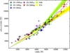 |
Fig. 2 Comparison of Hβ and Fe ii λ5169 velocities. The coloured points correspond to velocities measured between 5 and 40 days from explosion, while the gray points represent epochs either within 5 days of the explosion or after 40 days. The solid lines correspond to the fitted evolution of the Hβ and Fe ii λ5169 velocities for each SN. The green and yellow shaded regions reflect the vH β /vFe 5169 ratios as presented by Nugent et al. (2006) and Poznanski et al. (2010). |
We take a slightly different approach than Nugent et al. (2006) or Poznanski et al. (2010) in that we investigate the ratio between the Hβ and the Fe ii λ5169 velocities not as a function of velocity but rather as a function of time (i.e. epoch since explosion). At the same time, we also explore the viability of a relation between the Hα and the Fe ii λ5169 velocities, which might be a potential asset when dealing with spectra from high-z SNe II (such as those that will be routinely discovered by the LSST7 ) in which neither Fe ii λ5169 nor Hβ can be detected.
We interpolated the Hα, Hβ and Fe ii λ5169 velocities to all epochs up to ~70 days after explosion and then calculated the vH α /vFe 5169 and vH β /vFe 5169 ratios for each epoch and each SN, respectively (Fig. 3). The uncertainties of the individual line fits were propagated to estimate the uncertainty of the ratios. We then averaged the vH α /vFe 5169 and vH β /vFe 5169 ratios of the five SNe for each epoch (represented as black points in Fig. 3). The uncertainties were estimated by adding the uncertainties of the individual SN line ratios and the standard deviation of the five values at each epoch in quadrature. The latter is the dominant contributor to the uncertainty, indicating that the velocity evolution is distinct for each SN. The results are presented in Fig. 3 and listed in Table 2 for the vH α /vFe 5169 ratio and Table 3 for the vH β /vFe 5169 ratio.
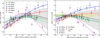 |
Fig. 3 vHα/vFe 5169 ratio (left panel) and vHβ/vFe 5169 ratio (right panel) compared to the rest frame epoch (from explosion). The thick dotted lines represent the vH α /vFe 5169 and vH β/vFe 5169 ratios for the individual SNe as well as the averaged ratios. For reasons of better visibility the uncertainty is depicted only for the averaged ratios and not for the fitted velocity ratios of the individual SN. Thecircle markers represent the measured vH α /vFe 5169 and vH β/vFe 5169 ratios for those epochs and SNe where spectroscopic data was available and both Hα (or Hβ) and the Fe ii λ5169 velocity could be measured. The yellow shaded band in the right panel corresponds to the ratio of vH β /vFe 5169 = 1.19 |

vHα/vFe 5169 ratio.
vHβ/vFe 5169 ratio.
At early epochs the individual vH α /vFe 5169 or vH β /vFe 5169 ratios of the five SNe scatter less than 10%. After about 40 days for Hα and about 30 days for Hβ the velocity ratios to Fe iiλ5169 of the various SNe begin to diverge significantly. A possible explanation is that during the cooling phase of the SN after the shock breakout, Type II-P SNe display relatively homogeneous properties: the hydrogen envelope is still fully ionized and the ejecta are expanding and cooling. Hydrogen recombination sets in only aftera few weeks and differences between the individual SNe in progenitor size, composition, or hydrogen envelope mass become apparent. This is reflected in the variety of luminosities and velocities observed for SNe II-P/L – in fact the relation between luminosity and velocity builds the basis for the standardized candle method (Hamuy & Pinto 2002). These differences are reflected also in the vH α /vFe 5169 or vH β /vFe 5169 ratios. A related pattern seems to be that the most extreme SNe in terms of deviation from the average ratios, SNe 2004et and 2005cs, display a relatively high ( ~ −17.2 mag for SN 2004et) or rather low ( ~ −15.1 mag for SN 2005cs) R/r-band maximum luminosity compared to the other objects (ranging between − 16.5 and − 16.9 mag).
The vH β /vFe 5169 ratio is flatter than the vH α /vFe 5169 ratio, suggesting that it depends less on epoch. The vH β /vFe 5169 ratio as constant within the errors between 5 and 30 days after explosion, which is in agreement with the results from Poznanski et al. (2010, shown in yellow in the right panel of Fig. 3). This result is also consistent with the findings of Takáts & Vinkó (2012) for early phases, where a nearly constant ratio of vH β /vFe 5169 can be inferred. The vH α /vFe 5169 ratio displays a stronger evolution with time.
3.4.3 Velocities in Type II-L SNe
The vH α -vFe 5169 and vH β -vFe 5169 relations were derived using only Type II-P SNe. While we expect SNe II-L to display similar properties in their velocity evolution as SNe II-P, we caution that applying the relations also for SNe II-L might introduce some systematic biases, e.g. due to the fact that SNe II-L are generally believed to produce more energetic ejecta than SNe II-P. It is also unclear whether the vH α /vFe 5169 and vH β /vFe 5169 ratios of individual SNe II-L would diverge at the same epoch as for SNe II-P.
Additionally, SNe II-L typically show smaller absorption components in their Hα features compared to SNe II-P (Gutiérrez et al. 2014). The extreme LSQ13cuw shows this can make a velocity determination challenging (see Sect. 3.5.4).
3.5 EPM distances
To measure the EPM distances for the SNe in our sample we apply Eqs. (13) and (14) from Gall et al. (2016):
 (2)
(2)
and
 (3)
(3)
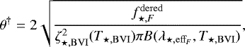
where  is the modified “angular size” of the SN,
  is the rest frame flux for the filter F, ζ⋆,BV I(T⋆,BV I) is the rest frame dilution factor for the filter combination {BV I} at the rest frame BVI-temperature T⋆,BV I,
  is the effective wavelength of the corresponding filter F, in the rest frame,
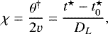
  is the black body function, v is the photospheric velocity, t⋆ the time after explosion at
  in the SN frame, and DL is the luminosity distance of the SN.
As in Gall et al. (2016) we use the temperature dependent {BVI} dilution factors presented by Hamuy et al. (2001, based on the dilution factors calculated by Eastman et al. 1996) and Dessart & Hillier (2005). The Fe iiλ5169 velocities were used for the distance determinations if measureable. For the SNe where the Fe iiλ5169 feature could not be securely identified, we applied the vHα/vFe 5169 and/or vHβ/vFe 5169 ratio, to estimate the photospheric velocities and the SN distance.
As pointed out by Schmidt et al. (1992) EPM suffers less from extinction than other methods. An error in the extinction correction will lead to a compensating effect between temperature and luminosity of the SN. These lead to a reduction of the influence of extinction on the distance determination through EPM.
The distances were calculated by determining χ for each filter (B, V , and I) and epoch. To estimate the uncertainties of both the distance DL and the time of explosion  , we performed additional fits to all combinations of adding or subtracting the uncertainties of χ. The standard deviation of the resulting arrays of distances and explosion times was taken as a conservative estimate of their respective uncertainties.
3.5.1 Commonalities
Figures 4 and 5 show the distance fits for PS1-14vk and are representative for the χ-t⋆-fits made for all SNe (see Figs. C.1–C.7). We use PS1-14vk as an example to outline a number of commonalities.
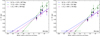 |
Fig. 4 Distance fits for PS1-14vk using all available epochs and ζBVI as givenin Hamuy et al. (2001; left panel) and Dessart & Hillier (2005; right panel). The diamond markers denote values of χ through which the fit is made. |
-
The results using either the dilution factors by Hamuy et al. (2001) or Dessart & Hillier (2005) are very similar for all SNe. The dilution factors by Dessart & Hillier (2005) systematically yield slightly larger distances.
-
The V -band distance is systematically smaller and the explosion epoch later than for the BI-bands. The exception of the rule is PS1-13baf, where the V -band distances are larger than derived from B- and I-band. Discrepancies in the EPM distances when using different filter combinations have previously been observed (e.g. Hamuy et al. 2001; Jones et al. 2009).
-
For some SNe the photometry provides an independent constraint on the time of explosion. In theses cases we use the “observed” explosion epoch as an additional data point in the fit and are able to significantly reduce the error in the distance determination.
-
The vH β /vFe 5169 ratio was applied only up to ~30 days from explosion.
-
Jones et al. (2009) argue that after around 40 days from explosion the linearity of the θ∕v versus t relation in Type II-P SNe deteriorates. Considering the scarcity of data points for our SNe, we use data up to ~60 days from explosion for the distance fits, whenever viable. The χ–t⋆ relation seems to be linear also in this extended regime see Appendix sectionlinking B.1 . For PS1-14vk, a Type II-L SN, we observe a breakdown in the linearity of the χ–t⋆ relation after 30 days after discovery cf. Fig. 5. Taking into account the epoch of explosion ~20 days before discovery, this corresponds to a breakdown in the linearity of the χ–t⋆ relation sometime between ~50 and ~70 days post explosion. When performing a χ–t⋆ fit beyond the linear regime the distances are overestimated significantly and the estimated epoch of explosion is considerably earlier than when using only the linear regime.
-
Our errors on the distances (averaged over the BV I filters) span a wide range between ~3% and ~54%, essentially depending on the quality of the available data for each SN. A strong constraint on the epoch of explosion reduces the uncertainty of the distance fit significantly. The errors account for the uncertainties from the photometry, the SN redshift, the K-corrections, the photospheric velocities and – for SNe 2013eq and PS1-13wr – the dust extinction in the host galaxy.
The velocities and dilution factors that were used to derive various values of θ† are presented in Table B.3, while our final distance results are summarized in Table 4. In the following we outline the particularities for each individual SN.
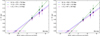 |
Fig. 5 Distance fits for PS1-14vk using only epochs that follow a linear relation and ζBVI as givenin Hamuy et al. (2001; left panel) and Dessart & Hillier (2005; right panel). The diamond markers denote values of χ through which the fit is made. |
EPM distances and explosion times for the SNe in our sample.
3.5.2 SN 2013eq
SN 2013eq is presented in detail in Gall et al. (2016). Using the dilution factors from Hamuy et al. (2001), Gall et al. (2016) found a luminosity distance of DL = 151 ± 18 Mpc and an explosion time of 4.1 ± 4.4 days before discovery (rest frame), corresponding to a  of MJD 56 499.6 ± 4.6 (observer frame). Applying the dilution factors from Dessart & Hillier (2005) DL = 164 ± 20 Mpc and an explosion time of 3.1 ± 4.1 days before discovery (rest frame) corresponding to a
  of MJD 56 500.7 ± 4.3 (observer frame) were measured.
3.5.3 SN 2013ca
Good quality spectroscopy is available for SN 2013ca allowing us to determine the photospheric velocity directly from the Fe ii λ5169 line. The photometric coverage is poor, with only 2 points observed in each of the LT g′ r′ i′ filters. The flux at the epochs of spectroscopic observations was linearly interpolated through those two data points. This should be a reasonable assumption for a Type II-P SN during the plateau phase.
3.5.4 LSQ13cuw (SN II-L)
LSQ13cuw photometry and spectroscopy was adopted from Gall et al. (2015). They constrain the epoch of explosion to MJD 56 593.4 ± 0.7. This was used as a further data point in the distance fit and provides a more accurate result. Unfortunately, lines of Fe ii λ5169 are not visible in any of the LSQ13cuw spectra and we applied the vH β /vFe 5169 ratio to estimate the photospheric velocities.
However, the spectra of LSQ13cuw are characterised by Hα and Hβ features that show almost no absorption component, which makes a velocity determination difficult. We were only able to confidently measure the Hβ velocity after +32 days. However, as outlined in Sect. 3.4.2 the vH β − vFe 5169 relation is not reliable after ~30 days from explosion. This leaves us with only one estimate for the photospheric velocity from the +32 d spectrum.
3.5.5 PS1-13wr
The reasonably high signal-to-noise spectra of PS1-13wr allow us to determine the photospheric velocity directly from the Fe iiλ5169 line. The errors in the distance determination of PS1-13wr are larger than for other SNe due to the uncertainty of the dust extinction within the host galaxy (Table 1).
3.5.6 PS1-14vk (SN II-L)
The photospheric velocity of PS1-14vk was measured from the Fe iiλ5169 line for all epochs, except ~2 d and ~14 d post-discovery, where the line was either not visible or blended.
The values of χ in PS1-14vk for the epochs +11, +27, and +33 d follow a clearly linear relation in contrast to the last epoch at +49 d after discovery (see discussion in Sect. 3.5.1). This is independent whether we apply the dilution factors given by Hamuy et al. (2001) or Dessart & Hillier (2005). Consequently, we performed fits only through χ values at +11, +27, and +33 days.
3.5.7 PS1-12bku
The Fe iiλ5169 line in the PS1-12bku spectra was used to estimate the photospheric velocity. We can additionally constrain the fits by using the estimate for the explosion epoch available for PS1-12bku. This reduces the distance uncertainties significantly.
3.5.8 PS1-13abg
Only poor quality spectra are available for PS1-13abg and we can identify the Fe ii λ5169 line only in the +44 d spectrum. We use this measurement and the loose constraint for the explosion epoch to estimate the distance to PS1-13abg.
3.5.9 PS1-13baf
The spectraof PS1-13baf have a poor signal-to-noise ratio and we are not able to identify Fe ii λ5169 line in any of the spectra. We apply the vH β /vFe 5169 relation to the first two epochs (i.e. before ~30 days), to estimate the photospheric velocities. The estimate for the explosion epoch reduces the error in the distance.
3.5.10 PS1-13bmf (SN II-L)
The spectra of PS1-13bmf at the first two epochs (+5 d and +8 d) are basically featureless. The Fe ii λ5169 line could be identified at +29 and +47 days. We additionally constrain the fits by using the estimate for the explosion epoch available for PS1-13bmf (Appendix A.9).
3.5.11 PS1-13atm (SN II-L)
The photometric coverage of PS1-13atm, our second-highest redshift SN, is insufficient to perform reliable fits for an estimate of the BV I magnitudes at the epochs of spectroscopic observations. The gPS1 - and rPS1 -band have only a single data point each. We therefore forgo an attempt to calculate an EPM distance to PS1-13atm.
3.5.12 PS1-13bni
The Fe ii λ5169 line could not be clearly identified at any epoch of PS1-13bni. We relied entirely on estimates of the photospheric velocities using the Hβ line (at +15 and +24 days) and the vHβ/vFe 5169 relation. We note that the relation is prone to large uncertainties at epochs ≳50 days post explosion.
Since the vHβ/vFe 5169 relation is epoch dependent, but no estimate of an explosion epoch from other sources is available for PS1-13bni, we pursue an iterative approach to derive the time of explosion. For the initial iteration we assume the first detection to be the time of explosion and evaluate the vHβ/vFe 5169 relation at the resulting epochs. Then we fit for the distance and the explosion epoch as would be done for any other SN. The derived explosion epoch is then used as a base for the second iteration, and the spectral epochs as well as vHβ/vFe 5169 ratios are adjusted accordingly. We repeat this process until the explosion time converges.
3.6 SCM distances
The V - and I-band corrected photometry was also used for SCM. The light curves are interpolated to 50 days after explosion.
The expansion velocity is determined using the relation published by Nugent et al. (2006, Eq. (2)):
 (4)
(4)
where v(t⋆) is the Fe iiλ5169 velocity at time t⋆ after explosion (rest frame). For the SNe where we could not identify the Fe iiλ5169 feature in their spectra we first applied the vHβ/vFe 5169 relation and then utilized the derived Fe iiλ5169 velocities to estimate the expansion velocity at day 50. This procedure was carried out twice for those SNe where estimates of the explosion epoch where available via the EPM (depending on dilution factors).
Finally, we use Eq. (1) in Nugent et al. (2006) to derive the distance modulus:
![Mathematical equation: $ M_{I_{50}} = -\alpha\, \mathrm{log}_{10}\left(\frac{ v_{50,\mathrm{Fe\,{{II}}}} }{5000}\right) - 1.36 \left[ (V - I)_{50} - (V - I)_0 \right] + M_{I_0} , $](/articles/aa/full_html/2018/03/aa31271-17/aa31271-17-eq30.png) (5)
(5)
where MI is the rest frame I-band magnitude, (V − I) the colour, and v is the expansion velocity each evaluated at 50 days after explosion. The parameters are set as follows: α = 5.81,  (for an H0 of 70 km s−1 Mpc−1) and
  , following Nugent et al. (2006).
Our results are shown in Table 5. Additionally, we adopt the SCM distances derived by Gall et al. (2016) for SN 203eq: DL = 160± 32 Mpc and DL = 157± 31 Mpc, using the explosion epochs calculated via the EPM and utilizing the dilution factors either from Hamuy et al. (2001) or Dessart & Hillier (2005).
SCM quantities and distances.
The final errors on individual distances span a range between 11 and 35% depending mainly on whether the explosion epoch is well constrained or not. The I-band magnitude and the (V − I) colour will not change significantly during the plateau phase of Type II-P SNe and are therefore relatively robust; however, this is not true for the expansion velocity. Any uncertainty in the explosion epoch directly translates into an uncertainty in the 50 d velocity and thereby affects the precision of the distance measurement. In our sample this is borne out in the fact that the SCM distances derived using estimates for the explosion epoch from photometry, have significantly smaller relative uncertainties, than those derived using estimates via the EPM.
3.7 Comparison of EPM and SCM distances
Figure 6 compares the EPM and SCM distances for the entire sample. There appears no obvious trend for one technique to systematically result in longer or shorter distances; a shift would indicate H0 ≠ 70 km s−1 Mpc−1. No obvious systematic shift can be discerned amongst the SNe using the Fe ii λ5169 line for the EPM and SCM distances as an estimator for the photospheric velocity.
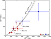 |
Fig. 6 Comparison of EPM and SCM distances, using the dilution factors by Dessart & Hillier (2005). Filled circles denote SNe with the explosion epoch obtained via EPM, while stars mark SNe with the explosion epoch estimated from pre-discovery photometry. The three Type II-L SNe are labelled specifically. Different colours denote the line that was used to estimate the photospheric velocities: red corresponds to Fe ii λ5169, and dark blue to Hβ. The solid line shows the |

3.8 The Hubble diagram
Figure 7 shows the Hubble diagrams using EPM (left panel) and SCM distances (right panel), respectively. The red and blue points represent SNe from our sample for which either Fe ii λ5169 or Hβ was used to estimate the photospheric velocities. For reasons of better visibility we only depict our distance results using the Dessart & Hillier (2005) dilution factors, which give somewhat larger distances than the Hamuy et al. (2001) dilution factors. Our conclusions are the same regardless of which set of dilution factors is used. The grey points depict SNe from other samples. The solid line in both panels represents a ΛCDM cosmology (H0 = 70 km s−1 Mpc−1, Ωm = 0.3 and ΩΛ = 0.7.8 ). The three Type II-L SNe LSQ13cuw, PS1-14vk and PS1-13bmf are labelled in both the EPM and the SCM Hubble diagrams.
3.8.1 EPM Hubble diagram
Our EPM measurements are complemented by EPM distances from the samples of Eastman et al. (1996, Table 6), Jones et al. (2009, Table 5) and Bose & Kumar (2014, Table 3) in the EPM Hubble diagram (left panel of Fig. 7). In the cases of Jones et al. (2009) and Bose & Kumar (2014) we selected the distances given using the Dessart & Hillier (2005) dilution factors. In addition, Bose & Kumar (2014) give alternate results for the SNe 2004et, 2005cs, and 2012aw, for which constraints for the explosion epoch are available. We chose those values rather than the less constrained distance measurements. Note that SN 1992ba appears in Jones et al. (2009) and Eastman et al. (1996), while SN 1999gi was published in Jones et al. (2009) and Bose & Kumar (2014).
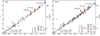 |
Fig. 7 SN II Hubble diagrams using the distances determined via EPM (left panel) and SCM (right panel). EPM Hubble diagram (left): the distances derived for our sample (circles) use the dilution factors from Dessart & Hillier (2005). The different colours denote the absorption line that was used to estimate the photospheric velocities (Fe ii λ5169 – red; Hβ – blue). We also included EPM measurements from Eastman et al. (1996, E96), Jones et al. (2009, J09) and Bose & Kumar (2014, B14). The solid line corresponds to a ΛCDM cosmology with H0 = 70 km s−1 Mpc−1, Ωm = 0.3 and ΩΛ= 0.7, and the dotted lines to the range covered by an uncertainty on H0 of 5 km s−1 Mpc−1. SCM Hubble diagram (right): circle markers depict the SCM distances derived for our sample using the explosion epochs previously derived via EPM and the dilution factors from Dessart & Hillier (2005). The star shaped markers depict SNe for which an independent estimate of the explosion time was available via photometry. The colours are coded in the same way as for the EPM Hubble diagram. Similarly, the solid and dotted lines portray the same relation between redshift and distance modulus as in the left panel. We also included SCM distances from Poznanski et al. (2009, P09), Olivares et al. (2010, O10) and D’Andrea et al. (2010, A10). We separated the objects “culled” by Poznanski et al. (2009) from the rest of the sample by using a different symbol. The three Type II-L SNe LSQ13cuw, PS1-14vk and PS1-13bmf are identified in both the EPM and the SCM Hubble diagram. |
The SN distances trace the slope of the Hubble line within the uncertainties. This is an indication that the relative distances are measured to a rather high accuracy.
3.8.2 SCM Hubble diagram
The SCM Hubble diagram shows our sample alongside SCM distances from Poznanski et al. (2009, Table 2), Olivares et al. (2010, Table 8) and D’Andrea et al. (2010, Table 3). The Poznanski et al. (2009) sample contains all objects from Nugent et al. (2006). We also included those objects that Poznanski et al. (2009) rejected due to their higher decline rates. D’Andrea et al. (2010) do not give the distance measurements directly but rather their derived values for the I-band magnitude, the (V − I)-colour and the velocity 50 days after explosion (rest frame). We used these to apply the same equation and parameters from Nugent et al. (2006) as for our own sample, to find the distances to these objects. Note that the Poznanski et al. (2009) and Olivares et al. (2010) have a number of SNe in common : SNe 1991al, 1992af, 1992ba, 1999br, 1999cr, 1999em, 1999gi, 2003hl, 2003iq, and 2004et.
Our SCM distances scatter around the H0 = 70 km s−1 Mpc−1 as SCM is based on a previously chosen value of H0 (following Nugent et al. 2006).
There seems to be no obvious difference in the scatter for SNe with an estimate of the explosion epoch based on SN photometry or those relying on an EPM estimate for the time of explosion. This implies either that the epochs of explosion derived via the EPM are fairly accurate, or that constraints on the explosion epoch of only a few days, are not relevant for precise SCM measurements.
3.8.3 PS1-13bni
Finally, we would like to point out that our distance measurements to PS1-13bni (at a redshift of  ) demonstrates that both the EPM and the SCM bear great potential for cosmology. This statement is, however, tainted by the large uncertainties in the decline rates of PS1-13bni, and the implication that PS1-13bni could be a Type II-L SN and the open question whether these can be used as distance indicators.
3.9 Applying the EPM and SCM to Type II-L SNe
When considering the use of SNe II-L for cosmology a few peculiarities must be considered. As discussed in Sect. 3.4.3 it is unclear whether SNe II-L display the same velocity evolution as SNe II-P and whether the vHα/vFe 5169 and vHβ/vFe 5169 ratios evolve similarly for SNe II-L and SNe II-P. Pejcha & Prieto (2015) find a physical answer to this question by showing that the light curve shape is mostly determined by temperature changes in the photosphere. For EPM with SNe II-L the additional question arises whether the relation between χ and t⋆ is linear for SNe II-L (see Eq. (3)). The case of PS1-14vk indicates that this linear relation might be valid for a similar period of time as for SNe II-P (see Sect. 3.5.1).
Although SNe II-L fade faster than SNe II-P, they are on average brighter. Gall et al. (2015) suggest that SNe II-L might have slightly longer rise times than SNe II-P. This somewhat facilitates obtaining pre-maximum data, resulting in a better constraint on the explosion epoch. The uncertainty in the explosion epoch contributes significantly to the total error budget (cf. also Pejcha & Prieto 2015).
The three Type II-L SNe LSQ13cuw, PS1-14vk, and PS1-13bmf, are indistinguishable from the rest of the sample, in the EPM and the SCM Hubble diagrams. We find once again (cf. Sect. 1) that there is no clear observational distinction between the SNe II-P and II-L classes nor is one expected on theoretical grounds. Testing the validity of Type II-P SN relations, like the χ–t⋆ relation in the EPM, or the velocity–luminosity correlation for the SCM for SNe with a range of decline rates, will help to better understand the sources of systematic uncertainties for both techniques.
4 Conclusions
Optical light curves and spectra of nine Type II-P/L SNe with redshifts between z = 0.045 and z = 0.335: SN 2013ca, PS1-13wr, PS1-14vk, PS1-12bku, PS1-13abg, PS1-13baf, PS1-13bmf, PS1-13atm and PS1-13bni were presented. To this sample, we added the Type II-P SN 2013eq (Gall et al. 2016, z = 0.041± 0.001) and the Type II-L SN LSQ13cuw (Gall et al. 2015, z = 0.045 ± 0.003) to derive distances utilizing the expanding photosphere method and the standardized candle method. The procedures presented in Gall et al. (2016) for EPM at cosmologically significant redshifts and the approach of Nugent et al. (2006) for the SCM were adopted.
The possibility of estimating the photospheric velocities in Type II-P/L SNe Hα and Hβ was explored. We used five well observed SNe (SNe 1999gi, 1999em, 2004et, 2005cs, and 2006bp) to calculate anepoch-dependent relation between the Hα and Hβ velocities relative to the Fe ii λ5169 velocity. The vH α /vFe 5169 and vH β /vFe 5169 ratios are in good agreement at early epochs ( ≤40 days after explosion) for Hα and ≤30 days for Hβ. The scatter in these velocity ratios is between 4 and 14%. At later epochs the vH α /vFe 5169 and vH β /vFe 5169 ratios diverge significantly between individual SNe.
For the utilization in the EPM and the SCM we used the Fe ii λ5169 line as an estimator of the photospheric velocity where ever possible. In cases where no Fe ii λ5169 feature could be identified we applied the vH β /vFe 5169 relation to obtain an estimate for the velocity.
Our EPM and SCM distances are in good agreement with the expectations from standard ΛCDM cosmology. This is especially encouraging given the varied quality of the available data for local versus intermediate- or high-redshift objects. Comparable precision to other distance indicators can feasibly be achieved via larger samples and higher quality data of Type II SNe.
The case of PS1-13bni at a spectroscopically derived redshift of  is the highest-z SN II for which a distance measurement was ever attempted, further demonstrating the potential of the EPM and SCM for cosmological applications.
Finally, we evaluated the implications of using Type II-L SNe for cosmology. Our sample contains three Type II-L SNe that yield similar distances compared to the SNe II-P. Including SNe II-L would allow for larger samples to be considered. However, we note that that future investigations on the differences and similarities between SNe II-L and II-P are necessary to robustly assess any systematics. Although currently only demonstrated for local SNe (Maguire et al. 2010), further improvements may also be possible by incorporating infrared datasets for SNe within the Hubble flow.
Acknowledgements
Based in part on observations made with the Gran Telescopio Canarias (GTC2007-12ESO, ESO program ID: 189.D-2007, PI:RK), installed in the Spanish Observatorio del Roque de los Muchachos of the Instituto de Astrof?sica de Canarias, on the island of La Palma. E.E.E.G., B.L., S.T., and W.H. acknowledge partial support by the Deutsche Forschungsgemeinschaft through the TransRegio project TRR33 “The Dark Universe”. R.K. acknowledges funding from STFC (ST/L000709/1). N.M. acknowledges support from the Science and Technology Facilities Council [ST/L00075X/1]. Based in part on observations obtained at the Liverpool Telescope (program ID: XIL10B01, PI:RK), operated on the island of La Palma by Liverpool John Moores University in the Spanish Observatorio del Roque de los Muchachos of the Instituto de Astrof?sica de Canarias with financial support from the UK Science and Technology Facilities Council. Based in part on observations obtained at the Nordic Optical Telescope, operated by the Nordic Optical Telescope Scientific Association at the Observatorio del Roque de los Muchachos, La Palma, Spain, of the Instituto de Astrof?sica de Canarias. This research has made use of the NASA/IPAC Extragalactic Database (NED) which is operated by the Jet Propulsion Laboratory, California Institute of Technology, under contract with the National Aeronautics and Space Administration. The Pan-STARRS1 Surveys (PS1) have been made possible through contributions of the Institute for Astronomy, the University of Hawaii, the Pan-STARRS Project Office, the Max-Planck Society and its participating institutes, the Max Planck Institute for Astronomy, Heidelberg and the Max Planck Institute for Extraterrestrial Physics, Garching, The Johns Hopkins University, Durham University, the University of Edinburgh, Queen’s University Belfast, the Harvard-Smithsonian Center for Astrophysics, the Las Cumbres Observatory Global Telescope Network Incorporated, the National Central University of Taiwan, the Space Telescope Science Institute, the National Aeronautics and Space Administration under Grant No. NNX08AR22G issued through the Planetary Science Division of the NASA Science Mission Directorate, the National Science Foundation under Grant No. AST-1238877, the University of Maryland, and Eotvos Lorand University (ELTE) and the Los Alamos National Laboratory. Funding for the Sloan Digital Sky Survey (SDSS) and SDSS-II has been provided by the Alfred P. Sloan Foundation, the Participating Institutions, the National Science Foundation, the U.S. Department of Energy, the National Aeronautics and Space Administration, the Japanese Monbukagakusho, the Max Planck Society, and the Higher Education Funding Council for England. The SDSS Web Site is http://www.sdss.org/. The SDSS is managed by the Astrophysical Research Consortium for the Participating Institutions. The Participating Institutions are the American Museum of Natural History, Astrophysical Institute Potsdam, University of Basel, University of Cambridge, Case Western Reserve University, University of Chicago, Drexel University, Fermilab, the Institute for Advanced Study, the Japan Participation Group, Johns Hopkins University, the Joint Institute for Nuclear Astrophysics, the Kavli Institute for Particle Astrophysics and Cosmology, the Korean Scientist Group, the Chinese Academy of Sciences (LAMOST), Los Alamos National Laboratory, the Max-Planck-Institute for Astronomy (MPIA), the Max-Planck-Institute for Astrophysics (MPA), New Mexico State University, Ohio State University, University of Pittsburgh, University of Portsmouth, Princeton University, the United States Naval Observatory, and the University of Washington.
Note added in proof. During the refereeing process de Jaeger et al. (2017a) was published. It reports the observations of a more distant Type II SN, SN 2016jhj at z = 0.34, although with a single spectrum and hence the application of the SCM only.
Appendix A Photometricand spectroscopic observations of the individual SNe
An overviewof the SN sample is given in Sect. 2, Table 1. In the following we present the data for each individual SN. All epochs are given in the SN rest frame.
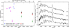 |
Fig. A.1 SN 2013ca. Left panel: LT g′ r′ i′ and LSQ V light curves of SN 2013ca. The vertical ticks on the top mark the epochs of the observed spectra. ATel 5056: Walker et al. (2013); CBET 3508: Zhang et al. (2013). Right panel: SN 2013ca spectroscopy. (*) Flux normalized to the maximum Hα flux for better visibility of the features. The exact normalizations are: flux/1.3 for the +30 d spectrum; flux/1.4 for +34 d; flux/1.5 for +46 d; flux/1.5 for +60 d. |
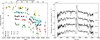 |
Fig. A.2 PS1-13wr. Left panel: grizyPS1 light curves of PS1-13wr. The vertical ticks on the top mark the epochs of the observed spectra. Right panel: PS1-13wr spectroscopy. (*) Flux normalized to the maximum Hα flux for better visibility of the features. The exact normalizations are: flux/3.4 for the +12 d spectrum; flux/3.5 for +18 d; flux/3.6 for +25 d; flux/3.6 for +41 d. |
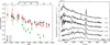 |
Fig. A.3 PS1-14vk. Left panel: LT g′ r′ i′ light curves of PS1-14vk. The vertical ticks on the top mark the epochs of the observed spectra. Right panel: PS1-14vk spectroscopy. (*) Flux normalized to the maximum Hα flux for better visibility of the features. The exact normalizations are: flux/2.6 for the +2 d spectrum; flux/2.7 for +11 d; flux/2.8 for +14 d; flux/2.3 for +27 d; flux/2.1 for +33 d; flux/1.9 for +49 d. |
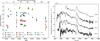 |
Fig. A.4 PS1-12bku. Left panel: grizyPS1 and NOT u′g′r′i′z′ light curves of PS1-12bku. The vertical ticks on the top mark the epochs of the observed spectra. Right panel: PS1-12bku spectroscopy. (*) Flux normalized to the maximum Hα flux for better visibility of the features. The exact normalizations are: flux/3.3 for the +23 d spectrum; flux/3.6 for +27 d; flux/3.5 for +41 d; flux/2.9 for +81 d. |
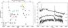 |
Fig. A.5 PS1-13abg. Left panel: grizyPS1 light curves of PS1-13abg. The vertical ticks on the top mark the epochs of the observed spectra. Right panel: PS1-13abg spectroscopy. (*) Flux normalized to the maximum Hα flux for better visibility of the features. The exact normalizations are: flux/0.7 for the +7 d spectrum; flux/0.8 for +32 d; flux/1.1 for +44 d. |
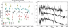 |
Fig. A.6 PS1-13baf. Left panel: grizyPS1 light curves of PS1-13baf. The vertical ticks on the top mark the epochs of the observed spectra. Right panel: PS1-13baf spectroscopy. (*) Flux normalized to the maximum Hα flux for better visibility of the features. The exact normalizations are: flux/4.1 for the +16 d spectrum; flux/3.2 for +28 d; flux/2.9 for +39 d. |
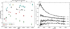 |
Fig. A.7 PS1-13bmf. Left panel: grizyPS1 light curves of PS1-13bmf. The vertical ticks on the top mark the epochs of the observed spectra. Right panel: PS1-13bmf spectroscopy. (*) Flux normalized to the maximum Hα flux for better visibility of the features. The exact normalizations are: flux/5.7 for the +5 d spectrum; flux/9.5 for +8 d; flux/8.8 for +29 d; flux/5.1 for +47 d. |
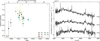 |
Fig. A.8 PS1-13atm. Left panel: grizyPS1 light curves of PS1-13atm. The vertical ticks on the top mark the epochs of the observed spectra. Right panel: PS1-13atm spectroscopy. (*) Flux normalized to the maximum Hα flux for better visibility of the features. The exact normalizations are: flux/4.3 for the +16 d spectrum; flux/6.1 for +23 d; flux/7.8 for +44 d. |
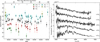 |
Fig. A.9 PS1-13bni. Left panel: grizyPS1 light curves of PS1-13bni. The vertical ticks on the top mark the epochs of the observed spectra. Right panel: PS1-13bni spectroscopy. (*) Flux normalized to the maximum Hα flux for better visibility of the features. The exact normalizations are: flux/2.5 for the +14 d spectrum; flux/2.5 for +15 d; flux/2.5 for +24 d; flux/2.2 for +32 d; flux/2.1 for +51 d. |
SN 2013ca: Photometric observations.
SN 2013ca: Journal of spectroscopic observations.
PS1-13wr: photometric observations.
PS1-13wr: Journal of spectroscopic observations.
A.1 SN 2013eq
Photometric data up to 76 days after discovery and a series of five spectra ranging from 7 to 65 days after discovery for SN 2013eq are presented in Gall et al. (2016). They find a redshift of z = 0.041 ± 0.001, a host galaxy extinction of  mag and a Galactic extinction of
  mag from Schlafly & Finkbeiner (2011). We adopt these values also for this study.
A.2 SN 2013ca
SN 2013ca was discovered on 2013 April 21 as “LSQ13aco” by the La Silla Quest Supernova Survey (LSQ; Baltay et al. 2013), and spectroscopically classified as a Type II-P SN (Walker et al. 2013). It was independently discovered on 2013 May 1 and likewise classified as a Type II-P SN by Zhang et al. (2013), who also report further detections on 2013 April 10 and May 3.
We obtained LT g′r′i′ photometry 41 and 68 days after the first detection and a series of four GTC spectra ranging between +30 and +60 days after the first detection.
In order to determine the redshift of SN 2013ca we extracted host galaxy spectra alongside the SN spectra and measured the redshift of the narrow Hα emission line. Averaging over all epochs results in z = 0.045 ± 0.001.
Features attributable to the Na i doublet from interstellar gaseither in the Milky Way or the host galaxy are not apparent in the spectra of SN 2013ca. In order to derive an upper limit to the equivalent width (EW) of a Na i D absorption, we constructed a weighted stack of all SN 2013ca spectra, where the weights reflect the signal-to-noise ratio. We then created a series of artificial Gaussian profiles centred at 5893 Å and subtracted these from the stacked spectrum. The FWHM of the Gaussian profiles was set to 17.0 Å, which corresponds to our lowest resolution spectrum. We increased the EW of the artificial profile in steps of 0.1 Å in order to determine the limiting EW at which an artificial line profile as described above would be detectable in the stacked spectrum. Using this method we derive an upper limit for the EW of the Na i D λλ 5890, 5896 blend to be <0.4 Å. Applying the relation in Eq. (9) of Poznanski et al. (2012), we find  mag.
mag.
The light curves of SN 2013eq are presented in the left panel of Fig. A.1. Table A.1 shows the log of photometry and the calibrated magnitudes. The photometric coverage of SN 2013ca is sparse. The two available data points in r′ yield a decline rate of 0.34 ± 0.18 mag/50 d, which is below the threshold of 0.5 mag/50 d set by Li et al. (2011) to distinguish SNe II-P from SNe II-L.
Table A.2 gives the journal of spectroscopic observations. The calibrated spectra of SN 2013ca are presented inthe right panel of Fig. A.1. They are corrected for galactic reddening and redshift (z = 0.045). The Hα line shows only a small absorption at +30 and +34 days, which becomes more prominent at +46 d and +60 days. Weak Fe ii λ5169 is visible at all four epochs.
A.3 LSQ13cuw
Photometricdata up to 100 days after discovery and 5 spectra ranging between 25 and 84 days after discovery for LSQ13cuw were presented by Gall et al. (2015). Performing a fit to the pre-peak photometry Gall et al. (2015) are able to constrain the epoch of explosion to be MJD 56 593.42 ± 0.68. They find a redshift of z = 0.045 ± 0.003, a host galaxy extinction  < 0.16 mag and a Galactic extinction of
  = 0.023 mag from Schlafly & Finkbeiner (2011). We adopt these values here.
A.4 PS1-13wr
PS1-13wr was discovered on 2013 February 26 by the PS1 MD survey. gPS1 rPS1iPS1zPS1yPS1 photometry was obtained in the course of the PS1 MD survey up to 150 days after the first detection. We obtained 4 GTC spectra ranging from +12 to +41 days after discovery.
PS1-13wr lies close to the galaxy SDSS J141558.95+520302.9 for which the SDSS reports a spectroscopic redshift of 0.076 ± 0.001. This redshift was adopted also for PS1-13wr and is consistent with the redshift of the Na i D doublet visible in the spectra of PS1-13wr.
In order to obtain an accurate measure of the Na i D equivalent width we constructed a weighted stack of all PS1-13wr spectra, where the weights reflect the signal-to-noise ratio in the 5850–6000 Å region. We measure an equivalent width of EW Na I D = 0.76 ± 0.07 Å in the stacked PS1-13wr spectrum. Applying the empirical relation between Na i D absorption and dust extinction given in Poznanski et al. (2012, Eq. (9)), this translates into an extinction within the host galaxy of  mag.
mag.
The light curves of PS1-13wr are presented in the left panel of Fig. A.2. Table A.3 gives the log of imaging observations and the calibrated magnitudes. PS1-13wr displays a distinct plateau in the rPS1 -, iPS1 -, zPS1 -, and yPS1 -bands until about 80 days after discovery, when it drops onto the radioactive tail. The rPS1 -band decline rate is ~0.20 ± 0.07 mag/50 days characterising it as a II-P SN.
Table A.4 lists the journal of spectroscopic observations for PS1-13wr. The calibrated spectra of PS1-13wr are presented in the right panel of Fig. A.2. They are corrected for galactic and host galaxy reddening as well as redshift (z = 0.076). The spectra display the typical features of Hα and Hβ. The Hα lines in all four spectra have a clear P-Cygni profile shape. It additionally displays a narrow emission component which is likely a contamination from the host galaxy. Weak lines of iron, in particular Fe iiλ5169 are visible in all four spectra.
A.5 PS1-14vk
PS1-14vk was discovered on 2014 March 24 by the PS1 3π survey. We obtained LT g′r′i′ photometry up to 68 days after discovery and 6 GTC spectra ranging from +2 to +49 days after first detection.
PS1-14vk lies in the vicinity of the galaxy SDSS J121045.27+484143.9 for which the SDSS reports a spectroscopic redshift of 0.080 ± 0.001, which we adopt also for PS1-14vk.
Features attributable to the Na i doublet from interstellar gas either in the Milky Way or the host galaxy, are not apparent in the spectra of PS1-14vk. We derived an upper limit for the equivalent width of the Na i D λλ 5890, 5896 blend in the same manner as for SN 2013ca (Appendix A.2) and we find EWNa I D < 0.7 Å, which translates into a host extinction of  mag (Eq. (9) of Poznanski et al. 2012).
The light curves of PS1-14vk are presented in the left panel of Fig. A.3. Table A.5 shows the log of imaging observations and the calibrated magnitudes. PS1-14vk declines linearly in the g′-, r′- and i′-band with an averaged decline rate of 1.16 ± 0.23 mag/50 d in the r′-band. We classify PS1-14vk as a Type II-L SN, following Li et al. (2011).
PS1-14vk: Photometric observations.
Table A.6 gives the journal of spectroscopic observationsfor PS1-14vk. The fully reduced and calibrated spectra of PS1-14vk are presented in the right panel of Fig. A.3. They are corrected for galactic reddening and redshift (z = 0.080). The spectra at all epochs show features of Hα and Hβ. Narrow Hα emission is visible at all epochs. We attribute this to contamination by the host galaxy, due to the projected distance of the SN of only ~4.5 kpc from the centre of the host galaxy. Hα displays only a very weak absorption until +14 d after discovery, as is also observed by Gutiérrez et al. (2014) for other SNe II-L. At later epochs the Hα absorption becomes more prominent. A faint Fe ii λ5169 line can be seen in the spectra after +11 days.
PS1-14vk: Journal of spectroscopic observations.
A.6 PS1-12bku
PS1-12bku was discovered on 2012 August 22 by the PS1 MD survey. gPS1 rPS1iPS1zPS1yPS1 photometry was obtained in the course of the PS1 MD survey and NOT u′g′r′i′z′ photometry up to 114 days after the first detection. We obtained four GTC spectra ranging from +23 to +81 days.
PS1-12bku displays neither narrow emissions from the host galaxy nor is a spectroscopic redshift for its host galaxy available in a public data base. With the objective of estimating the redshift of PS1-12bku, we performed a series of cross correlations using SNID (Supernova Identification; Blondin & Tonry 2007). The redshifts range from 0.086 to 0.094 with a median of 0.088. We adopt this value as the redshift of the SN, and give the range in redshifts mentioned above as a conservative estimate of its uncertainty:  .
.
No features attributable to the Na i doublet from interstellar gas either in the Milky Way or the host galaxy, are apparent in the spectra of PS1-12bku. An upper limit for the equivalent width of the Na i D λλ 5890, 5896 blend was derived in the same manner as for SN 2013ca (see Appendix A.2). We find EW Na I D < 1.1 Å, which translates into a host extinction of  < 0.27 mag (Eq. (9) of Poznanski et al. 2012).
The light curves of PS1-12bku are presented in the left panel of Fig. A.4. Table A.7 shows the log of imaging observations and the calibrated magnitudes. PS1-12bku was discovered only 0.8 d after the last non-detection in the zPS1 -band on MJD 56 160.51. This allows us to constrain the explosion epoch of PS1-12bku to MJD 56 160.9 ± 0.4. The rPS1-, iPS1 -, zPS1 -, yPS1 light curves display a plateau that lasts until about 100 days after discovery where the r-band data suggests a drop in luminosity.
PS1-12bku: Photometric observations.
Table A.8 gives the journal of spectroscopic observationsfor PS1-12bku. The calibrated spectra of PS1-12bku are presented in the right panel of Fig. A.4. They are corrected for galactic reddening and redshift (z = 0.088). The spectra of PS1-12bku display strong Hα and Hβ lines. A weak Fe ii λ5169 absorption can also be seen at all epochs.
PS1-12bku: Journal of spectroscopic observations.
A.7 PS1-13abg
PS1-13abg was discovered on 2013 March 29 by the PS1 MD survey. gPS1 rPS1iPS1zPS1yPS1 photometry was obtained in the course of the PS1 MD survey up to 38 days past the first detection. We obtained three GTC spectra ranging from +7 to +44 days after discovery.
PS1-13abg lies close to the galaxy zCOSMOS 82 4314, for which Lilly et al. (2007) report a redshift of 0.123 ± 0.001. This redshift was adopted for PS1-13abg.
No features attributable to the Na i doublet from interstellar gas either in the Milky Way or the host galaxy, are apparent in the spectra of PS1-13abg. An upper limit for the equivalent width of the Na i D λλ 5890, 5896 blend was measured and yields EW Na I D < 0.6 Å, which corresponds to a host extinction of  < 0.07 mag (Appendix A.2 and Eq. (9) of Poznanski et al. 2012).
The light curves of PS1-13abg are presented in the left panel of Fig. A.5. Table A.9 shows the log of imaging observations and the calibrated magnitudes. PS1-13abg was discovered 10 days after the last non-detection in the zPS1 -band on MJD 56 370.34. This allows us to put a loose constraint on the explosion epoch of PS1-13abg to MJD 56 375.4 ± 5.0. The rPS1-, iPS1 -, zPS1 -, yPS1 light curves display a clear plateau. The drop onto the radioactive tail is not observed.
PS1-13abg: Photometric observations.
Table A.10 gives the journal of spectroscopic observationsfor PS1-13abg. The calibrated spectra of PS1-13abg are presented in the right panel of Fig. A.5. They are corrected for galactic reddening and redshift (z = 0.123). The +7 d spectrum of PS1-13abg is an almost featureless continuum with the exception of two narrow lines in the regions of Hα and Hβ, respectively. The +32 and +44 d spectra exhibit Hα and Hβ, the +32 d Hα line showinga strong narrow component. Narrow components are not observed in the +44 d spectrum, this could, however, be due to the poor signal-to-noise ratio in the last spectrum. A weak Fe ii λ5169 absorption can also be found in the +44 d spectrum.
PS1-13abg: Journal of spectroscopic observations.
A.8 PS1-13baf
PS1-13baf was discovered on 2013 August 13 by the PS1 MD survey. gPS1 rPS1iPS1zPS1yPS1 photometry was obtained in the course of the PS1 MD survey up to 113 days after the first detection. We obtained three GTC spectra ranging from +16 to +39 days after discovery.
Spectroscopic redshifts of the host galaxy were not available for PS1-13baf. Its redshift was therefore determined by measuring the narrow Hα and Hβ components (presumably from the host galaxy) in the +28 and +39 d spectra and averaging the respective results: z = 0.144± 0.001.
No features attributable to the Na i doublet from interstellar gas either in the Milky Way or the host galaxy, are apparent in the spectra of PS1-13baf. An upper limit for the equivalent width of the Na i D λλ 5890, 5896 blend was derived in the same manner as for SN 2013ca (Appendix A.2). We find EW Na I D < 1.2 Å, which can be converted into a host extinction of  mag (Eq. (9) of Poznanski et al. 2012).
The light curves of PS1-13baf are presented in the left panel of Fig. A.6. Table A.11 shows the log of imaging observations and the calibrated magnitudes. PS1-13baf was discovered three days after the last non-detection in the yPS1 -band on MJD 56 406.59. This constrains the explosion epoch of PS1-13abg to MJD 56 408.0 ± 1.5. The light curves in all filters display a clear plateau until at least 100 d (rest frame) after discovery.
PS1-13baf: Photometric observations.
Table A.12 gives the journal of spectroscopic observationsfor PS1-13baf. The calibrated spectra of PS1-13baf are presented in the right panel of Fig. A.6. They are corrected for galactic reddening and redshift (z = 0.144). The spectra of PS1-13baf show strong Hα and Hβ lines with narrow components from the host galaxy overlayed in the +28 and +39 d spectra. Iron lines cannot be identified, due to the poor signal-to-noise ratio of the spectra.
PS1-13baf: Journal of spectroscopic observations.
A.9 PS1-13bmf
PS1-13bmf was discovered on 2013 May 8 by the PS1 MD survey. gPS1 rPS1iPS1zPS1yPS1 photometry was obtained in the course of the PS1 MD survey up to 52 days after the first detection. We obtained four GTC spectra ranging from +5 to +47 days after discovery.
PS1-13bmf lies in the vicinity of the galaxy SDSS J122311.46+474426.7 for which the SDSS reports a spectroscopic redshift of 0.163 ± 0.001. This redshift was adopted also for PS1-13bmf.
No Na i doublet from interstellar gas either in the Milky Way or the host galaxy is apparent in the spectra of PS1-13bmf. The very low signal-to-noise ratio of the spectra prevented us from measuring a meaningful upper limit for the host extinction.
The light curves of PS1-13bmf are presented in the left panel of Fig. A.7. Table A.13 shows the log of imaging observations and the calibrated magnitudes. PS1-13bmf was likely discovered very close to explosion, as can be inferred by the observed initial rise in the gPS1 , rPS1 , and zPS1 light curves and in particular the very steep rise in the iPS1 band. A fit to the early photometry results in an estimate for the explosion epoch of MJD 56 420.0 ± 0.1. The gPS1, rPS1 , iPS1 , and zPS1 light curves decline linearly, with the rPS1 and iPS1 decline rates being 1.05 ± 0.11 mag/50 d and 0.76 ± 0.11 mag/50 d, respectively. We therefore classify PS1-13bmf as a Type II-L SN following Li et al. (2011).
PS1-13bmf: Photometric observations.
Table A.14 gives the journal of spectroscopic observationsfor PS1-13bmf. The calibrated spectra of PS1-13bmf are presented in the right panel of Fig. A.7. They are corrected for galactic reddening and redshift (z = 0.163). The +5 d spectrum of PS1-13abg is a featureless blue continuum and displaysno visible features. The +8 d is similar with very weak Hα and Hβ visible. The last two spectra display more prominent lines of Hα and Hβ as well as weak lines of iron, in particular Fe ii λ5169.
PS1-13bmf: Journal of spectroscopic observations.
A.10 PS1-13atm
PS1-13atm was discovered on 2013 April 14 by the PS1 MD survey and gPS1rPS1iPS1zPS1yPS1 photometry was obtained up to 22 days after the first detection. We obtained three GTC spectra ranging from +16 to +44 days after discovery.
No spectroscopic redshifts of the host galaxy of PS1-13atm is available. The redshift of PS1-13atm was therefore determined by measuring the narrow Hα component (presumably from the host galaxy) in all spectra and averaging the respective results yields z = 0.220 ± 0.001.
No featuresattributable to the Na i doublet from interstellar gas either inthe Milky Way or the host galaxy, are apparent in the spectra of PS1-13atm. Due to the low signal-to-noise ratio of the spectra. we were unable to determine a reliable value for the extinction.
The light curves of PS1-13atm are presented in the left panel of Fig. A.8. Table A.15 shows the log of imaging observations and the calibrated magnitudes. PS1-13atm was discovered only one day after the last non-detection in the rPS1 -band on MJD 56 395.29 which provides an explosion epoch of MJD 56 395.8 ± 0.5. The photometric coverage is sparse – in particular, the gPS1 - and rPS1 -band have only one data point – rendering a distinction between Type II-P or Type II-L rather difficult.
PS1-13atm: Photometric observations.
Table A.16 gives the journal of spectroscopic observationsfor PS1-13atm. The calibrated spectra of PS1-13atm are presented in the right panel of Fig. A.8. They are corrected for galactic reddening and redshift (z = 0.220). The spectra of PS1-13atm clearly show Hα and Hβ. The Hα profile sports a very weak absorption and is contaminated by narrow components presumably from the host galaxy. No lines of iron can be discerned in any of the spectra.
PS1-13atm: Journal of spectroscopic observations.
A.11 PS1-13bni
PS1-13bni was discovered on 2013 April 27 by the PS1 MD survey and gPS1rPS1iPS1zPS1yPS1 photometry was obtained up to 99 days after the first detection. We obtained five GTC spectra ranging from +14 to +51 days after discovery.
We used SNID (Blondin & Tonry 2007) to determine a redshift of PS1-13bni. The results span from z = 0.323 to z = 0.344 with a median of z = 0.335. We therefore adopt this value as the redshift of the SN, andgive the range in redshifts mentioned above as a conservative estimate of its uncertainty:  .
.
Due to the low signal-to-noise ratio of the spectra we were unable to determine an upper limit for the host galaxy extinction.
The light curves of PS1-13bni are presented in the left panel of Fig. A.9. Table A.17 shows the log of imaging observations and the calibrated magnitudes.The light curves of PS1-13bni decline at rates of 0.64 ± 0.40 mag/50 d in the rPS1-band, 0.29 ± 0.50 mag/50 d in the iPS1-band, and 0.28 ± 0.35 mag/50 d in the zPS1-band. While PS1-13bni is likely a Type II-P SN, the relatively large uncertainties in the decline rates, stemming from similarly uncertain photometry make it difficult to clearly classify PS1-13bni as either a Type II-P or II-L SN.
PS1-13bni: Photometric observations.
Table A.18 gives the journal of spectroscopic observations for PS1-13bni. The calibrated spectra of PS1-13bni are presented in the right panel of Fig. A.9. They are corrected for galactic reddening and redshift (z = 0.335). Hβ becomes more prominent as time elapses. Due to the high redshift of z = 0.335 of PS1-13bni Hα falls near the end of the spectrum with poor sensitivity of the detector. No iron lines can be discerned in any of the spectra.
PS1-13bni: Journal of spectroscopic observations.
Appendix B Additional tables
B.1 Temperature evolution
Table B.1 shows the rest frame photometry, interpolated to the times of spectral observations, and the derived temperatureevolution for each SN (see Sect. 3.3).
Interpolated rest frame photometry and temperatureevolution.
B.2 Fit parameters for Eq. (eqnlinking 1 )
Table B.2 gives the fit parameters that represent the velocity evolution of the SNe 1999em, 1999gi, 2004et, 2005cs and 2006bp following Eq. (1) for the Hα, Hβ and Fe ii λ5169 lines.
Fit parameters for the Hα, Hβ and Fe ii λ5169 velocity evolutions.
B.3 EPM quantities
Table B.3 presents the derived EPM quantities for each SN used for the distance fits (see Sect. 3.5 and Table 4).
EPM quantities for the SNe in our sample.
Appendix C EPM fits of individual SNe
Figures C.1–C.7 show the fits through χ for the B, V , and I filters to determine the distance and – when unknown – the time of explosion of SNe 2013ca, LSQ13cuw, PS1-13wr, PS1-12bku, PS1-13abg, PS1-13baf, PS1-13bmf, and PS1-13bni. The fit was
performed twice for each SN using the dilution factors as given either by Hamuy et al. (2001) or Dessart & Hillier (2005). The distance of SN 2013eq was adopted from Gall et al. (2016) and the corresponding fit is illustrated in their Fig. 4. The fit for PS1-14vk is presented in Sect. 3.5.
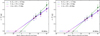 |
Fig. C.1 Distance fit for SN 2013ca using ζBVI as givenin Hamuy et al. (2001; left panel) and Dessart & Hillier (2005; right panel). The diamond markers denote values of χ through which the fit is made. |
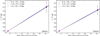 |
Fig. C.2 Distance fit for LSQ13cuw using ζBVI as givenin Hamuy et al. (2001; left panel) and Dessart & Hillier (2005; right panel). The diamond markers denote values of χ through which the fit is made. |
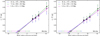 |
Fig. C.3 Distance fit for PS1-13wr using ζBVI as givenin Hamuy et al. (2001; left panel) and Dessart & Hillier (2005; right panel). The diamond markers denote values of χ through which the fit is made. |
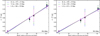 |
Fig. C.4 Distance fit for PS1-12bku using ζBVI as givenin Hamuy et al. (2001; left panel) and Dessart & Hillier (2005; right panel). The diamond markers denote values of χ through which the fit is made. |
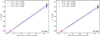 |
Fig. C.5 Distance fit for PS1-13abg using ζBVI as givenin Hamuy et al. (2001; left panel) and Dessart & Hillier (2005; right panel). The diamond markers denote values of χ through which the fit is made. |
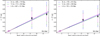 |
Fig. C.6 Distance fit for PS1-13baf using ζBVI as givenin Hamuy et al. (2001; left panel) and Dessart & Hillier (2005; right panel). The diamond markers denote values of χ through which the fit is made. |
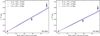 |
Fig. C.7 Distance fit for PS1-13bmf using ζBVI as givenin Hamuy et al. (2001; left panel) and Dessart & Hillier (2005; right panel). The diamond markers denote values of χ through which the fit is made. |
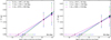 |
Fig. C.8 Distance fit for PS1-13bni using ζBVI as given in Hamuy et al. (2001, left panel) and Dessart & Hillier (2005, right panel). The diamond markers denote values of χ through which the fit is made. Note that this figure shows the last step of the iteration as described in Sect. 3.5.12. |
References
- Anderson, J. P., González-Gaitán, S., Hamuy, M., et al. 2014, ApJ, 786, 67 [NASA ADS] [CrossRef] [Google Scholar]
- Arcavi, I., Gal-Yam, A., Cenko, S. B., et al. 2012, ApJ, 756, L30 [NASA ADS] [CrossRef] [Google Scholar]
- Baltay, C., Rabinowitz, D., Hadjiyska, E., et al. 2013, PASP, 125, 683 [NASA ADS] [CrossRef] [Google Scholar]
- Baron, E., Nugent, P. E., Branch, D., & Hauschildt, P. H. 2004, ApJ, 616, L91 [NASA ADS] [CrossRef] [Google Scholar]
- Bennett, C. L., Larson, D., Weiland, J. L., & Hinshaw, G. 2014, ApJ, 794, 135 [NASA ADS] [CrossRef] [Google Scholar]
- Blondin, S., & Tonry, J. L. 2007, ApJ, 666, 1024 [NASA ADS] [CrossRef] [Google Scholar]
- Bose, S., & Kumar, B. 2014, ApJ, 782, 98 [NASA ADS] [CrossRef] [Google Scholar]
- D’Andrea, C. B., Sako, M., Dilday, B., et al. 2010, ApJ, 708, 661 [NASA ADS] [CrossRef] [Google Scholar]
- de Jaeger, T., González-Gaitán, S., Anderson, J. P., et al. 2015, ApJ, 815, 121 [NASA ADS] [CrossRef] [Google Scholar]
- de Jaeger, T., Galbany, L., Filippenko, A. V., et al. 2017a, MNRAS, 472, 4233 [NASA ADS] [CrossRef] [Google Scholar]
- de Jaeger, T., González-Gaitán, S., Hamuy, M., et al. 2017b, ApJ, 835, 166 [NASA ADS] [CrossRef] [Google Scholar]
- Dessart, L., & Hillier, D. J. 2005, A&A, 439, 671 [NASA ADS] [CrossRef] [EDP Sciences] [Google Scholar]
- Dessart, L., & Hillier, D. J. 2006, A&A, 447, 691 [NASA ADS] [CrossRef] [EDP Sciences] [Google Scholar]
- Eastman, R. G., Schmidt, B. P., & Kirshner, R. 1996, ApJ, 466, 911 [NASA ADS] [CrossRef] [Google Scholar]
- Faran, T., Poznanski, D., Filippenko, A. V., et al. 2014, MNRAS, 445, 554 [NASA ADS] [CrossRef] [Google Scholar]
- Fiorentino, G., Musella, I., & Marconi, M. 2013, MNRAS, 434, 2866 [NASA ADS] [CrossRef] [Google Scholar]
- Freedman, W. L., Madore, B. F., Mould, J. R., et al. 1994, Nature, 371, 757 [NASA ADS] [CrossRef] [Google Scholar]
- Freedman, W. L., Madore, B. F., Gibson, B. K., et al. 2001, ApJ, 553, 47 [NASA ADS] [CrossRef] [Google Scholar]
- Gall, E. E. E., Polshaw, J., Kotak, R., et al. 2015, A&A, 582, A3 [NASA ADS] [CrossRef] [EDP Sciences] [Google Scholar]
- Gall, E. E. E., Kotak, R., Leibundgut, B., et al. 2016, A&A, 592, A129 [NASA ADS] [CrossRef] [EDP Sciences] [Google Scholar]
- González-Gaitán, S., Tominaga, N., Molina, J., et al. 2015, MNRAS, 451, 2212 [NASA ADS] [CrossRef] [Google Scholar]
- Gutiérrez, C. P., Anderson, J. P., Hamuy, M., et al. 2014, ApJ, 786, L15 [NASA ADS] [CrossRef] [Google Scholar]
- Hamuy, M., & Pinto, P. A. 2002, ApJ, 566, L63 [NASA ADS] [CrossRef] [Google Scholar]
- Hamuy, M., Pinto, P. A., Maza, J., et al. 2001, ApJ, 558, 615 [NASA ADS] [CrossRef] [Google Scholar]
- Humphreys, E. M. L., Reid, M. J., Moran, J. M., Greenhill, L. J., & Argon, A. L. 2013, ApJ, 775, 13 [Google Scholar]
- Inserra, C., Smartt, S. J., Gall, E. E. E., et al. 2016, ApJ, submitted, ArXiv e-prints [arXiv:1604.01226] [Google Scholar]
- Jones, M. I., Hamuy, M., Lira, P., et al. 2009, ApJ, 696, 1176 [NASA ADS] [CrossRef] [Google Scholar]
- Kaiser, N., Burgett, W., Chambers, K., et al. 2010, in SPIE Conf. Ser., 7733 [Google Scholar]
- Kirshner, R. P., & Kwan, J. 1974, ApJ, 193, 27 [NASA ADS] [CrossRef] [Google Scholar]
- Landolt, A. U. 1992, AJ, 104, 340 [NASA ADS] [CrossRef] [Google Scholar]
- Leonard, D. C. 2002, PASP, 114, 1291 [NASA ADS] [CrossRef] [Google Scholar]
- Leonard, D. C., Filippenko, A. V., Gates, E. L., et al. 2002a, PASP, 114, 35 [NASA ADS] [CrossRef] [Google Scholar]
- Leonard, D. C., Filippenko, A. V., Li, W., et al. 2002b, AJ, 124, 2490 [NASA ADS] [CrossRef] [Google Scholar]
- Li, W., Leaman, J., Chornock, R., et al. 2011, MNRAS, 412, 1441 [NASA ADS] [CrossRef] [Google Scholar]
- Lilly, S. J., Le Fèvre, O., Renzini, A., et al. 2007, ApJS, 172, 70 [NASA ADS] [CrossRef] [Google Scholar]
- Magnier, E. 2006, in The Advanced Maui Optical and Space Surveillance Technologies Conference, 50 [Google Scholar]
- Maguire, K., Kotak, R., Smartt, S. J., et al. 2010, MNRAS, 403, L11 [NASA ADS] [CrossRef] [Google Scholar]
- Mitchell, R. C., Baron, E., Branch, D., et al. 2002, ApJ, 574, 293 [NASA ADS] [CrossRef] [Google Scholar]
- Nugent, P., Sullivan, M., Ellis, R., et al. 2006, ApJ, 645, 841 [NASA ADS] [CrossRef] [Google Scholar]
- Olivares, E. F., Hamuy, M., Pignata, G., et al. 2010, ApJ, 715, 833 [NASA ADS] [CrossRef] [Google Scholar]
- Pastorello, A., Sauer, D., Taubenberger, S., et al. 2006, MNRAS, 370, 1752 [NASA ADS] [CrossRef] [Google Scholar]
- Pastorello, A., Valenti, S., Zampieri, L., et al. 2009, MNRAS, 394, 2266 [NASA ADS] [CrossRef] [Google Scholar]
- Pejcha, O., & Prieto, J. L. 2015, ApJ, 806, 225 [NASA ADS] [CrossRef] [Google Scholar]
- Perlmutter, S., Aldering, G., Goldhaber, G., et al. 1999, ApJ, 517, 565 [NASA ADS] [CrossRef] [Google Scholar]
- Planck Collaboration, XIII 2016, A&A, 594, A13 [NASA ADS] [CrossRef] [EDP Sciences] [Google Scholar]
- Polshaw, J., Kotak, R., Chambers, K. C., et al. 2015, A&A, 580, L15 [NASA ADS] [CrossRef] [EDP Sciences] [Google Scholar]
- Poznanski, D., Butler, N., Filippenko, A. V., et al. 2009, ApJ, 694, 1067 [NASA ADS] [CrossRef] [Google Scholar]
- Poznanski, D., Nugent, P. E., & Filippenko, A. V. 2010, ApJ, 721, 956 [NASA ADS] [CrossRef] [Google Scholar]
- Poznanski, D., Prochaska, J. X., & Bloom, J. S. 2012, MNRAS, 426, 1465 [NASA ADS] [CrossRef] [Google Scholar]
- Quimby, R. M., Wheeler, J. C., Höflich, P., et al. 2007, ApJ, 666, 1093 [NASA ADS] [CrossRef] [Google Scholar]
- Riess, A. G., Filippenko, A. V., Challis, P., et al. 1998, AJ, 116, 1009 [NASA ADS] [CrossRef] [Google Scholar]
- Riess, A. G., Macri, L., Casertano, S., et al. 2011a, ApJ, 732, 129 [NASA ADS] [CrossRef] [Google Scholar]
- Riess, A. G., Macri, L., Casertano, S., et al. 2011b, ApJ, 730, 119 [NASA ADS] [CrossRef] [Google Scholar]
- Riess, A. G., Macri, L. M., Hoffmann, S. L., et al. 2016, ApJ, 826, 56 [NASA ADS] [CrossRef] [Google Scholar]
- Rodríguez, Ó., Clocchiatti, A., & Hamuy, M. 2014, AJ, 148, 107 [NASA ADS] [CrossRef] [Google Scholar]
- Rubin, A., & Gal-Yam, A. 2016, ApJ, 828, 111 [NASA ADS] [CrossRef] [Google Scholar]
- Sahu, D. K., Anupama, G. C., Srividya, S., & Muneer, S. 2006, MNRAS, 372, 1315 [NASA ADS] [CrossRef] [Google Scholar]
- Sanders, N. E., Soderberg, A. M., Gezari, S., et al. 2015, ApJ, 799, 208 [NASA ADS] [CrossRef] [Google Scholar]
- Schlafly, E. F., & Finkbeiner, D. P. 2011, ApJ, 737, 103 [NASA ADS] [CrossRef] [Google Scholar]
- Schmidt, B. P., Kirshner, R. P., & Eastman, R. G. 1992, ApJ, 395, 366 [NASA ADS] [CrossRef] [Google Scholar]
- Schmidt, B. P., Kirshner, R. P., Eastman, R. G., et al. 1994a, AJ, 107, 1444 [NASA ADS] [CrossRef] [Google Scholar]
- Schmidt, B. P., Kirshner, R. P., Eastman, R. G., et al. 1994b, ApJ, 432, 42 [NASA ADS] [CrossRef] [Google Scholar]
- Takáts, K., & Vinkó, J. 2012, MNRAS, 419, 2783 [NASA ADS] [CrossRef] [Google Scholar]
- Takáts, K., Pumo, M. L., Elias-Rosa, N., et al. 2014, MNRAS, 438, 368 [NASA ADS] [CrossRef] [Google Scholar]
- Tonry, J. L., Stubbs, C. W., Lykke, K. R., et al. 2012, ApJ, 750, 99 [NASA ADS] [CrossRef] [Google Scholar]
- Wagoner, R. V. 1981, ApJ, 250, L65 [NASA ADS] [CrossRef] [Google Scholar]
- Walker, E. S., Hadjiyska, E., Rabinowitz, D., et al. 2013, ATel, 5056, 1 [NASA ADS] [Google Scholar]
- Zhang, K., Wang, X., Zhou, L., et al. 2013, Central Bureau Electronic Telegrams, 3508, 1 [NASA ADS] [Google Scholar]
IRAF (Image Reduction and Analysis Facility) is distributed by the National Optical Astronomy Observatories, which are operated by the Association of Universities for Research in Astronomy, Inc., under cooperative agreement with the National Science Foundation.
SuperNOva PhotometrY, a package for SN photometry implemented in IRAF by E. Cappellaro; http://sngroup.oapd.inaf.it/snoopy.html
Poznanski et al. (2010) give the relation in the form: vFe 5169 = (0.84 ± 0.05) vHβ. We converted this into a vHβ/vFe 5169 ratio for easier comparability with our results.
Throughout this paper we adopt the notation of Gall et al. (2016) in that variables in the SN rest frame will be marked with “⋆”, while “♢” denotes variables in the observer frame.
Large Synoptic Survey Telescope: www.lsst.org
The choice of H0 = 70 km s−1 Mpc−1 is arbitrary and adopted mainly for consistency with the SCM parameters suggested by Nugent et al. (2006). The general principles and our conclusions are the same independent of the exact choice of H0 .
All Tables
All Figures
|
Fig. 1 The SNe in our sample and their environments. Short dashes mark the location of the respective supernova (see Table 1 for the exact coordinates). The images were taken in the SDSS i′ -band on MJD 56 520.89 for SN 2013eq, the i′ -band on MJD 56 462.90 for SN 2013ca, the r′ -band on MJD 56 625.03 for LSQ13cuw, the iPS1 -band on MJD 56 462.31 for PS1-13wr, the i′ -band on MJD 56 768.92 for PS1-14vk, the i′ -band on MJD 56 205.88 for PS1-12bku, the iPS1 -band on MJD 56 422.29 for PS1-13abg, the iPS1 -band on MJD 56 414.52 for PS1-13baf, the iPS1 -band on MJD 56 422.34 for PS1-13bmf, the iPS1 -band on MJD 56 422.29 for PS1-13atm, and the iPS1 -band on MJD 56 432.50 for PS1-13bni. |
| In the text | |
|
Fig. 2 Comparison of Hβ and Fe ii λ5169 velocities. The coloured points correspond to velocities measured between 5 and 40 days from explosion, while the gray points represent epochs either within 5 days of the explosion or after 40 days. The solid lines correspond to the fitted evolution of the Hβ and Fe ii λ5169 velocities for each SN. The green and yellow shaded regions reflect the vH β /vFe 5169 ratios as presented by Nugent et al. (2006) and Poznanski et al. (2010). |
| In the text | |
|
Fig. 3 vHα/vFe 5169 ratio (left panel) and vHβ/vFe 5169 ratio (right panel) compared to the rest frame epoch (from explosion). The thick dotted lines represent the vH α /vFe 5169 and vH β/vFe 5169 ratios for the individual SNe as well as the averaged ratios. For reasons of better visibility the uncertainty is depicted only for the averaged ratios and not for the fitted velocity ratios of the individual SN. Thecircle markers represent the measured vH α /vFe 5169 and vH β/vFe 5169 ratios for those epochs and SNe where spectroscopic data was available and both Hα (or Hβ) and the Fe ii λ5169 velocity could be measured. The yellow shaded band in the right panel corresponds to the ratio of vH β /vFe 5169 = 1.19 |
| In the text | |
|
Fig. 4 Distance fits for PS1-14vk using all available epochs and ζBVI as givenin Hamuy et al. (2001; left panel) and Dessart & Hillier (2005; right panel). The diamond markers denote values of χ through which the fit is made. |
| In the text | |
|
Fig. 5 Distance fits for PS1-14vk using only epochs that follow a linear relation and ζBVI as givenin Hamuy et al. (2001; left panel) and Dessart & Hillier (2005; right panel). The diamond markers denote values of χ through which the fit is made. |
| In the text | |
|
Fig. 6 Comparison of EPM and SCM distances, using the dilution factors by Dessart & Hillier (2005). Filled circles denote SNe with the explosion epoch obtained via EPM, while stars mark SNe with the explosion epoch estimated from pre-discovery photometry. The three Type II-L SNe are labelled specifically. Different colours denote the line that was used to estimate the photospheric velocities: red corresponds to Fe ii λ5169, and dark blue to Hβ. The solid line shows the |
| In the text | |
|
Fig. 7 SN II Hubble diagrams using the distances determined via EPM (left panel) and SCM (right panel). EPM Hubble diagram (left): the distances derived for our sample (circles) use the dilution factors from Dessart & Hillier (2005). The different colours denote the absorption line that was used to estimate the photospheric velocities (Fe ii λ5169 – red; Hβ – blue). We also included EPM measurements from Eastman et al. (1996, E96), Jones et al. (2009, J09) and Bose & Kumar (2014, B14). The solid line corresponds to a ΛCDM cosmology with H0 = 70 km s−1 Mpc−1, Ωm = 0.3 and ΩΛ= 0.7, and the dotted lines to the range covered by an uncertainty on H0 of 5 km s−1 Mpc−1. SCM Hubble diagram (right): circle markers depict the SCM distances derived for our sample using the explosion epochs previously derived via EPM and the dilution factors from Dessart & Hillier (2005). The star shaped markers depict SNe for which an independent estimate of the explosion time was available via photometry. The colours are coded in the same way as for the EPM Hubble diagram. Similarly, the solid and dotted lines portray the same relation between redshift and distance modulus as in the left panel. We also included SCM distances from Poznanski et al. (2009, P09), Olivares et al. (2010, O10) and D’Andrea et al. (2010, A10). We separated the objects “culled” by Poznanski et al. (2009) from the rest of the sample by using a different symbol. The three Type II-L SNe LSQ13cuw, PS1-14vk and PS1-13bmf are identified in both the EPM and the SCM Hubble diagram. |
| In the text | |
|
Fig. A.1 SN 2013ca. Left panel: LT g′ r′ i′ and LSQ V light curves of SN 2013ca. The vertical ticks on the top mark the epochs of the observed spectra. ATel 5056: Walker et al. (2013); CBET 3508: Zhang et al. (2013). Right panel: SN 2013ca spectroscopy. (*) Flux normalized to the maximum Hα flux for better visibility of the features. The exact normalizations are: flux/1.3 for the +30 d spectrum; flux/1.4 for +34 d; flux/1.5 for +46 d; flux/1.5 for +60 d. |
| In the text | |
|
Fig. A.2 PS1-13wr. Left panel: grizyPS1 light curves of PS1-13wr. The vertical ticks on the top mark the epochs of the observed spectra. Right panel: PS1-13wr spectroscopy. (*) Flux normalized to the maximum Hα flux for better visibility of the features. The exact normalizations are: flux/3.4 for the +12 d spectrum; flux/3.5 for +18 d; flux/3.6 for +25 d; flux/3.6 for +41 d. |
| In the text | |
|
Fig. A.3 PS1-14vk. Left panel: LT g′ r′ i′ light curves of PS1-14vk. The vertical ticks on the top mark the epochs of the observed spectra. Right panel: PS1-14vk spectroscopy. (*) Flux normalized to the maximum Hα flux for better visibility of the features. The exact normalizations are: flux/2.6 for the +2 d spectrum; flux/2.7 for +11 d; flux/2.8 for +14 d; flux/2.3 for +27 d; flux/2.1 for +33 d; flux/1.9 for +49 d. |
| In the text | |
|
Fig. A.4 PS1-12bku. Left panel: grizyPS1 and NOT u′g′r′i′z′ light curves of PS1-12bku. The vertical ticks on the top mark the epochs of the observed spectra. Right panel: PS1-12bku spectroscopy. (*) Flux normalized to the maximum Hα flux for better visibility of the features. The exact normalizations are: flux/3.3 for the +23 d spectrum; flux/3.6 for +27 d; flux/3.5 for +41 d; flux/2.9 for +81 d. |
| In the text | |
|
Fig. A.5 PS1-13abg. Left panel: grizyPS1 light curves of PS1-13abg. The vertical ticks on the top mark the epochs of the observed spectra. Right panel: PS1-13abg spectroscopy. (*) Flux normalized to the maximum Hα flux for better visibility of the features. The exact normalizations are: flux/0.7 for the +7 d spectrum; flux/0.8 for +32 d; flux/1.1 for +44 d. |
| In the text | |
|
Fig. A.6 PS1-13baf. Left panel: grizyPS1 light curves of PS1-13baf. The vertical ticks on the top mark the epochs of the observed spectra. Right panel: PS1-13baf spectroscopy. (*) Flux normalized to the maximum Hα flux for better visibility of the features. The exact normalizations are: flux/4.1 for the +16 d spectrum; flux/3.2 for +28 d; flux/2.9 for +39 d. |
| In the text | |
|
Fig. A.7 PS1-13bmf. Left panel: grizyPS1 light curves of PS1-13bmf. The vertical ticks on the top mark the epochs of the observed spectra. Right panel: PS1-13bmf spectroscopy. (*) Flux normalized to the maximum Hα flux for better visibility of the features. The exact normalizations are: flux/5.7 for the +5 d spectrum; flux/9.5 for +8 d; flux/8.8 for +29 d; flux/5.1 for +47 d. |
| In the text | |
|
Fig. A.8 PS1-13atm. Left panel: grizyPS1 light curves of PS1-13atm. The vertical ticks on the top mark the epochs of the observed spectra. Right panel: PS1-13atm spectroscopy. (*) Flux normalized to the maximum Hα flux for better visibility of the features. The exact normalizations are: flux/4.3 for the +16 d spectrum; flux/6.1 for +23 d; flux/7.8 for +44 d. |
| In the text | |
|
Fig. A.9 PS1-13bni. Left panel: grizyPS1 light curves of PS1-13bni. The vertical ticks on the top mark the epochs of the observed spectra. Right panel: PS1-13bni spectroscopy. (*) Flux normalized to the maximum Hα flux for better visibility of the features. The exact normalizations are: flux/2.5 for the +14 d spectrum; flux/2.5 for +15 d; flux/2.5 for +24 d; flux/2.2 for +32 d; flux/2.1 for +51 d. |
| In the text | |
|
Fig. C.1 Distance fit for SN 2013ca using ζBVI as givenin Hamuy et al. (2001; left panel) and Dessart & Hillier (2005; right panel). The diamond markers denote values of χ through which the fit is made. |
| In the text | |
|
Fig. C.2 Distance fit for LSQ13cuw using ζBVI as givenin Hamuy et al. (2001; left panel) and Dessart & Hillier (2005; right panel). The diamond markers denote values of χ through which the fit is made. |
| In the text | |
|
Fig. C.3 Distance fit for PS1-13wr using ζBVI as givenin Hamuy et al. (2001; left panel) and Dessart & Hillier (2005; right panel). The diamond markers denote values of χ through which the fit is made. |
| In the text | |
|
Fig. C.4 Distance fit for PS1-12bku using ζBVI as givenin Hamuy et al. (2001; left panel) and Dessart & Hillier (2005; right panel). The diamond markers denote values of χ through which the fit is made. |
| In the text | |
|
Fig. C.5 Distance fit for PS1-13abg using ζBVI as givenin Hamuy et al. (2001; left panel) and Dessart & Hillier (2005; right panel). The diamond markers denote values of χ through which the fit is made. |
| In the text | |
|
Fig. C.6 Distance fit for PS1-13baf using ζBVI as givenin Hamuy et al. (2001; left panel) and Dessart & Hillier (2005; right panel). The diamond markers denote values of χ through which the fit is made. |
| In the text | |
|
Fig. C.7 Distance fit for PS1-13bmf using ζBVI as givenin Hamuy et al. (2001; left panel) and Dessart & Hillier (2005; right panel). The diamond markers denote values of χ through which the fit is made. |
| In the text | |
|
Fig. C.8 Distance fit for PS1-13bni using ζBVI as given in Hamuy et al. (2001, left panel) and Dessart & Hillier (2005, right panel). The diamond markers denote values of χ through which the fit is made. Note that this figure shows the last step of the iteration as described in Sect. 3.5.12. |
| In the text | |
Current usage metrics show cumulative count of Article Views (full-text article views including HTML views, PDF and ePub downloads, according to the available data) and Abstracts Views on Vision4Press platform.
Data correspond to usage on the plateform after 2015. The current usage metrics is available 48-96 hours after online publication and is updated daily on week days.
Initial download of the metrics may take a while.