© ESO 2018

1 Introduction

In the star-forming disks of spiral galaxies the dominant source of turbulence at scales of 10–100 pc is provided by supernova (SN) explosions (e.g. Abbott 1982). Releasing both thermal and kinetic energy into the ambient interstellar medium (ISM), the SNe generate vigorously turbulent flows with an average Mach number close to unity (van Weeren et al. 2016), and with local values even higher (Heiles & Troland 2003). SN forcing has interesting properties. Firstly, in homogeneous media, each explosion is initially purely potential, meaning that in the radially expanding shock fronts vorticity vanishes while divergence is non-zero. Such high Mach number flows with strong compression are expected to show steep power laws in their energy spectra (compressible spectra with spectral slope − 2, solenoidal spectra with − 3; see e.g. Vazquez-Semadeni et al. 1995, and references therein). However, the observed spectrum of ISM turbulence is close to that of Kolmogorov turbulence (Armstrong et al. 1981, 1995), so the overall interstellar flow generated by an ensemble of SNe appears to contain significant vorticity. Although this issue has gained some attention in the past (Chernin 1996; Vazquez-Semadeni et al. 1995; Korpi et al. 1999b; Balsara et al. 2004; Mee & Brandenburg 2006; Del Sordo & Brandenburg 2011; Padoan et al. 2016), a systematic investigation of vorticity generation in SN-forced flows including all relevant ingredients (rotation, shear, full thermodynamics, density stratification) is so far lacking. Such an investigation is attempted here.

SN forcing acts on the stratified flows with rotation and shear, providing suitable conditions for the production of net helicity. These effects, in addition to the presence of a large-scale magnetic field, also make the flow anisotropic. The presence or absence of net helicity has strong implications for vortex generation, and also for the galactic dynamo mechanism. Net helicity, through the effect of the Coriolis force on the expanding bubbles, enables amplification of magnetic fields (the α-effect). In its absence, the dynamo must rely on other shear- or rotation-induced effects or instabilities. For example, magnetorotational instability (MRI) arises due to the presence of weak magnetic fields in a system subject to large-scale shear (see e.g. Sellwood & Balbus 1999; Piontek & Ostriker 2005, 2007). Also, purely stochastic turbulence (see e.g. Singh 2016) can lead to large-scale dynamo action.

A second interesting property of SN forcing is that it can be regarded as a random, external forcing. In such a system, there is a preferential frame of reference, under which forcing is defined; hence breaking Galilean invariance. Under such conditions, the velocity field can be de-stabilised at large scales analogous to the dynamo α-effect, as first proposed by Moiseev et al. (1983) for compressible fluids, resulting in the generation of mean flows and thereby also vorticity. For the incompressible case, such an effect is only possible if the forcing is anisotropic, as discussed by Krause & Rüdiger (1974). Frisch et al. (1987) called this effect the anisotropic-kinetic-α effect, later referred to as the AKA effect. So far it has been detected only in rather simple and idealised models, requiring specialised forcing functions in direct numerical simulations (see e.g. Brandenburg & von Rekowski 2001; Levina & Burylov 2006), although it has been verified using mean-field models in realistic setups (see e.g. von Rekowski et al. 1995). The analytical study of Pipin et al. (1996) showed that this effect can be expected only at moderate Coriolis number (i.e. flows with moderate rotational influence). The numerical study of Brandenburg & von Rekowski (2001) indicated that the effect would only be possible in flows with low Reynolds number, at least for the specific forcing function considered, which injected helicity through a forcing profile moving with the flow. The astrophysical significance of this effect, therefore, remains unclear.

Many approaches have been developed and implemented to realistically simulate ISM turbulence (e.g. Rosen et al. 1996; Korpi et al. 1999a; de Avillez & Breitschwerdt 2005; Mac Low et al. 2005; Gent et al. 2013a) and galactic dynamo action (e.g. Gressel et al. 2008; Hanasz et al. 2009; Gent et al. 2013b). These routinely report significant amounts of vorticity and net helicity, but to date systematic studies of the mechanisms responsible for their generation have only been made in far simpler settings (Vazquez-Semadeni et al. 1995; Balsara et al. 2004; Mee & Brandenburg 2006; Del Sordo & Brandenburg 2011), except for the tentative study of Korpi et al. (1999b) and the recent investigation by Padoan et al. (2016). In the latter, however, rotation and shear were excluded. Both identified the baroclinicity as an important driver of vorticity, but a systematic study of all the other possible sources of vorticity was not undertaken. The conditions which violate the Kelvin–Helmholtz theorem for the conservation of vorticity in the astrophysical context – specifically viscosity, shocks, baroclinicity and helical forcing – are discussed extensively by Chernin (1996). All are present in ISM turbulence, but whether in a given system each leads to the generation or destruction of vorticity must still be determined.

The large-scale shear can also affect the SN forced flow in various ways. In addition to taking part in the dynamo process by shearing out any radial magnetic field to efficiently produce azimuthal field, it can also drive mean helicity and, thereby, a shear-induced α-effect in the evolution equation of the magnetic field, as proposed by, for example, Rogachevskii & Kleeorin (2003) and Rädler & Stepanov (2006).

Further, shear can be argued to make the flow highly anisotropic, reasoning as follows. Under the local shearing sheet approximation used in many studies, the linear shear will cause the turbulent cells to elongate. In our case the linear shear in the radial x direction elongates the cells in the azimuthal y direction; this can be approximated as $$H=\text{vect}u\cdot \overrightarrow{\omega }$$

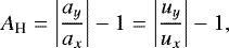
where τ is the lifetime of turbulent cells and $H=\text{vect}u\cdot \overrightarrow{\omega }$ is the shear flow, with S the shear parameter r∂Ω∕∂r. Stepanov et al. (2014) and Hollins et al. (2017) adopt a similar approach to estimate the shear-induced magnetic field anisotropy. For flat rotation curves in galaxies S = −qΩ, with q = 1. We define a parameter describing the anisotropy of the horizontal components of the turbulent velocity field, u^′, as $$H=\text{vect}u\cdot \overrightarrow{\omega }$$(1)

where ${u^{\prime }}_{i,\text{rms}}$ denotes the volume- and time-averaged rms-value of the turbulent velocity component (see Sect. 2 for formal definitions of our notations for averages). We note that allowing only for shear, A_H > 0 (l_y > l_x). With both shear and rotation present, A_H < 0 (l_x > l_y) is possible; the combined effects of shear and rotation on anisotropy are considered in Sect. 3.1.

Analogously, density stratification along the z-coordinate causes an anisotropy, that is, a difference between the vertical and radial turbulent velocities, which can similarly be estimated as $$H=\text{vect}u\cdot \overrightarrow{\omega }$$(2)

where U_z is the typical velocity of the gas flow from the disc to the halo and l_x is the radial scale of turbulence. In deriving the ratios of rms velocities in these estimates, we have assumed that the velocity field can be approximated as being incompressible, ∇ ⋅ u = 0. Although this assumption only applies at limited transitory positions, since the Mach number averaged over the whole computational domain is commonly slightly above unity, it is still instructive to proceed.

Estimates typical for the solar neighbourhood are S ≃ −25 km s−1 kpc⁻¹, τ ≃ 5 × 10⁶ yr (Hollins et al. 2017), U_z ≃ 100 km s−1 (Gent et al. 2013a) and l_x ≃ 100 pc (e.g. Korpi et al. 1999a). Thus, one arrives at estimates A_H ≃ 0.15 and A_V ≃ 5.

Finally, the shear can cause instabilities in the ISM, one of the most interesting being the MRI, also capable of sustaining dynamo action through the turbulence it generates and maintains (see e.g. Brandenburg et al. 1995). It has been argued that the turbulent mixing due to SNe can suppress the instability (e.g. Korpi et al. 2010; Gressel et al. 2013). No definite signs of MRI have been observed in any of the SN-driven ISM simulations thus far (e.g. Korpi et al. 1999a; Gressel et al. 2008), although separating its effect from the other sources of turbulence and magnetic fields is a challenging task (see, e.g. Korpi et al. 2010). By estimating the values of turbulent diffusivity resulting from SN activity, one can estimate the likelihood of its presence, an approach adopted in this paper to refine earlier estimates of (Korpi et al. 2010).

We begin by estimating the magnitude of the anisotropy parameters resulting from the shear flows and density stratification and comparing them to the expected values (Sect. 3.1). Next we discuss the various vorticity generation mechanisms in the system (Sect. 3.2). We continue by measuring the net kinetic helicity, and separating the contributions due to rotation and shear by using rotation laws with opposite shear parameters q (Sect. 3.3). Section 3.4 concentrates on investigating the possible sources of the oscillatory mean flows generated in the system. We quantify the AKA effect αand turbulent viscosity in the flow using the method of moments (Brandenburg & Sokoloff 2002). In Sect. 3.5 we use the diffusivity estimate to refine the prediction for the existence of MRI in the system.

2 Model

We numerically model a three-dimensional (3D) region of the ISM situated within a galactic disk, described in detail by Gent et al. (2013a, hereafter Paper I), and Gent (2012,Part II). The computational domain spans 1.024 kpc horizontally and ± 1.12 kpc vertically, centred on the galactic plane. Resolution along each edge is 4 pc . Model Cartesian coordinates (x, y, z) are the analogue of galactic cylindrical coordinates (r, ϕ, z), respectively.A snapshot of the model is illustrated in Fig. 1. An existing simulation from Paper I with mean gas number density 1.2 cm−3 at the midplane in a non-rotating frame is used as the initial turbulent condition. Runs apply varied differential rotation profiles, implemented via a shearing periodic boundary in the x-direction.

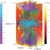Fig. 1 Representative snapshot from Run 1Ωp with contours on the top, bottom, and back surfaces of the simulation box indicating the ISM temperature (red-yellow), and isosurfaces within the box indicating the gas density (purple-cyan). Streamlines of velocity (green) are plotted through the isosurfaces.

A system of compressible hydrodynamical (HD) equations are solved using the Pencil Code¹ , applying sixth-order finite differences for spatial vector operations and a third-order Runge-Kutta scheme for integration over time. The basic equations include the mass conservation, Navier-Stokes and the energy equations, the latter written in terms of specific entropy: $$\frac{D\rho }{Dt}=-\rho \overrightarrow{\nabla }\cdot \overrightarrow{u}+{\dot{\rho }}_{\text{SN}},$$(3) $$\text{begin}align*\frac{D\overrightarrow{u}}{Dt}\text{}\text{}\text{\&}=\text{ \&}\text{}\text{}-c_{\text{s}}^2\overrightarrow{\nabla }\left(\frac{s}{c_p}+\text{ln}\rho \right)+\overrightarrow{g}-S{u}_x\text{bm}\widehat{y}-2\overrightarrow{\text{UpOmega}}\times \overrightarrow{u}\text{nn nn \&\&}+\nu {\nabla }^2\overrightarrow{u}+\frac{\nu }{3}\overrightarrow{\nabla }\overrightarrow{\nabla }\cdot \overrightarrow{u}+2\text{ bm}S\cdot \left(\nu \overrightarrow{\nabla }\text{ln}\rho +\overrightarrow{\nabla }\nu \right)+{\zeta }_{\nu }\left(\overrightarrow{\nabla }\overrightarrow{\nabla }\cdot \overrightarrow{u}\right),T\frac{Ds}{Dt}\text{}\text{}\text{ \&}=\text{\&}\text{}\text{}\frac{{\dot{\sigma }}_{\text{SN}}}{\rho }+\Gamma -\rho \Lambda +\frac{c_p}{\rho }\overrightarrow{\nabla }\cdot \chi \rho \overrightarrow{\nabla }T+2\nu \text{ bm}{S}^2+T\overrightarrow{\nabla }{\zeta }_{\chi }\cdot \overrightarrow{\nabla }s,\text{end}align*$$

where ρ, T, and s are the gas density, temperature, and specific entropy, respectively. The gas velocity u (here called the velocity perturbation) is the deviation from the background rotation and shear flow profile, but contains some horizontal and vertical mean flows showing dependence on the vertical coordinate. Gravitational acceleration is g, adiabatic speed of sound c_s, and heat capacity at constant pressure c_p . The velocity shear rate S is associated with the galactic differential rotation at the angular velocity Ω = (0, 0, Ω) (see below). Stellar heating and gas cooling by radiation are denoted by Γ and Λ, respectively.Viscosity ν and thermal diffusivity χ apply proportionally to the local sound speed, and shock capturing diffusivities ζ_ν and ζ_χ apply where flows converge. The advective derivative, $$\frac{D\overrightarrow{}}{Dt}=\frac{\partial }{\partial t}+\left({\overrightarrow{u}}_0+\overrightarrow{u}\right)\cdot \overrightarrow{\nabla },$$

includes the transport by the imposed shear flow u₀ = (0, S x, 0). Viscous stress and heating involve the rate of strain tensor S, $$2S_{ij}=\frac{\partial u_i}{\partial x_j}+\frac{\partial u_j}{\partial x_i}-\frac{2}{3}{\delta }_{ij}\overrightarrow{\nabla }\cdot \overrightarrow{u},\text{with}\text{bm}{S}^2\equiv S_{ij}{S}_{ij}.$$

We adopt a gravitational acceleration, g = (0, 0, −g_z), due to an external gravitational potential including the stellar and dark-matter components as derived by Kuijken & Gilmore (1989)² $$g_z=\frac{a_{\text{s}}z}{\sqrt{z_{\text{s}}^2+z^2}}+\frac{a_{\text{d}}z}{z_{\text{d}}},$$(6)

with a_s = 4.4 × 10⁻¹⁴ km s⁻², a_d = 1.7 × 10⁻¹⁴ km s⁻², z_s = 200 pc and z_d = 1 kpc (Korpi et al. 1999a; Ryan Joung & Mac Low 2006; de Avillez & Breitschwerdt 2007; Gressel et al. 2008; Bendre et al. 2015, and also Paper I). For the equation of state we adopt the ideal gas law $$p=\frac{k_{\text{B}}}{\mu m_{\text{u}}}\rho T,$$(7)

where k_B denotes theBoltzmann constant, m_u the atomic mass unit and μ the mean molecular weight, for which we adopt the value 0.531 corresponding to fully ionised gas of the ISM in the solar neighbourhood³.

In common with the approach of other authors, we locate SN remnants as spherical regions, into which we add 10⁵¹ erg of thermal energy (σ_SN) and mass equivalent to 10 M_⊙ (ρ_SN). For more details on the SNe scheme, rate and distribution, we refer to Paper I. For the current simulations, kinetic energy injection is no longer included and improved time step control negates any requirement for suppressing cooling or heating in shocks (Gent 2012, Appendix A.2). To conserve the characteristics of the turbulence in the long term, the SN rate is proportional to the mean gas density, so there are quasi-regular inflows and outflows. In Paper I the SN rate was fixed and the turbulence was characterised by continual net outflows.

The complicated radiative cooling processes are essential to the ISM structure and dynamics. Their qualitative cumulative impact is parameterised by a simple power-law hybrid of forms derived by Wolfire et al. (1995) and Sarazin & White (1987), listed in Table 1 of Paper I (see also Gressel et al. 2008; Gent et al. 2013b; Bendre et al. 2015; Paper I); it takes the form Λ = Λ_kT^β_k, applicable at temperatures in discrete ranges T_k ≤ T < T_k+1. UV heating follows Wolfire et al. (1995), with 0.015 erg g⁻¹ s⁻¹ vanishing smoothly for T ≳ 10⁴ K ⁴.

Spiral galaxies typically have almost flat rotation curves: the angular velocity has the form Ω ∝ r⁻¹, and the shear parameter S ∝−Ω. It is convenient to consider the ratio, q, of the shear parameter to the rotation rate, defined as $$q=-\frac{S}{\text{UpOmega}}\cdot$$(8)

For known galaxies the outer disk rotates more slowly than the inner disk, that is, q is positive. In this study, we also consider q < 0, clearly bearing no astrophysical relevance, but with the intention of distinguishing the rotation- and shear-induced contributions to net kinetic helicity $H=\text{vect}u\cdot \overrightarrow{\omega }$, as explained in detail in Sect. 3.3. The Rayleigh instability is present only when q > 2, so all runs included are known to be hydrodynamically stable. In the magnetohydrodynamic (MHD) regime runs with normal galactic rotation profiles would, however, be subject to MRI for all q > 0. We normalise Ω and S, with respect to Ω₀ = 25 km s−1 kpc⁻¹, that is, the angular velocity of our Galaxy in the solar neighbourhood. Runs are listed in Table 1, with “p” or “n” in labels indicative of positive or negative q, respectively, and numbers indicative of multiples of Ω₀.

We measure the relative strength of rotation and shear with the Coriolis and shear numbers, respectively, $$H=\text{vect}u\cdot \overrightarrow{\omega }$$(9)

where l₀ is a typical length scale of the turbulence, and $u_{\text{rms}}^{\prime }$ is the volume- and time-averaged rms turbulent velocity averaged over domain and duration for each simulation. Here the turbulent (or random) flow u^′ is calculated as $\text{vect}{u}^{\prime }=\text{vect}u-\overline{\text{vect}u}$, where $\overline{\text{vect}u}$ is the mean flow obtained from horizontal averages of the perturbation velocity u. The vigor of turbulence with respect to viscous effects is measured by the Reynolds number $$\text{Re}=\frac{u_{\text{rms}}^{\prime }{L}_x}{\nu },$$(10)

where we have used the horizontal extent of the box (L_x ) as the length scale. The viscosity in our model is set proportional to the local sound speed; see Paper I for details.

The molecular viscosity for fully ionised gas follows the Spitzer form: ν ∝ ρ⁻¹T^5∕2 (Spitzer 1956; Brandenburg & Subramanian 2005, Sect. 3). ISM model temperature varies by up to seven orders of magnitude. In stellar convection, increased viscosity at high temperatures is at least partially offset by correlated increases in density, but in the hot ISM, Spitzer viscosity is further amplified by the reduced density. Such large viscous forces applying in the hottest regions of the ISM may reduce the timestep to the extent that it becomes numerically impractical. Whether Spitzer constant, or any other viscosity prescription is more realistic for such turbulent viscosities is unknown, and our method confers sufficient viscosity to resolve hot regions with high sound speeds, while applying considerably less viscosity to flows with lower temperatures. When calculating the Reynolds numbers, we use the volume- and time-averaged adiabatic rms sound speed to estimate the viscosity for the model in question, that is, $\nu ={\nu }_0\text{ left}<T^{1/2}\text{right}>$, where ν₀ = 0.004 kpc km s−1 K^−1∕2. The Prandtl number, Pr = ν∕χ ≃ 6–7. Studies of the hot intracluster medium (Gaspari & Churazov 2013) suggest Pr ~ 100, and Pr values for the ISM are likely of the same order of magnitude. While this is beyond the limits of our numerical scheme, Pr > 1 is at least tending towards the correct regime.

We require various averaging procedures to represent our results. We approximate ensemble averages by volume- and time-averaged rms values, as computing fully consistent ensemble averages from a large number of independent realisations of the system state is computationally prohibitively expensive. These are defined and denoted as $$f_{\text{rms}}=\text{sqrt{left}<f^2\text{ right}>\text{}},$$(11)

where f is either a scalar or vector field, and angular brackets $\text{left}<\cdot \text{right}>$ denote the mean over the whole computational volume and time.

Horizontal averages, with the averaging being performed over the horizontal x and y directions, are denoted with overbars, resulting in z-dependent profiles of the horizontal means. Where the z-dependent mean is non-zero, turbulent quantities are given by $$f^{\prime }=f-\overline{f},$$(12)

from which the rms quantities can then be computed. Furthermore, time-averaged horizontal averages are denoted with ${\overline{(f)}}_{\text{t}}$.

In Sect. 3.4, we also consider z- and t-averages (applied to quantities which are already horizontal averages): we denote those operations by ${\langle \cdot \rangle }_z$ and ${\langle \cdot \rangle }_{\text{t}}$, respectively.

3 Results

We performed seven runs, for which distinguishing input parameters and some indicative output diagnostics are listed in Table 1. Our strategy is to examine the influence of variation in rotation and shear on the properties of the flow, while fixing the magnitude of their ratio, q. The sign of this parameter defines whether the rotational velocity decreases (positive) or increases (negative) as a function of radius, and also whether the shear acts against (with) rotation. Run 1Ωp has the parameter set best representing the solar neighbourhood of the Milky Way, while Runs 2Ωp and 4Ωp have, respectively, twice and four times the rotation and shear rates. Runs 1Ωn, 2Ωn , and 4Ωn are the same, but with the sign of rotation, and hence the sign of q, reversed. For reference, we also include Run 0Ω0 without any rotation or shear. All runs are integrated for 300 Myr during a statistical steady state; 8–16 turnover times each, given turnover times, $t_{\text{to}}=L_x/u_{\text{rms}}^{\prime }$, in the range19–38 Myr.

In Fig. 1 we show a typical snapshot from Run 1Ωp, presenting its density, temperature, and velocity fields together. We see the most cold, dense gas gathered near the midplane, while the hot and warm structures dominate away from it. However, these regions persist in close proximity, with the cold gas having a very small filling factor. The supernova remnants appear as bubbles of hot dilute gas of very irregular shapes, and are also apparent in the velocity field. The latter has an irregular structure, with the streamlines more horizontal near the SN-dominated midplane, while vertical flows become visible at heights. Due to the continuous, dynamical adjustment of the disk stratification with SN activity, systematic vertical oscillations occur. These oscillations are quasi-regular, on a time scale somewhat longer than the turnover time, and all our simulations cover at least three such cycles (see Sect. 3.4).

In Table 1 we list volume- and time-averages of the root-mean-square perturbation velocity u_rms (excluding u₀ ), and the fluctuating equivalent u′rms (with any generated mean flow also excluded), as well as the vorticity, ωrms. In addition to the mean vertical flows, unexpectedly, there are also horizontal z-dependent flows generated in all runs where rotation and shear are present. We devote Sect. 3.4 to understanding the generation of these mean flows. Another general observation, given Coriolis and shear numbers |Co | = 2|Sh| < 1 (see Table 1) even at the highest rotation rates investigated, is that the SN-driven velocity fluctuations dominate over rotation and shear.

As the SN rate is dependent on mean density, the SN energy input is varying somewhat between the different runs; hence we list it as an output diagnostic in Table 1. Most of the energy is retained in the form of thermal energy E_th , with a somewhat smaller amount in the kinetic energy of the gas motions E_kin: on average 60% of the thermal energy across all runs. Over the whole domain and duration of each run, the systems contain on average the energy of about 50 SNe, while the total energy input throughout a typical simulation run is near 6 × 10³ σ_SN. Only some fraction of this energy is used to stir and heat the ISM as it is advected away from the disk or lost to radiative processes, as parameterised in the cooling function.

In the early stage of a SN explosion in the model, bubbles of hot gas are created. The imbalance between the high thermal pressure explosion site and the lower pressure ambient medium drives an expanding shock front. If such expansion happens in a homogeneous medium, the resulting flow is purely divergent (potential) and has no vorticity (rotational component). Seeking a Helmholtz decomposition of the flow in each snapshot into its potential and rotational parts, we contract the 3D Fourier transform of the flow and the wave vector, $\widehat{\text{vect}u}(\text{vect}k)\cdot \text{vect}k$, to derive the potential flow ${\widehat{\text{vect}u}}_{\text{pot}}$. From this we obtain $H=\text{vect}u\cdot \overrightarrow{\omega }$. The volume integrals of these flows satisfy $\langle |\text{vect}u{|}^2\rangle =\langle |\text{vect}{u}_{\text{pot}}{|}^2\rangle +\langle |\text{vect}{u}_{\text{rot}}{|}^2\rangle ,$

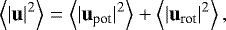
where these terms denote the square of the Euclidian norm⁵ of each field. In spite of the potential forcing, from Table 2, we observe in all models that the volume and time averaged squared norm of the rotational flow, $u_{\text{rot}}^2$, is not only non-zero, but more substantial than that of the potential flow, $u_{\text{pot}}^2$. Due to strong temporal variation the potential flow is occasionally dominant, persisting up to a few Myrs as such in models 4Ωp and 0Ω0.

The kinetic energies arising from these flows, listed in Table 2, satisfy $$\langle \rho |\text{vect}{u}_{\text{pot}}{|}^2\rangle +\langle \rho |\text{vect}{u}_{\text{rot}}{|}^2\rangle >\langle \rho |\text{vect}u{|}^2\rangle ,$$

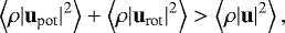
and we can observe near parity between E_pot and E_rot, although the latter is still the more substantial. The physical interpretation of these quantities will be considered more closely in a future work, which will also discuss in detail the implementation of Helmholtz decomposition in a highly compressible system with open boundaries. For the current study it is sufficient to note the dominant proportion of rotational flow in all models.

The generation of rotational modes in the non-rotating, non-shearing Run 0Ω0 is a clear indication that this mechanism cannot be solely related to rotation and shear acting on the system. This conclusion is further reinforced by the evidence that the energy fraction is changing only mildly between the runs where the magnitudes of these effects differ significantly. These observations point to there being a special property of the SN forced flow itself, that leads to the dominance of rotational modes. This issue is discussed in detail in Sect. 3.2.

Investigating the system by segregation into phases often proves more informative than investigating it as a whole. Much previous work has focussed specifically on the diffuse ionised gas, for which observational tools are relatively well suited (Reynolds 1977, 1991; Kulkarni & Heiles 1988; Berkhuijsen et al. 2006; Gaensler et al. 2008) and the possibility of clearly distinguishing the properties of this phase from the broader ISM aids interpretation of the data. In Paper I the hydrodynamical properties of the ISM phases are investigated in depth, and Evirgen et al. (2017) analyse the structure of the magnetic field in the warm and hot phases to assist interpretation of galactic magnetic field observations (Rand & Kulkarni 1989; Beck et al. 1996; Haverkorn 2015).

Here some relevant diagnostics by phase are listed in Table 3 for Runs 1Ωp, 2Ωp, and 4Ωp, which reveal that the rotation and shear influences are only significant (Co ≥ 1) in the cold and warm phases and only for Run 4Ωp, and are weak in the hot phase, and in all phases for Runs 1Ωp and 2Ωp. This conclusion could have been reached simply by investigating the timescales of various effects, at least for the full simulated ISM: in the solar neighbourhood, the rotational (and shearing) time scale is about 250 Myr, an order of magnitude larger than the turnover time of turbulence on average over all phases.

Comparing the vorticity for the full ISM in Table 1, with each phase in Table 3, it is clear that the largest contribution to vorticity comes from the hot phase both in absolute terms but also when normalised with the typical rms velocities and length scales in each phase (the numbers given in brackets). This indicates that even the vorticity generation mechanisms may be distinct by phase in a SN-regulated system. We also note from Table 3 that antisymmetry of helicity about the midplane is evident in both the warm and hot phases; that is, the helicity is clearly negative (positive) in the upper (lower) half-spaces, as is expected for positive values of Ω. As we observe from Table 4, the sign rule is reversed for negative Ω. The cold phase does not show any systematic trend. As for the full ISM (shown later in Table 4), the fluctuations in helicity are significantly larger than their mean values.

3.1 Anisotropies

In this section we concentrate on investigating the level of horizontal and vertical anisotropies in the system. For this purpose, we have computed these quantities, listed in Table 1, using the definitions introduced in Eqs. (1) and (2), $$\text{begin}align*\text{nn\&}{A}_{\text{H}}=\frac{{u^{\prime }}_{y,\text{rms}}}{{u^{\prime }}_{x,\text{rms}}}-1,\text{nn\&}{A}_{\text{V}}=\frac{{u^{\prime }}_{z,\text{rms}}}{{u^{\prime }}_{x,\text{rms}}}-1,\text{end}align*$$

with ${u^{\prime }}_{i,\text{rms}}$ as defined by Eqs. (11) and (12). We note that, in contrast to the shear-only situation considered in the Introduction, the full system contains both shear and rotation; in which case, both signs of A_H are possible.

As expected, horizontal anisotropy vanishes for Run 0Ω0 with neither shear nor rotation. For runs with q = 1, hereafter referred to as the positive q branch, A_H is weakly negative and increasing in magnitude with Ω and S, maximal magnitudes being of order − 0.1. For runs with q = −1, hereafter referred to as the negative q branch, A_H is positive, also increasing with Ω and S, the maximal magnitude being about twice that of the positive q branch. We can make two interesting observations. First, all A_H values obtained are much smaller in magnitude than expected from Eq. (1) with typical Galactic parameters. Second, there is an asymmetry with respect to the magnitude of A_H between the branches: the x (radial) component is dominant (sub-dominant) to the y (azimuthal) component on the positive (negative) q branch. Furthermore, the rate of the magnitude increase is lower (higher) on the positive (negative) branch.

A large part of the asymmetry between the different q branches can be explained by considering the effects of shear and rotation in the system, illustrated schematically in Fig. 2. As the change of sign of q is achieved by reversing the sign of Ω, the contribution from the shear flow to the time-derivative of azimuthal velocity, qΩu_x, is positive for both branches of q. On the positive branch, the contribution from the Coriolis force to the time-derivative of u_y is − 2Ωu_x (which acts in opposition to the shear influence on this azimuthal velocity), while the contribution to the time-derivative of u_x is 2Ωu_y (which acts in the same direction as the shear). Therefore, the dominance of the radial velocity component and a negative sign of A_H is expected. On the negative q branch, the sign of Ω reverses, so the rotational contributions to both flow components also reverse sign. In that regime, therefore, the shear and rotation both act to add to u_y, which explains its dominance and the positive sign of A_H on this branch.

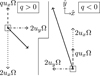Fig. 2 A schematic picture illustrating how the Coriolis and shearing components of the flow influence AH , for positive and negative q (here drawn assuming that ux and uy are positive, with Ω the magnitude of rotation, |Ω|, and for |q| = 1).

The simple estimate, Eq. (1), only accounts for the effect of the large-scale shear, which in this system always adds to the azimuthal velocity component, as illustrated in Fig. 2. The Coriolis force due to rotation provides a larger contribution to the horizontal anisotropy than the shear, however (although we note that the Coriolis force on its own would not produce any anisotropy; it is the combination of rotation and shear that is important). As a result, with the parameters describing the solar neighbourhood in the Milky Way on the physical q = 1 branch, we obtain a dominant radial velocity component, indicating a negative horizontal anisotropy parameter.

This can clearly be seen from considering the contributions to the evolution equations for u_x and u_y associated with rotation and shear: a_x = ∂u_x∕∂t = 2Ωu_y, a_y = ∂u_y∕∂t = −Su_x − 2Ωu_x = (q − 2)Ωu_x, using S = −qΩ. Defining A_H as $$A_{\text{H}}=\left|\frac{a_y}{a_x}\right|-1=\left|\frac{u_y}{u_x}\right|-1,$$(15)

this then results in a quadratic equation for A_H . With only the rotation and shear terms present, the timescales of the x- and y-components are the same, so the definitions via the components of a and u are equivalent. Excluding the non-physical root, this gives $$A_{\text{H}}=\frac{\sqrt{2(2-q)}}{2}-1,$$(16)

(valid for q ≤ 2), leading to A_H ≈−0.29 for q = +1, and A_H ≈ +0.22 for q = −1. (The same result is obtained treating the rotation- and shear-influenced evolution equations for u_x and u_y as a 2D dynamical system, and calculating A_H from the components of the eigenvector u .) That is, the expected sign of A_H for q = +1 changes from that given by Eq. (1), to agree with our results. Comparing this expectation to the measured values in Table 1, we observe that the asymmetry tends to be weaker than this simple expectation (and particularly on the positive q branch), except for the run with the most negative rotation rate. This is not surprising however, given the presence of many other terms in the full equations for u_x and u_y , which may very plausibly act to reduce the anisotropy produced by the combination of shear and rotation.

Asymmetry in q vs. − q has also been reported in simpler forced turbulence models (e.g. Snellman et al. 2009; Korpi et al. 2010). In the formerstudy, a large parameter scan of varying rotation and shear rates was undertaken, and as a result significant asymmetries were found in the turbulent stresses between branches of opposite sign. In all cases, the magnitude of the q vs. − q asymmetry of the generated stresses is much weaker than expected from our simple estimates above. This indicates that, at least with moderate Co and Sh, such simple scalings break down and/or the system tends to and is capable of isotropising itself. Our Co and Sh values are in the same range as those studied by Snellman et al. (2009), so we might expect a similar, weaker than simply expected asymmetry in the turbulent stresses.

Similar argumentation can be applied to explain the weaker than expected values of the horizontal anisotropy parameter. As can be seen from Table 1, the volume-averaged Co and Sh are well below unity for all runs. As is evident from Table 3, even after separating by phase, only in Run 4Ωp is Co ≳ 1 applicable to the cold gas and, marginally, the warm gas. Hence, in the majority of the runs, the gas is not strongly influenced by rotation and shear, in which case it can become isotropised similarly to the forced turbulence runs of Snellman et al. (2009).

It is also possible that the estimated turnover time (of the box) poorly represents the actual correlation time of the turbulent flow. It is additionally possible that the correlation times are quite different in the various phases. To bring the magnitudes of A_H up to the values obtained from Eq. (16), one would need almost an order of magnitude shorter correlation times for the simulated ISM as a whole. Interestingly, Hollins et al. (2017) estimate that the shock crossing time in a system similar to that studied here is roughly 1 Myr, matching closely with the required time scale for the horizontal anisotropy. They, however, also estimate that the shocks contribute only 10% of the random flow, making it quite unlikely that they could lower the correlation time in the whole system significantly. Therefore, we conclude that the isotropisation in the weakly rotational and sheared flow is the more likely scenario.

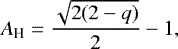
The vertical anisotropy parameter, A_V, is non-zero in all runs, as all have comparable density stratification affecting vertical outflows. Values slightly below one are observed for positive q and for the non-rotating and non-shearing run, while values clearly exceeding unity are obtained for the negative q branch. The simple estimate, Eq. (2), using typical values from observations (as given in Sect. 1), gives vertical anisotropies 3–6 times larger than those obtained from the models. We therefore conclude that, similar to the case of the horizontal anisotropy, the models produce clearly smaller vertical anisotropy than expected. This can be due to the inapplicability of the solenoidality assumption in deriving the estimates, or because of the tendency of turbulence to isotropise itself (e.g. Rotta 1951).

The q vs. − q asymmetry has been reported to be a general property of all the turbulent stresses, including those contributing to the vertical velocity component (e.g. Snellman et al. 2009), which naturally arise through the nonlinear interactions of the three velocity components. Therefore, the most likely explanation of the different values obtained for A_V on the different q branches is this asymmetry. We also note that the rotational and shear-induced anisotropies, even though relatively weak, also interactwith the vertical stratification, and cause additional effects such as the generation of net helicity, discussed in detail in Sect. 3.3.

3.2 Vorticity

The time-evolution of vorticity ω is governed by the following equation, which can be obtained by taking the curl of Eq. (4), $$\text{begin}align*\frac{\partial \overrightarrow{\omega }}{\partial t}\text{ \&}=\underset{\text{induction; omI}}{\underbrace{\overrightarrow{\nabla }\times \left(\overrightarrow{u}\times \overrightarrow{\omega }\right)}}+\underset{\text{baroclinicity; omB}}{\underbrace{\overrightarrow{\nabla }T\times \overrightarrow{\nabla }s}}-\underset{\text{rotation and shear contribution; omRS}}{\underbrace{\overrightarrow{\nabla }\times \left(2\overrightarrow{\text{UpOmega}}\times \overrightarrow{u}+S{u}_x\widehat{\overrightarrow{y}}\right)}}\text{nn \&}-\nu \overrightarrow{\nabla }\times \left(\overrightarrow{\nabla }\times \overrightarrow{\omega }\right)+\nu \overrightarrow{\nabla }\times \overrightarrow{F},\text{nnend}align*$$(17)

where ν is the kinematic viscosity (for simplicity assumed constant, as our interest here is in the other terms), and F_i = 2S_ij∇_j lnρ. The first term on the right-hand side, which we denote $\text{omI}$, is a nonlinear term that can lead to exponential amplification of vorticity, similarly to the induction term $\overrightarrow{\nabla }\times \left(\overrightarrow{u}\times \overrightarrow{B}\right)$ in the magnetic field equation, for example, through the AKA effect. It can be further expanded to the following terms: $$\overrightarrow{\nabla }\times \left(\overrightarrow{u}\times \overrightarrow{\omega }\right)=\underset{\text{stretching;nn omS}}{\underbrace{\left(\overrightarrow{\omega }\cdot \overrightarrow{\nabla }\right)\overrightarrow{u}}}-\underset{\text{advection; omA}}{\underbrace{\left(\overrightarrow{u}\cdot \overrightarrow{\nabla }\right)\overrightarrow{\omega }}}-\underset{\text{compression; omC}}{\underbrace{\overrightarrow{\omega }\left(\overrightarrow{\nabla }\cdot \overrightarrow{u}\right)}}.$$(18)

The first term within this nonlinear term represents the stretching of vortex lines, its contribution to vorticity production being denoted here by $\text{omS}$. The second term is the vortex advection, denoted by $\text{omA}$; this is often subsumed into an advective time derivative on the left-hand side of Eq. (17). The third term is the vortex compression, denoted by $\text{omC}$, which can locally enhance (reduce) vorticity by compression (expansion).

The second term on the right-hand side of Eq. (17) is the baroclinic term, the contribution of which to vorticity generation we denote by $\text{omB}$; this only acts where temperature and entropy gradients are misaligned. The third and fourth terms, collectively denoted by $\text{omRS}$, describe the effect of the imposed rotation and shear, respectively. The final two terms describe the viscous interactions.

Early studies of vorticity generation in the ISM (e.g. Vazquez-Semadeni et al. 1995; Korpi et al. 1999b) give a rather confusing view of the relevance of the processes involved. Vazquez-Semadeni et al. (1995) report on vortex stretching being a powerful sink of vorticity, while Korpi et al. (1999b) show evidence of it being a powerful source; the former further reports on the negligible global role of baroclinicity, while the latter measures significant misalignment of density and temperature gradients and production of vorticity through baroclinicity. The main difference in the aforementioned studies was the type of forcing they used: the former mainly used random forcing with a steep spectrum, while the latter used thermal energy injections modelling supernova forcing. In the former case the maintenance of the vorticity was extremely challenging, while in the latter study the rotational modes clearly dominate over the potential modes, even though the velocity field resulting from SNe in homogeneous and isotropic settings is purely potential. Vazquez-Semadeni et al. (1995) also experimented with wind-type and thermal forcing, and in the latter case vorticity generation was observed, but this was not related to the baroclinicity of the flow.

The problem has attracted relatively little attention until very recent times. Mee & Brandenburg (2006) studied potentially forced flows in an isothermal setup without seed vorticity, and found that viscous interactions arising from the last term in the vorticity equation, which can have non-vanishing curl even for potential flows, were not capable of generating and sustaining vorticity. Del Sordo & Brandenburg (2011) investigated both isothermal and more general thermodynamic systems, but added shear and rotation. They found that neither of these effects can significantly increase the vorticity production in an isothermal system. Only with full thermodynamics included was vorticity production observed. Then the baroclinic term was observed to be significant, especially in the intersections of colliding shock fronts, while the role of the vortex stretching was not considered.

Many studies have so far reported on the existence of large amounts of vorticity and rotational modes in SN-driven flows (e.g. Korpi et al. 1999b; Balsara et al. 2004; Padoan et al. 2016). In the study by Padoan et al. (2016) it is noted that SN driving via thermal energy injection cannot effectively be considered as potential, if SNe go off in an inhomogeneous background density. Such a background is argued to produce baroclinicityat the instant of the energy injection, as the variable density results in accelerations with non-zero curl, even for the purely potential pressure forces. The role of the vortex stretching was not discussed, but the vortex compressionterm was argued to transport energy from rotational to the potential modes. Their analysis was based on inspection of rotational and potential spectra, while neither distribution nor magnitude of the different mechanisms were studied in detail. In the study of Iffrig & Hennebelle (2017) a very similar system was investigated, but with SN forcing modelled by momentum rather than thermal injection, excluding the hot gas produced by SNe (their focus being on colder phases and on structure formation). The compressible modes were observed to dominate near the disk plane, and rotational modes were found only to be important at heights far from the midplane. These results are in apparent contradiction with the other SN forced systems.

Neither the magnitude nor sign of the source terms in Eq. (17) impart any understanding as to their contributionto vortex generation. However, by contracting the equation with the vorticity itself, it becomes evident from the sign (and magnitude) of the product terms whether they are amplifying or diminishing the vorticity (and how strong these effects are). In this study, therefore, we concentrate on monitoring the time evolution of the different terms in the vorticity equation, the relevant results being presented in Table 4, in the form of volume- and time-averaged inner products of vorticity with each source term tracing the time-evolution of its magnitude.

The time-average of the rms vorticity, ω_rms, is only weakly dependent on increasing Co and Sh , indicating that the terms related to rotation and shear are weak. This is confirmed by our monitoring of the term, $\text{omRS}$, related to them, which is several orders of magnitude smaller than the other relevant terms (Table 4). The clearly largest contributor to vorticity evolution is the baroclinic term, $\text{omB}$, which acts as a powerful source of vorticity. The terms contributing to the nonlinear term $\text{omI}$, in contrast, all act as sinks of vorticity. As the baroclinic effect is the strongest, vorticity generation dominates over destruction, and as a net effect a significant rotational component of the flow is generated in all the runs, as discussed earlier. Roughly 65% of the kinetic energy is in the form of rotational energy, agreeing well with the earlier results (Korpi et al. 1999b; Balsara et al. 2004; Padoan et al. 2016).

In Fig. 3 we show the vertical distributions of the horizontally-averaged contributors to vorticity production for Run 1Ωp. The distribution is very similar for the other runs. All quantities show two maxima at about ± 100 pc from the midplane, and a decreasing trend towards the halo region. Closer to the midplane, there is a local minimum. This minimum corresponds to the peak of the SN activity and its associated potential forcing. In particular the cold gas, which is mainly confined near the midplane, accumulates in the shock fronts between interacting SN remnants and is naturally a weak region of vortex generation. In Table 3 the cold phase has systematically weaker absolute and relative vorticity than warm and hot phases. The increase in the proportion of potential energy relative to the squared norm of velocity listed in Table 2 indicates that the high-density, colder medium is more strongly correlated with potential than rotational flow. For |z| > 100 pc away from the midplane, the vertical distribution of baroclinicity and vortex stretching can be described with two exponentials, as shown in Fig. 3 lower panel. Near the midplane, the scale height is roughly 90 pc, coinciding with the type II SNe distribution. At larger heights, the quantities fall off considerably more slowly, the scale height being consistent with 300 pc that corresponds to the type I SNe distribution. The vortex compression is only significant in the vicinity of the midplane, having even smaller scale height than the two other effects.

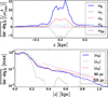Fig. 3 Time-averaged horizontal averages (upper panel) of the inner product of vorticity with vortex sources, ${\overline{\left(\overrightarrow{\omega }\cdot \text{ omX}\right)}}_t$, where $\text{omX}$ are the various terms introduced in Eqs. (17) and (18) due to baroclinicity ($\text{omB}$), vortex stretching ($\text{omS}$), vortex compression ($\text{omC}$), vortex advection ($\text{omA}$), and combined galactic shear and rotation ($\text{omRS}$), for Run 1Ωp (i.e. obtained by contracting Eq. (17) with ω). Lower panel shows the unsigned profiles averaged over upper and lower midplanes, normalised by the maximum of the baroclinicity term at the midplane, together with exponential fits, and the two scale heights used indicated in the legends.

In Figs. 4 and 5 we show the spatial distributions of the most significant contributors to vorticity production with respect to some key system quantities in horizontal and vertical slices of one instantaneous snapshot of the system state. Vorticity is generated throughout the simulation domain (middle panels, green contours), but the regions of strongest vorticity occur inside the clustered SN bubbles with hot and dilute gas. Outside the bubbles, some vorticity is also generated, but on a smaller scale with more patchy distribution. The baroclinicity of the flow is very strong and positive within the SN bubbles, correlating tightly with thevorticity maxima within them. The vortex induction processes act as vorticity sinks particularly in these regions. In the denser and cooler regions the effect of baroclinicity is clearly weaker and even negative, while vortex-induction effects can be stronger, positively contributing to the vorticity generation. It is clear that locally baroclinicity and vortex induction can combine constructively and destructively, but typically the baroclinicity is the more dominant and most positive within the SN bubbles, while the less significant vortex induction acts most positively in the denser interaction regions between expanding SN remnants. The vortex compression is especially well traced by the shock compression regions plotted with the green contour levels on the rightmost panels of Figs. 4 and 5. The vortex stretching shows the most patchy distribution, and is positive only in the regions where density, shown with green contours in the leftmost panel of Figs. 4 and 5, is high.

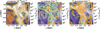Fig. 4 Horizontal slices near the midplane from Run 1Ωp of vorticity contracted with vortex source terms (left to right) baroclinicity, vortex-stretching and vortex-compression. Contours in green (left to right) show gas density, vorticity strength, and flow convergence.

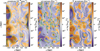Fig. 5 Vertical slices from Run 1Ωp of vorticity contracted with vortex source terms (left to right) baroclinicity, vortex-stretching, and vortex-compression. Contours in green (left to right) show gas density, vorticity strength, and flow convergence.

As evident from Fig. 6, where we show the horizontally-averaged x- and y-components of the vorticity as functions of time and distance from the midplane for Run 1Ωp, there are clear large-scale patterns visible. Such large-scale patterns hint at the existence of z-dependent horizontal mean flows, and therefore deserve more attention. We return to these in Sect. 3.4. We note also the global increase in vorticity around 1010 Myr. SN superbubbles evolve often to occupy a substantial portion of the computational domain, spanning the disk. Sporadically, SNe in or near can rapidly heat these diffuse regions and momentarily accelerate the gas for a large volume filling factor. For the different runs at varying times, such events are also evident in the helicity profiles as displayed later in Fig. 8 and velocity as displayed in Fig. 10.

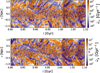Fig. 6 Horizontally-averaged profiles of the horizontal components of vorticity as functions of time, for Run 1Ωp .

3.3 Helicity

The kinetic helicity is an important quantity because the operation ofthe conventional galactic dynamo via the α-effect – describingthe collective inductive action on the mean magnetic field of turbulent motions, under the influence of the Coriolis force – depends upon it. In the case of homogeneous isotropic turbulence, the α-effect can be described with a scalar quantity $$H=\text{vect}u\cdot \overrightarrow{\omega }$$(19)

where τ_c is the correlation time of the turbulence, and ${\overline{(\mathcal{H})}}_{\text{t}}={\overline{(\text{bm}\omega \cdot \text{bm}u)}}_{\text{t}}$ is the time- and horizontally-averaged helicity (e.g. Steenbeck et al. 1966; Rädler 1980). In the more general case of anisotropic turbulence, α is a second-order tensor, its trace ${\Sigma }_{i=1}^3{\alpha }_{ii}$ expected (under simplifying conditions) to be proportional to the helicity (e.g. Rädler 1980). Any inhomogeneity (such as gradients of density or turbulent velocity) together with rotation can be expected to give rise to helicity and therefore to an α-effect, that is, $${\alpha }_{ij}^{\left(\text{UpOmega}\right)}={\alpha }_1^{(\text{UpOmega})}\left(\text{bm}G\cdot \text{bm UpOmega}\right){\delta }_{ij}+{\alpha }_2^{(\text{UpOmega})}\left(G_i{\text{ UpOmega}}_j+G_j{\text{ UpOmega}}_i\right),$$(20)

where G is the gradient of the relevant inhomogeneous quantity and Ω the rotation vector. There are three different vertical inhomogeneities in our system: the gradients in the density and in the intensity of turbulent motions, and the vertical boundaries. Of these three, the density gradient is the strongest, changing by four orders of magnitude, while turbulent intensity only varies by one order of magnitude. For both of these effects, $\text{bm}G\propto \widehat{\text{vect}z}$ on either side of the galactic midplane. In our system, therefore, a positiveα-effect and a negative kinetic helicity can be expected above the midplane, and vice versa below the midplane.

The presence of shear can also lead to the generation of large-scale vorticity; in our system, the imposed azimuthal shear flow, having a linear dependence on x, is prone to give rise to a mean vertical component of vorticity, ${\overline{W}}_z=\partial u_y/\partial x=S$, that is, the large-scale vorticity vector can be written as $\overline{\text{bm}W}=-q\text{bmUpOmega}=(0,0,S)$. It has been proposed, for example, by Rogachevskii & Kleeorin (2003) and Rädler & Stepanov (2006), that such a vortical flow can induce helicity, and as a result also an α-effect of the form $${\alpha }_{ij}^{\left(W\right)}={\alpha }_1^{\left(W\right)}\left(\text{bm}G\cdot \overline{\text{bm}W}\right){\delta }_{ij}+{\alpha }_2^{\left(W\right)}\left(G_i{\overline{W}}_j+G_j{\overline{W}}_i\right).$$(21)

If the shear rate matches the rotation rate in magnitude, but has an opposite sign (which is the case on the positive q-branch runs), one would expect the net helicity to vanish, if the effects act identically through the same inhomogeneity gradient G.

We note that such rotation- and shear-induced-α effects, in agreement with the above-mentioned constructions, have been found from convection simulations with simple, imposed, shear profiles (e.g. by Käpylä et al. 2010). Deviations from the expected profiles, however, were found in the regime of strong shear, which were attributed to the symmetry breaking of the positive vs. negative shear parameter (q) regimes, that had been earlier reported by Snellman et al. (2009) and Korpi et al. (2010). We observe such asymmetry already with a moderate value of |q| = 1, as discussed in detail in Sect. 3.1. Therefore, we might expect that a perfect cancellation of the two effects does not occur in the system studied here either.

The z-profiles of net helicity ${\overline{(\mathcal{H})}}_t$, averaged horizontally and temporally over several turnover times, are plotted in Fig. 7 for our seven different runs. The error bars in the plot depict the standard deviation from the mean over time. Figure 8 shows the time evolution of the corresponding horizontal averages. We also give the volume- and time-averaged net helicities above ($\langle {\mathcal{H}}_N\rangle$) and below ($\langle {\mathcal{H}}_S\rangle$) the disk plane in Table 4. From these tabulated values and plots it is evident that the helicity is a strongly fluctuating quantity, and hardly any net helicity is distinguishable in Run 0Ω0 with no rotation and shear (middle panels), or with weak rotation and shear (Runs 1Ωp and 2Ωp ) on the positive q branch. A significantly clearer signal of net helicity is seen in Run 4Ωp and in all runs on the negative q branch. Strong surges of helicity of varying sign are caused by SN activity originating at larger heights, expanding in the warm and hot phases, on both q branches. The net helicity changes sign such that on the positive q branch the upper (lower) parts of the computational domain are negative (positive), while on the negative q branch the signs are swapped.

Fig. 7 Time- and horizontally-averaged profiles of net helicity, ${\overline{(\mathcal{H})}}_{\text{t}}={\overline{(\text{vect}u\cdot \omega )}}_{\text{t}}$, as a function of height. The error bars show the standard deviation in time, for the relevant horizontal slices. Top row has Runs 4Ωp , 2Ωp , and 1Ωp (left to right), middle 0Ω0, and bottom row 4Ωn, 2Ωn , and 1Ωn (left to right).

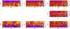Fig. 8 Horizontally-averaged helicity ($\overline{\mathcal{H}}=\overline{\text{vect}u\cdot \omega }$) as a function of time and height. Top row has Runs 4Ωp , 2Ωp , and 1Ωp (left to right), middle 0Ω0, and bottom row 4Ωn, 2Ωn , and 1Ωn (left to right).

Next we will separate the shear-induced net helicity, ${\mathcal{H}}^W$, from the rotation-induced one, ${\mathcal{H}}^{\text{UpOmega}}$. For this, wemake use of the link between ${\overline{(\mathcal{H})}}_t$ and α noted above (whereby ${\mathcal{H}}^{\text{UpOmega}}$ is associated with ${\alpha }_{ij}^{(\text{UpOmega})}$, and ${\mathcal{H}}^W$ with ${\alpha }_{ij}^{(W)}$), and on the parallel constructions Eqs. (20) and (21), to define $$\text{begin}align*{\mathcal{H}}^{+q}\text{\&}=\text{\&}{\mathcal{H}}^{\text{UpOmega}}+{\mathcal{H}}^W,{\mathcal{H}}^{-q}\text{\&}=\text{\&}-{\mathcal{H}}^{\text{UpOmega}}+{\mathcal{H}}^W.\text{nnend}align*$$

The profiles ${\mathcal{H}}^{+q}$ and ${\mathcal{H}}^{-q}$ are the ${\overline{(\mathcal{H})}}_{\text{t}}$ profiles of Runs 1Ωp vs. 1Ωn , 2Ωp vs. 2Ωn , and 4Ωp vs. 4Ωn . The corresponding profiles of ${\mathcal{H}}^{\text{UpOmega}}$ and ${\mathcal{H}}^W$ are obtained from Eqs. (22) and (23), as ${\mathcal{H}}^{\text{UpOmega}}=({\mathcal{H}}^{+q}-{\mathcal{H}}^{-q})/2$ and ${\mathcal{H}}^W=({\mathcal{H}}^{+q}+{\mathcal{H}}^{-q})/2$. We note thathere ${\mathcal{H}}^{\text{UpOmega}}$ and ${\mathcal{H}}^W$ are defined for the positive q branch (i.e. for Ω > 0, S < 0); their signs vary above and below the midplane accordingly. The profiles of ${\mathcal{H}}^{\text{UpOmega}}$ and ${\mathcal{H}}^W$ are shown in Fig. 9.

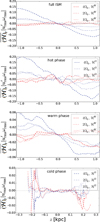Fig. 9 Contributions to the net helicity of rotation (${\mathcal{H}}^{\text{UpOmega}}$, blue lines) and shear (${\mathcal{H}}^W$ red lines) for4Ω0 (dashed), 2Ω0 (dash-dotted) and 1Ω0 (dotted), separated using the runs with opposite rotation using Eqs. (22) and (23).

Fig. 10 Horizontally-averaged flows ${\overline{u}}_x$ (left column), ${\overline{u}}_y$ (centre), ${\overline{u}}_z$ (right) as functions of time and height, for Runs 0Ω0, 1Ωp , 1Ωn , 2Ωp , 2Ωn , 4Ωp , and 4Ωn (from top to bottom).

In the case of |Ω| = |S| = 1, both ${\mathcal{H}}^{\text{UpOmega}}$ and ${\mathcal{H}}^W$ are weak, but show consistently different signs. On the positive q-branch, this will result in the near cancellation of the net helicity, while on the negative q branch (where the opposite sign of ${\mathcal{H}}^{\text{UpOmega}}$ applies) the two effects add up to produce a stronger signal. When rotation and shear are increased, the rotational contribution grows rapidly, while the contribution from shear remains roughly constant or increases only slightly. This results in detectable net helicities also on the positive q branch, while the signal becomes quickly enhanced on the negative q branch.

Separating the net helicities in different phases (see the three lowermost panels of Fig. 9), it is evident that the most significant contributions to both helicity terms come from the hot phase, while the warm phase contributes relatively more significantly to ${\mathcal{H}}^W$. In the cold phase only relatively strong local enhancements occur, and in those regions ${\mathcal{H}}^{\text{UpOmega}}$ and ${\mathcal{H}}^W$ are clearly of different sign. The standard deviations with respect to time behave similarly for both helicity terms; and for both the full ISM and the warm phase, they are of similar magnitude to ${\mathcal{H}}^W$ for each q as a function of z. For the hot gas, in contrast, helicity has high standard deviations near the midplane (between 0.1 and 0.15) for all q; this decreases to below 0.1 for|q| = 1 and 4 for |z| > 0.5 kpc where the helicity for |q| = 4 is at its strongest. So at least for high rotation these trends seem statistically reliable. For the cold phase the standard deviations are strong near the midplane, but small relative to the values of helicity around |z| ≃ 0.2 kpc. The statistics are sparse for the cold phase, but the trend away from the midplane may yet be significant.

It should be noted, however, that these helicity distributions cannot represent the full story for mean-field dynamo action. In a similar system but with magnetic fields included, Evirgen et al. (2017) observe that the mean magnetic field preferentially resides in the warm phase (notwithstanding the helicity distributions noted above); they also note that the presence of a dynamically significant magnetic field actively affects the phase-distribution of the ISM (reducing the volume filling factor of the hot phase), so that subtle nonlinear effects must be anticipated.

3.4 Generation of large-scale flows

As already mentioned when analysing the vorticity generation in the system, large-scale patterns in the horizontal components of the mean vorticity were observed, suggestive of large-scale, z-dependent, horizontal flows. In the system under investigation, the buoyancy force and the momentum of the expanding SN shells can drive systemic flows along the vertical direction of density stratification. We can also expect dynamic changes of such flows, as thevarying SN locations and rate cause local changes around the mean pressure and momentum distribution. Also, our boundary conditions allow both in- and outflows, as locally cooler high-density gas at the boundary will flow in, while hotter less dense gas will flow out. During an epoch of a systematic vertical motion in either direction, matter needs to be replaced (removed) to (from) the region of outflow (inflow) if mass is conserved; therefore, time-dependent horizontal mean flows might also be generated by the mere presence of the vertical outflow. In the following, we investigate whether thehorizontal mean flows are due to such an effect.

In Fig. 10 we plot all components of the horizontally-averaged mean velocities from the seven different runs, as a function of increasing rotation rate (positive or negative). Run 0Ω0 exhibits clear vertical out- and in-flow (upper rightmost panel), that occurs in a semi-regular oscillatory manner. This is due to the disk constantly adjusting its stratification to the changes in the SN activity level. Despite this systematic vertical oscillation, no corresponding structure is seen in the horizontal mean velocity components (upper left and middle panels). When rotation and shear are added (Runs 1Ωp and 1Ωn ; rows two and three), a clear oscillatory pattern also appears in the horizontal components. As the rotation and shear rates are increased, the period of this rather regular oscillation, τ_osc, is decreased (see Table 5). In Runs 2Ωp, 2Ωn , 4Ωp , and 4Ωn (rows four to seven), the horizontal and vertical oscillation periods are already very distinct, and it is clear that they do not relate to each other, but represent two different mechanisms.

To proceed with the analysis, we will write down the equations governing the mean flows in the system. We take a horizontalaverage, denoted with overbars, over the momentum equation and use the Reynolds averaging rules, further setting ∂∕∂x = ∂∕∂y = 0 due to the periodicity in those directions: $$\text{begin}align*\frac{\partial {\overline{u}}_x}{\partial t}\text{ \&}=\text{\&}-{\overline{u}}_z\frac{\partial {\overline{u}}_x}{\partial z}+2{\text{ UpOmega}}_0{\overline{u}}_y-\frac{\partial }{\partial z}\left(\overline{\rho }{Q}_{xz}\right)\frac{\partial {\overline{u}}_y}{\partial t}\text{ \&}=\text{\&}-{\overline{u}}_z\frac{\partial {\overline{u}}_y}{\partial z}-\left(2{\text{ UpOmega}}_0+S\right){\overline{u}}_x-\frac{\partial }{\partial z}\left(\overline{\rho }{Q}_{yz}\right)\frac{\partial {\overline{u}}_z}{\partial t}\text{ \&}=\text{\&}-{\overline{u}}_z\frac{\partial {\overline{u}}_z}{\partial z}-\frac{\partial }{\partial z}\left(\overline{\rho }{Q}_{zz}\right).\text{end}align*$$

Here, the turbulent velocity correlations, that is the Reynolds stresses, are denoted as $Q_{ij}=\overline{{u^{\prime }}_i{u^{\prime }}_j}$. We have assumed that gravity and the pressure gradient balance in the z direction, and we have neglected the contribution of the rate of strain tensor. We note that the Reynolds stress component Q_xy is of great importance for the angular momentum transport in disk systems like the one studied here, and this problem has been under intense investigation for decades (see e.g. Korpi et al. 2010, and references therein). Due to the local periodic system used here, no net horizontal transport is possible, and therefore this Reynolds stress component does not appear in our analysis of mean flows.

Using the mean-field approach (see Rüdiger 1989), it is customary to expand the Reynolds stresses into series containing both non-diffusive and diffusive parts, $$H=\text{vect}u\cdot \overrightarrow{\omega }$$(27)

from which the higher order derivatives can be neglected, under the assumption of scale separation, central to the mean-field approach. In many studies, only the non-diffusive contribution is investigated, but when the mean flows exhibit gradients, which is exactly the case here, both contributions should be properly considered. This would require a method analogous to the test field suite for magnetohydrodynamics (Schrinner et al. 2007). As such a method is currently unavailable, in this paper we rely on simpler, less conclusive, methods.

In our helical, randomly forced system, three potential ways of generating mean flows can be envisioned. One possibility is the Λ-effect (see e.g. Rüdiger 1989), another is the so-called AKA (anisotropic-kinetic-α) effect (see e.g. Frisch et al. 1987; Brandenburg & von Rekowski 2001), and the third is the inhomogeneous helicity effect (Yokoi & Brandenburg 2016). On the other hand, the “vorticity dynamo”, studied in the context of non-helical shear flows, is not possible here since this effect is known to be strongly damped with rotation (see e.g. Elperin et al. 2003), while from Fig. 10 we see that the large-scale flows in the system get stronger and their cycle period shorter when rotation is increased.

The Λ-effect provides a non-diffusive contribution to the Reynolds stresses in anisotropic rotating turbulence, important for angular momentum transport and generation of differential rotation, that can be written in the form $$H=\text{vect}u\cdot \overrightarrow{\omega }$$(28)

In our case, where rotation and the gravity vectors are aligned, there would only be a non-diffusive contribution via the $Q_{xy}^{\Lambda }={\Lambda }_{xyz}{\text{ UpOmega}}_z$ component, which from Eq. (26) would not affect the mean flows generated in the system. Therefore we rule out the Λ-effect as a generator of the mean flows here.

In the study of Yokoi & Brandenburg (2016) it was proposed, and confirmed by direct numerical simulations, that an inhomogeneous turbulent helicity profile is capable of generating large-scale flows even in an incompressible system. The helicity inhomogeneity, however, must be in a direction perpendicular to the rotation axis (see their Eq. (39)), as a result of which a mean flow in the latter direction can be produced. In our system, where the helicity gradient is vertical, coinciding with the rotation axis, this effect cannot explain the emergence of mean flows, although it might contribute to their evolution after they have been generated through some other mechanism. That is, after mean vorticity in the x and y directions (${\overline{W}}_x$ and ${\overline{W}}_y$, respectively) has been generated, we can expect contributions of the type $$\text{begin}align*Q_{xz}^H=\eta {\overline{W}}_x\frac{\partial \overline{\mathcal{H}}}{\partial z},\text{}{Q}_{yz}^H=\eta {\overline{W}}_y\frac{\partial \overline{\mathcal{H}}}{\partial z},\text{nnend}align*$$

where η = C_η (K∕ϵ) (K³∕ϵ²), in terms of the kinetic energy density of the turbulence K, its dissipation rate ϵ, and a closure coefficient C_η that must be optimised for each turbulence model considered. As here we are most interested in explaining the emergence of the horizontal mean flows, we do not pursue this further in the current study.

This leaves only the AKA effect as the original generator of the mean flows. In this mechanism, there is a “kinetic” α-effect proportional to the mean velocities, analogous to the “magnetic” α-effect relating the turbulent electromotive force to the mean magnetic field, producing a non-diffusive contribution to the Reynolds stresses of the form $$Q_{ij}^{\text{non-diff}.}={\alpha }_{ijk}{\overline{u}}_k+\dots$$(31)

While dynamo action through the corresponding term in the induction equation can be obtained in various settings when the flows are helical, the AKA effect requires a special property of the turbulent forcing, namely non-Galilean invariance, which can be achieved through random external forcing. The SN-forced flows considered here are therefore potentially susceptible to this effect.

In von Rekowski et al. (1995), this effect was studied numerically in a disk system resembling the Milky Way, under the assumption of incompressibility. The solutions found were all oscillatory, closely resembling the patterns for the horizontal velocities in Fig. 10. The oscillation frequency increased asa function of the turbulent intensity in the halo gas, although the rotational dependence was not studied.

Pipin et al. (1996) studied the excitation conditions for both the magnetic-α and AKA effects in rotating compressible flows, and found that while the α-effect always grows as a function of rotation, the AKA effect saturates and is actually suppressed in high Coriolis number flows (their Fig. 1). Our Coriolis numbers are small enough to fall on the branch where the AKA effect is still growing as a function of Co, so all the basic findings are favourable for the AKA effect.

On the other hand, Brandenburg & von Rekowski (2001) studied a more idealised system with a tailored forcing function to produce non-Galilean invariant forcing, which also produced kinetic helicity due to the temporal shift employed. Their results suggested that the AKA effect would occur only for low Reynolds number flows, as the energy fraction contained in the large-scale flows driven by the effect decreased as a function of the Reynolds number. According to the trend observed in their study, our setup, with Reynolds numbers of the order of hundreds, should produce at most a very weak AKA effect. Nevertheless, it is constructive to proceed, as helicity is known to have the potential to enhance the instability (e.g. Pipin et al. 1996), and our flow possesses helicity naturally.

Let us now try to assess the possible presence of the AKA effect in oursystem. We first approximate the Reynolds stresses that are capable of driving mean flows, namely Q_xz and Q_yz , using the truncated Taylor series expansion $$Q_{ij}={\alpha }_{ijk}{\overline{u}}_k+{\mathcal{N}}_{ijkl}\frac{\partial {\overline{u}}_k}{\partial x_l},$$(32)

where α_ijk comprises the AKA effect and ${\mathcal{N}}_{ijkl}$ the turbulent viscosity (in the first approximation, although possible inductive effects cannot be completely excluded). These equations contain 2 × 3 unknown coefficients for each of the AKA and viscosity effects (see below). A fit to their dependence on the measurable xy-averaged quantities Q_xz, Q_yz , ū _x , ū _y , ū _z , and the z-derivatives of the mean flows, can be obtained by forming moments with the aforementioned quantities and taking averages over time (which is called the method of moments, see Brandenburg & Sokoloff 2002). After the formation of the moments, we have 2 × 6 equations that can be represented in the following matrix form: $$Q^{(i)}(z)=M(z)C^{(i)}(z),i=x,y,$$(33)

where $$Q^{(i)}=\left(\begin{array}{c}{\langle Q_{iz}{\overline{u}}_x\rangle }_{\text{t}}\\ {\langle Q_{iz}{\overline{u}}_y\rangle }_{\text{t}}\\ {\langle Q_{iz}{\overline{u}}_z\rangle }_{\text{t}}\\ {\langle Q_{iz}{{\overline{u}}^{\prime }}_x\rangle }_{\text{t}}\\ {\langle Q_{iz}{{\overline{u}}^{\prime }}_y\rangle }_{\text{t}}\\ {\langle Q_{iz}{{\overline{u}}^{\prime }}_z\rangle }_{\text{t}}\end{array}\right),C^{(i)}=\left(\begin{array}{c}{\alpha }_{izx}\\ {\alpha }_{izy}\\ {\alpha }_{izz}\\ N_{izxz}\\ {\mathcal{N}}_{izyz}\\ {\mathcal{N}}_{izzz}\end{array}\right),$$(34)

and the matrix M is a 6 × 6 matrix containing all the moments, and is the same for both Eq. (33). The coefficients C⁽ⁱ⁾ can be solved by inverting the matrix M. As the estimation of uncertainties for the coefficients obtained is challenging, we use Run 0Ω0, which has no significant systematic horizontal mean flows, to determine the level of fluctuations in the coefficients. Only if a coefficient shows a clear signal exceeding that obtained for Run 0Ω0 do we consider it significant.

The α coefficients showing clearly significant rms values by this measure are α_xzx, α_yzy, α_xzy, and α_yzx. The profilesof these coefficients as a function of z are plotted for all the runs in Fig. 11; but since α_xzy and α_yzx have similar profiles and values, only α_xyz is plotted. All the coefficients have profiles that are antisymmetric with respect to the midplane, although strong deviations from the general trend are seen. Runs 1Ωp and 2Ωp , in particular, show irregular behaviour between the two half-spaces, and are not always clearly antisymmetric. Most of the irregular behaviour is seen at large heights (|z| ≥±0.5), in which region Run 0Ω0 also shows a spurious systematic signal, while near the midplane only strong fluctuations are visible.

Fig. 11 Profiles of turbulent transport coefficients (obtained from the method of moments) as functions of height. The profile of αyzx (not shown) is similar to that of αxzy .

The profiles of the turbulent viscosity tensor components ${\mathcal{N}}_{xzzz}$ and ${\mathcal{N}}_{yzzz}$, shown for Run 1Ωp in Fig. 11, are positive and symmetric with respect to the midplane. They have peak values comparable to (or greater than) the first order smoothing approximation (FOSA) estimate $H=\text{vect}u\cdot \overrightarrow{\omega }$ over the whole computational volume, using l₀ = 100 pc and 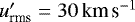$H=\text{vect}u\cdot \overrightarrow{\omega }$. Their rms values, however, are systematically smaller than the FOSA estimate. The other components of the turbulent viscosity tensor are clearly weaker, have both negative and positive values, and show either symmetry or antisymmetry with respect to the midplane. Again, the strongest negative values occur at large heights. Negative values of these tensor components indicate an inductive rather than diffusive character, but given the evidence from the α profiles of spurious signals at large heights, we deem the turbulent viscosity coefficients unreliable for heights more than 0.5 kpc from the midplane. In Table 5, where we list the magnitudes of the turbulent transport coefficients as averages over the vertical coordinate, we therefore only tabulate values for smaller heights, and regard any rms α value smaller than the rotationless and shearless case as insignificant. The level of fluctuations in Run 0Ω0 is close to 2 km s⁻¹, which is rather large in comparison to the FOSA estimate, Eq. 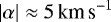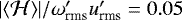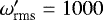(19), which gives $H=\text{vect}u\cdot \overrightarrow{\omega }$, using τ_c = 10⁷ yr, $\text{mathcal{left|left}<H\text{ right}>\text{right|}}/{{\omega }^{\prime }}_{\text{rms}}{u^{\prime }}_{\text{rms}}=0.05$, and ${{\omega }^{\prime }}_{\text{rms}}=1000$ Gyr. This again emphasises that there are large fluctuations in the turbulent transport coefficients for this system.

Now that we have determined estimates for both the non-diffusive and diffusive parts of the turbulent transport coefficients, we can formulate a dimensionless quantity equivalent to the dynamo C_α, describing the magnitude of the inductive effect of turbulence on the magnetic field, following Kitchatinov et al. (1994). Let the parameter Γ describe the magnitude of the AKA effect, H be the disk scale height and ν_t a typical value of the turbulent viscosity; then the AKA number can be defined as $$C_{\text{AKA}}=\frac{\Gamma H}{{\nu }_{\text{t}}}\cdot$$(35)

We list the values of this coefficient in Table 5, based on the maximal AKA tensor component, a disk scale height of 500 pc (descriptive of our runs), and average turbulent viscosity values obtained from the method of moments. We obtain values ranging from roughly 3 to 20. In a one-dimensional mean-field study of galactic disks, assuming incompressibility and the effects of rotation only, Kitchatinov et al. (1994) arrived at an estimate of the critical AKA number being roughly 6. If this critical value was directly applicable to our highly compressible system, including shear, all the runs except 1Ωp would clearly be in the unstable regime. On the other hand, if we consider the turbulent viscosities derived with the method of moments to be inaccurate, and rely on the FOSA estimate instead, then all our C_AKA values would drop below the critical limit. A more definitive study of this issue should involve a thorough analysis of the system via a one-dimensional mean-field model, and should also address the possible role of negative viscosities; we defer this study to a further publication.

3.5 Estimates of turbulent viscosity and the excitation of MRI

In this paper we focus on purely hydrodynamic flows, but in actual galactic disks a dynamically significant magnetic field is present, making them prone to the MRI. Although we cannot directly study here the possible existence/damping of the instability with SN forcing, we can refine the earlier estimates of Korpi et al. (2010) by utilising the more realistic models presented here.

We repeat the analysis of Korpi et al. (2010), where we compared the damping limit derived from the linear stability analysis of the MRI instability, to the corresponding FOSA estimate with values derived from earlier numerical simulations. As discussed in detail in Korpi et al. (2010), the Ohmic diffusion rate can be expressed as $${\text{UpOmega}}_{\text{m}}=\frac{{\eta }_{\text{t}}}{l_0^2}=\frac{\text{ur}}{3l_0},$$(36)

where we either employ the FOSA estimate for the turbulent diffusivity ${\eta }_{\text{t}}=\frac{1}{3}{l}_0\text{ur}$, or use the derived turbulent diffusivity from the method of moments (see Sect. 3.4), assuming η_t = ν_t (implying a turbulent Prandtl number of unity). The damping condition, that is the condition for turbulent diffusion being strong enough to suppress the MRI (see Korpi et al. 2010, for a detailed derivation), is $$H=\text{vect}u\cdot \overrightarrow{\omega }$$(37)

Here, A(q) ≈ 1.4 when q = 1, and Γ_max = qΩ∕2 is the maximum growth rate.

Taking u′rms from Tables1 and 3, and adopting correlation lengths in the range 50 ≤ l₀ ≤ 150 pc (Hollins et al. 2017), we plot our FOSA estimates of the damping condition for the present runs in Fig. 12. We also include the estimates from the AKA-effect analysis, based on the $\text{left}<{\mathcal{N}}_{(x,y)jkl}\text{right}{>}_z$ values presented in Table 5. We note that the correlation lengths are estimated for a run corresponding to our run 1Ωp , but our estimates of the low values of Co and Sh encourage us to proceed.

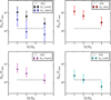Fig. 12 Ohmic diffusion rate Ωm in comparison to the damping condition Ωm ∕Γmax > A(q). Top-left panel shows the FOSA estimate for the total gas the other panels show FOSA estimates for the individual gas phases, as stated in the legends. Each data point is calculated assuming l0 = 100 pc, with the upper and lower uncertainty limits calculated using l0 = 50 pc and l0 = 150 pc, respectively.

The viscosities calculated from the AKA effects are systematically smaller than those from FOSA, and this difference is apparent in the damping conditions. With FOSA estimates, when considering the gas as a whole, the systems stay above the MRI damping condition. Using our AKA viscosities, however, the damping condition is satisfied, throughout the uncertainty range, only for the nominalsolar neighbourhood parameters; higher rotation rates would be prone to the instability for 50 ≤ l₀ ≤ 100 pc. This behaviour as a function of rotation occurs because the maximal MRI growth rate is proportional to the rotation rate, making it increasingly hard, with increasing rotation, to damp the MRI.

As u′rms changes with phase, being lower for cold and higher for hot phases, it is interesting to compute predictions also by phase. With FOSA estimates it appears that, at high rotation rates, the cold phase, and tentatively also the warm phase, could be susceptible to MRI, while the hot phase remains above the damping condition throughout. In contrast, with the AKA estimates, any increase of the rotation rate above the nominal solar neighbourhood parameters would make the majority of the gas in the system susceptible to MRI. However, the MRI damping condition is only indicative, as it arises from a linear stability analysis. Running a full MHD calculation would be required to check for the presence of the instability at higher rotation rates. We note, however, that regardless of the damping for the conditions considered here, MRI may be present outside the star forming regions of galaxies, due to the low SN rates there; and for galaxies with low star formation and high rotation rates, it may even be present in the bulk of the disk.

4 Conclusions

We have investigated the generation of vorticity, net helicity, and mean flows in a simulated ISM extending 1 kpc horizontally and 2 kpc vertically, stirred by SN activity. The key parameters varied were the rotation and shear rates, which were used to change both the vigour of these effects, and also the rotation law of the simulated galaxy. To obtain outwards-decreasing (increasing) angular velocities, we used oppositely directed (aligned) rotation and shear vectors, by changing the direction of the rotation vector. The parameter describing the rotation law, q = −S∕Ω, is positive (negative) in the former (latter) case. The modelling strategy was to keep the magnitude of q fixed while varying the sign of rotation, allowing an attempt to isolate the contributions of shear and rotation to the net helicity generation. One motivation for this study, involving rather unrealistic rotation curves, came from the magnetised counterparts of these simulations, where dynamo action with the nominal solar neighbourhood parameters has been reported either to be possible (Gent et al. 2013b) or not possible (Gressel et al. 2008).

With parameters applicable for the solar neighbourhood of the Milky Way (q = 1), the shear- and rotation-induced contributions to mean helicity are of opposite sign, partially cancelling each other and resulting in a weaker net helicity; whereas on the other branch (q = −1) the two contributions combine, resulting in an enhanced net helicity. This provides one explanation as to why obtaining dynamo action in numerical simulations with solar neighbourhood parameters has been challenging. With higher rotation and shear rates, the almost-complete cancellation of the two effects no longer holds: the net helicity due to rotation is observed to grow faster than that due to shear. The most significant contribution to the net helicity comes from the hot phase of the ISM.

Naturally, only the simulations that correspond to outwards-decreasing angular velocities, in our modelling strategy obtained with positive values of Ω (and q), are relevant for real galaxies; we plan, however, to use the alternative setup further, as it will enable us to study the galactic dynamo process without the additional complication of the MRI. Our analysis on the possibility of MRI excitation shows that within the range of angular velocities explored, the fully magnetic version of the system would only be susceptible to the MRI with the higher rotation rates investigated, and not with the nominal solar neighbourhood parameters. We note, however, that to facilitate dynamo action in systems similar to that investigated here, it is standard procedure to increase the rotation rate by a factor of two (Gent et al. 2013b) or four (Gressel et al. 2008); in that case MRI excitation could be possible, and should be carefully excluded, for example by inverting the rotation law, as done here. Separating the MRI and the dynamo effect due to SNe will not be trivial even then, as is illustrated by our findings on the asymmetry of the turbulent anisotropies on the different q branches. To understand such asymmetries, and the isotropisation of turbulent flows, is an interesting issue on its own, and deserves further attention in a separate, dedicated publication.

One peculiar feature of the supernova-regulated flows is their ability to produce significant amounts of vortical motions, even though such forcing, in a homogeneous background, would be purely divergent, with zero vorticity initially. The decomposition of the flow yields globally orthogonal potential and rotational flows, whose squared norms sum to that of the total velocity field. In this study we measured a dominant rotational contribution with squared norm roughly 65% that of the total velocity across all our runs. Our detailed inspection of the differentvorticity production mechanisms showed that vorticity is efficiently generated within clustered SNe, creating superbubbles, by the baroclinicity of the flow. The vortex induction terms, including the vortex stretching term, were all observed to act as sinks of vorticity in such regions. In the denser, cooler regions where SN shells interact, vortex stretching was also found to act as a source of vorticity, but this mechanism was overwhelmed globally by the baroclinicity within the hotter bubbles. In the earlier work of Korpi et al. (1999b), vortex stretching was found to be much more important as a source. This is probably because the SN distribution in the earlier setup was random in the horizontal plane, in which case superbubble-type clustering could not take place, in contrast to the simulations here. The difficulty of Vazquez-Semadeni et al. (1995) in producing rotational modes even in systems including full thermodynamics is clearly related to the use of random or wind-type forcing in the majority of their runs, which by definition excludes the effect of baroclinicity that naturally arises in systems with pressure gradients in an inhomogeneous environment (Padoan et al. 2016). Also, the results of significantly weaker vorticity production in Iffrig & Hennebelle (2017) have most likely a similar cause: modelling the SN feedback as momentum input is inefficient inproducing baroclinicity. Quite unexpectedly, therefore, the dynamics of SN flows is largely determined at the intermediate scale of forcing, and very strongly depend on the properties of the forcing function. Obviously, including the SN heating as realistically as possible has a decisive rolein such models. If the flow lacks vorticity, then other important effects most likely become suppressed, including small- and large-scale dynamos, for example. These results, therefore, reconcile the old discrepancy of the role of baroclinicity and vortex stretching in SN forced flows.

We also observe the generation of z-dependent horizontal oscillatory mean flows, and seek a cause for this unexpected phenomenon. We rule out the Λ and inhomogeneous helicity effect as the mechanism responsible, and perform a detailed study on the plausibility of the anisotropic-kinetic-α (AKA) effect. Using the method of moments (Brandenburg & Sokoloff 2002), we determine the non-diffusive and diffusive transport coefficients. The latter are consistent although somewhat smaller than the corresponding FOSA estimates. The AKA α is subject to strong fluctuations, but α coefficients significantly larger than those computed from the shearless and rotationless run 0Ω0 are obtained. Also, those diffusion coefficients which should be positive definite are almost entirely positive, thus giving further credibility to this approach. The success of the method of moments in this particular case can be attributed to the presence of oscillatory mean flows that change sign, which are ideal for the fitting method used (in contrast to stationary mean flows). Our estimates of the AKA number, vs. the critical value, consistently predict instability for nearly all the runs that show oscillatory flows, even though the critical values, to which we compare, were determined for a much simpler system. In conclusion, all the evidence considered in this study suggests that the AKA effect should be active in the system.

Acknowledgments

We acknowledge Brigitta von Rekowski, Matthias Rheinhardt, Petri Käpylä, Nishant Singh, Igor Rogachevskii and Nobumitsu Yokoi for many helpful comments and discussions on the manuscript. We also acknowledge the helpful and constructive comments of the reviewer, Anvar Shukurov. This work was carried out under the HPC-EUROPA2 project (project number: 228398), with the support of the European Community – Research Infrastructure Action of the FP7. We gratefully acknowledge the resources and support of the CSC – IT Center for Science Ltd, Finland, where the major part of the code adjustment and all of the production runs were carried out. We also acknowledge the support of the UK MHD Computer Cluster in St. Andrews, Scotland, where some early testing and code development was carried out. Financial support from the Academy of Finland Centre of Excellence ReSoLVE (grant No. 272157) is acknowledged (M.J.K., F.A.G., M.V.). This work has benefitted from travel support by the Max Planck Princeton Center for Plasma physics, and the discussions undertaken during the Princeton 2016 workshop. M.V. thanks the Jenny and Antti Wihuri Foundation for financial support.

References

All Tables

All Figures

	Fig. 1 Representative snapshot from Run 1Ωp with contours on the top, bottom, and back surfaces of the simulation box indicating the ISM temperature (red-yellow), and isosurfaces within the box indicating the gas density (purple-cyan). Streamlines of velocity (green) are plotted through the isosurfaces.
In the text

	Fig. 2 A schematic picture illustrating how the Coriolis and shearing components of the flow influence AH , for positive and negative q (here drawn assuming that ux and uy are positive, with Ω the magnitude of rotation, |Ω|, and for |q| = 1).
In the text

Fig. 3 Time-averaged horizontal averages (upper panel) of the inner product of vorticity with vortex sources, ${\overline{\left(\overrightarrow{\omega }\cdot \text{ omX}\right)}}_t$, where $\text{omX}$ are the various terms introduced in Eqs. (17) and (18) due to baroclinicity ($\text{omB}$), vortex stretching ($\text{omS}$), vortex compression ($\text{omC}$), vortex advection ($\text{omA}$), and combined galactic shear and rotation ($\text{omRS}$), for Run 1Ωp (i.e. obtained by contracting Eq. (17) with ω). Lower panel shows the unsigned profiles averaged over upper and lower midplanes, normalised by the maximum of the baroclinicity term at the midplane, together with exponential fits, and the two scale heights used indicated in the legends.

In the text

	Fig. 4 Horizontal slices near the midplane from Run 1Ωp of vorticity contracted with vortex source terms (left to right) baroclinicity, vortex-stretching and vortex-compression. Contours in green (left to right) show gas density, vorticity strength, and flow convergence.
In the text

	Fig. 5 Vertical slices from Run 1Ωp of vorticity contracted with vortex source terms (left to right) baroclinicity, vortex-stretching, and vortex-compression. Contours in green (left to right) show gas density, vorticity strength, and flow convergence.
In the text

	Fig. 6 Horizontally-averaged profiles of the horizontal components of vorticity as functions of time, for Run 1Ωp .
In the text

	Fig. 7 Time- and horizontally-averaged profiles of net helicity, ${\overline{(\mathcal{H})}}_{\text{t}}={\overline{(\text{vect}u\cdot \omega )}}_{\text{t}}$, as a function of height. The error bars show the standard deviation in time, for the relevant horizontal slices. Top row has Runs 4Ωp , 2Ωp , and 1Ωp (left to right), middle 0Ω0, and bottom row 4Ωn, 2Ωn , and 1Ωn (left to right).
In the text

	Fig. 8 Horizontally-averaged helicity ($\overline{\mathcal{H}}=\overline{\text{vect}u\cdot \omega }$) as a function of time and height. Top row has Runs 4Ωp , 2Ωp , and 1Ωp (left to right), middle 0Ω0, and bottom row 4Ωn, 2Ωn , and 1Ωn (left to right).
In the text

	Fig. 9 Contributions to the net helicity of rotation (${\mathcal{H}}^{\text{UpOmega}}$, blue lines) and shear (${\mathcal{H}}^W$ red lines) for4Ω0 (dashed), 2Ω0 (dash-dotted) and 1Ω0 (dotted), separated using the runs with opposite rotation using Eqs. (22) and (23).
In the text

	Fig. 10 Horizontally-averaged flows ${\overline{u}}_x$ (left column), ${\overline{u}}_y$ (centre), ${\overline{u}}_z$ (right) as functions of time and height, for Runs 0Ω0, 1Ωp , 1Ωn , 2Ωp , 2Ωn , 4Ωp , and 4Ωn (from top to bottom).
In the text

	Fig. 11 Profiles of turbulent transport coefficients (obtained from the method of moments) as functions of height. The profile of αyzx (not shown) is similar to that of αxzy .
In the text

	Fig. 12 Ohmic diffusion rate Ωm in comparison to the damping condition Ωm ∕Γmax > A(q). Top-left panel shows the FOSA estimate for the total gas the other panels show FOSA estimates for the individual gas phases, as stated in the legends. Each data point is calculated assuming l0 = 100 pc, with the upper and lower uncertainty limits calculated using l0 = 50 pc and l0 = 150 pc, respectively.
In the text

References

- Abbott, D. C. 1982, ApJ, 263, 723 [NASA ADS] [CrossRef] [Google Scholar]
- Armstrong, J. W., Cordes, J. M., & Rickett, B. J. 1981, Nature, 291, 561 [NASA ADS] [CrossRef] [Google Scholar]
- Armstrong, J. W., Rickett, B. J., & Spangler, S. R. 1995, ApJ, 443, 209 [NASA ADS] [CrossRef] [Google Scholar]
- Balsara, D. S., Kim, J., Low, M.-M. M., & Matthews, G. J. 2004, ApJ, 617, 339 [NASA ADS] [CrossRef] [Google Scholar]
- Beck, R., Brandenburg, A., Moss, D., Shukurov, A., & Sokoloff, D. 1996, ARA&A, 34, 155 [NASA ADS] [CrossRef] [Google Scholar]
- Bendre, A., Gressel, O., & Elstner, D. 2015, Astron. Nachr., 336, 991 [NASA ADS] [CrossRef] [Google Scholar]
- Berkhuijsen, E. M., Mitra, D., & Mueller, P. 2006, Astron. Nachr., 327, 82 [NASA ADS] [CrossRef] [Google Scholar]
- Brandenburg, A., & Sokoloff, D. 2002, Geophys. Astrophys. Fluid Dyn., 96, 319 [NASA ADS] [CrossRef] [Google Scholar]
- Brandenburg, A., & Subramanian, K. 2005, Phys. Rep., 417, 1 [NASA ADS] [CrossRef] [Google Scholar]
- Brandenburg, A., & von Rekowski B. V. 2001, A&A, 379, 1153 [NASA ADS] [CrossRef] [EDP Sciences] [Google Scholar]
- Brandenburg, A., Nordlund, A., Stein, R. F., & Torkelsson, U. 1995, ApJ, 446, 741 [NASA ADS] [CrossRef] [Google Scholar]
- Chernin, A. D. 1996, Vis. Astron., 40, 257 [NASA ADS] [CrossRef] [Google Scholar]
- de Avillez, M. A., & Breitschwerdt, D. 2005, A&A, 436, 585 [NASA ADS] [CrossRef] [EDP Sciences] [Google Scholar]
- de Avillez, M. A., & Breitschwerdt, D. 2007, ApJ, 665, L35 [NASA ADS] [CrossRef] [Google Scholar]
- Del Sordo, F., & Brandenburg, A. 2011, A&A, 528, A145 [NASA ADS] [CrossRef] [EDP Sciences] [Google Scholar]
- Elperin, T., Kleeorin, N., & Rogachevskii, I. 2003, Phys. Rev. E, 68, 016311 [NASA ADS] [CrossRef] [Google Scholar]
- Evirgen, C. C., Gent, F. A., Shukurov, A., Fletcher, A., & Bushby, P. 2017, MNRAS, 464, L105 [NASA ADS] [CrossRef] [Google Scholar]
- Frisch, U., She, Z. S., & Sulem, P. L. 1987, Physica D Nonlinear Phenomena, 28, 382 [Google Scholar]
- Gaensler, B. M., Madsen, G. J., Chatterjee, S., & Mao, S. A. 2008, PASA, 25, 184 [NASA ADS] [CrossRef] [Google Scholar]
- Gaspari, M., & Churazov, E. 2013, A&A, 559, A78 [NASA ADS] [CrossRef] [EDP Sciences] [Google Scholar]
- Gent, F. A. 2012, Ph.D. Thesis, Newcastle University School of Mathematics and Statistics, http://ethos.bl.uk/OrderDetails.do?uin=uk.bl.ethos.576746 [Google Scholar]
- Gent, F. A., Shukurov, A., Fletcher, A., Sarson, G. R., & Mantere, M. J. 2013a, MNRAS, 432, 1396 [NASA ADS] [CrossRef] [Google Scholar]
- Gent, F. A., Shukurov, A., Sarson, G. R., Fletcher, A., & Mantere, M. J. 2013b, MNRAS, 430, L40 [NASA ADS] [CrossRef] [Google Scholar]
- Gressel, O., Elstner, D., Ziegler, U., & Rüdiger, G. 2008, A&A, 486, L35 [NASA ADS] [CrossRef] [EDP Sciences] [Google Scholar]
- Gressel, O., Elstner, D., & Ziegler, U. 2013, A&A, 560, A93 [NASA ADS] [CrossRef] [EDP Sciences] [Google Scholar]
- Hanasz, M., Otmianowska-Mazur, K., Kowal, G., & Lesch, H. 2009, A&A, 498, 335 [NASA ADS] [CrossRef] [EDP Sciences] [Google Scholar]
- Haverkorn, M. 2015, in Magnetic Fields in Diffuse Media, eds. A. Lazarian, E. M. de Gouveia Dal Pino, & C. Melioli (Berlin: Springer), 483 [Google Scholar]
- Heiles, C., & Troland, T. H. 2003, ApJ, 586, 1067 [NASA ADS] [CrossRef] [Google Scholar]
- Hollins, J. F., Sarson, G. R., Shukurov, A., Fletcher, A., & Gent, F. A. 2017, ApJ, 850, 4 [NASA ADS] [CrossRef] [Google Scholar]
- Iffrig, O., & Hennebelle, P. 2017, A&A, 604, A70 [NASA ADS] [CrossRef] [EDP Sciences] [Google Scholar]
- Käpylä, P. J., Korpi, M. J., & Brandenburg, A. 2010, MNRAS, 402, 1458 [NASA ADS] [CrossRef] [Google Scholar]
- Kitchatinov, L. L., Ruediger, G., & Khomenko, G. 1994, A&A, 287, 320 [NASA ADS] [Google Scholar]
- Korpi, M. J., Brandenburg, A., Shukurov, A., Tuominen, I., & Nordlund, Å. 1999a, ApJ, 514, L99 [NASA ADS] [CrossRef] [Google Scholar]
- Korpi, M. J., Brandenburg, A., Shukurov, A., & Tuominen, I. 1999b, in Interstellar Turbulence, eds. J. Franco, & A. Carraminana, 127 [CrossRef] [Google Scholar]
- Korpi, M. J., Käpylä, P. J., & Väisälä, M. S. 2010, Astron. Nachr., 331, 34 [NASA ADS] [CrossRef] [Google Scholar]
- Krause, F., & Rüdiger, G. 1974, Astron. Nachr., 295, 93 [NASA ADS] [CrossRef] [Google Scholar]
- Kuijken, K., & Gilmore, G. 1989, MNRAS, 239, 605 [NASA ADS] [CrossRef] [Google Scholar]
- Kulkarni, S. R., & Heiles, C. 1988, in Galactic and Extragalactic Radio Astronomy, eds. K. I. Kellermann, & G. L. Verschuur (Berlin, New York: Springer-Verlag), 95 [Google Scholar]
- Levina, G. V., & Burylov, I. A. 2006, Nonlinear Processes in Geophysics, 13, 205 [NASA ADS] [CrossRef] [Google Scholar]
- Mac Low, M.-M., Balsara, D. L., Kim, J., & Avillez, M. A. D. 2005, ApJ, 626, 864 [NASA ADS] [CrossRef] [Google Scholar]
- Mee, A. J., & Brandenburg, A. 2006, MNRAS, 370, 415 [NASA ADS] [Google Scholar]
- Moiseev, S. S., Sagdeev, R. Z., Tur, A. V., Khomenko, G. A., & Shukurov, A. M. 1983, Soviet Physics Doklady, 28, 926 [NASA ADS] [Google Scholar]
- Padoan, P., Pan, L., Haugb∅lle, T., & Nordlund, Å. 2016, ApJ, 822, 11 [NASA ADS] [CrossRef] [Google Scholar]
- Piontek, R. A., & Ostriker, E. 2005, ApJ, 629, 849 [NASA ADS] [CrossRef] [Google Scholar]
- Piontek, R. A., & Ostriker, E. 2007, ApJ, 663, 183 [NASA ADS] [CrossRef] [Google Scholar]
- Pipin, V. V., Rüdiger, G., & Kitchatinov, L. L. 1996, Geophys. Astrophys. Fluid Dyn., 83, 119 [NASA ADS] [CrossRef] [Google Scholar]
- Rädler, K. 1980, Astron. Nachr., 301, 101 [Google Scholar]
- Rädler, K.-H., & Stepanov, R. 2006, Phys. Rev. E, 73, 056311 [NASA ADS] [CrossRef] [Google Scholar]
- Rand, R. J., & Kulkarni, S. R. 1989, ApJ, 343, 760 [NASA ADS] [CrossRef] [Google Scholar]
- Reynolds, R. J. 1977, ApJ, 216, 433 [NASA ADS] [CrossRef] [Google Scholar]
- Reynolds, R. J. 1991, ApJ, 372, L17 [NASA ADS] [CrossRef] [Google Scholar]
- Rogachevskii, I., & Kleeorin, N. 2003, Phys. Rev. E, 68, 036301 [NASA ADS] [CrossRef] [Google Scholar]
- Rosen, A., Bregman, J. N., & Kelson, D. D. 1996, ApJ, 470, 839 [NASA ADS] [CrossRef] [Google Scholar]
- Rotta, J. 1951, Zeitschrift fur Physik, 129, 547 [NASA ADS] [CrossRef] [Google Scholar]
- Rüdiger, G. 1989, Differential rotation and stellar convection, Sun and the solar stars (Berlin: Akademie Verlag) [Google Scholar]
- Ryan Joung, M. K., & Mac Low M.-M. 2006, ApJ, 653, 1266 [NASA ADS] [CrossRef] [Google Scholar]
- Sarazin, C. L., & White, III, R. E., 1987, ApJ, 320, 32 [NASA ADS] [CrossRef] [Google Scholar]
- Schrinner, M., Rädler, K.-H., Schmitt, D., Rheinhardt, M., & Christensen, U. R. 2007, Geophys. Astrophys. Fluid Dyn., 101, 81 endrefcommentnewpage [NASA ADS] [CrossRef] [MathSciNet] [Google Scholar]
- Sellwood, J. A., & Balbus, S. A. 1999, ApJ, 511, 660 [NASA ADS] [CrossRef] [Google Scholar]
- Singh, N. K. 2016, J. Fluid Mech., 798, 696 [NASA ADS] [CrossRef] [Google Scholar]
- Snellman, J. E., Käpylä, P. J., Korpi, M. J., & Liljeström, A. J. 2009, A&A, 505, 955 [NASA ADS] [CrossRef] [EDP Sciences] [Google Scholar]
- Spitzer, L. 1956, Physics of Fully Ionized Gases (New York: Interscience Publishers) [Google Scholar]
- Steenbeck, M., Krause, F., & Rädler, K.-H. 1966, Z. Naturforschung Teil A, 21, 369 [Google Scholar]
- Stepanov, R., Shukurov, A., Fletcher, A., et al. 2014, MNRAS, 437, 2201 [NASA ADS] [CrossRef] [Google Scholar]
- van Weeren, R. J., Brunetti, G., Brüggen, M., et al. 2016, ApJ, 818, 204 [NASA ADS] [CrossRef] [Google Scholar]
- Vazquez-Semadeni, E., Passot, T., & Pouquet, A. 1995, ApJ, 441, 702 [NASA ADS] [CrossRef] [Google Scholar]
- von Rekowski, B., Kitchatinov, L. L., & Rüdiger, G. 1995, in Small-Scale Structures in Three-Dimensional Hydrodynamic and Magnetohydrodynamic Turbulence, eds. M. Meneguzzi, A. Pouquet, & P.-L. Sulem (Berlin: Springer Verlag), Lect. Notes Phys., 462, 355 [CrossRef] [Google Scholar]
- Wolfire, M. G., McKee, C. F., Hollenbach, D., Tielens, A. G. G. M., & Bakes, E. L. O. 1995, ApJ, 443, 152 [Google Scholar]
- Yokoi, N., & Brandenburg, A. 2016, Phys. Rev. E, 93, 033125 [NASA ADS] [CrossRef] [PubMed] [Google Scholar]
Paper I and Gent (2012) have typos (10−16) for as and ad, and are missing z in the first numerator of Eq. (6).
Paper I and Gent (2012) adopt 0.62.
No vertical dependence is imposed in contrast to Paper I, Ryan Joung & Mac Low (2006), Gressel et al. (2008).
All Tables
Parameters and some characteristic quantities computed as volume- and time-averages over the whole computational domain.
Time- and volume-averages of the rotational, , and compressible, , energy per mass as a proportion of the total flow, u2 , obtainedfrom Helmholtz decompositions of u at snapshots every Myr.
Horizontal mean flows and the magnitudes of the turbulent transport coefficients as averages over the vertical coordinate over the range − 0.5 kpc < z < 0.5 kpc.