| Issue |
A&A
Volume 610, February 2018
|
|
|---|---|---|
| Article Number | A51 | |
| Number of page(s) | 23 | |
| Section | Cosmology (including clusters of galaxies) | |
| DOI | https://doi.org/10.1051/0004-6361/201731400 | |
| Published online | 27 February 2018 | |
Replacing dark energy by silent virialisation
1
Toruń Centre for Astronomy, Faculty of Physics, Astronomy and Informatics, Grudziadzka 5, Nicolaus Copernicus University,
ul. Gagarina 11,
87-100
Toruń,
Poland
e-mail: This email address is being protected from spambots. You need JavaScript enabled to view it.
2
Univ Lyon, ENS de Lyon, Univ Lyon1, CNRS, Centre de Recherche Astrophysique de Lyon UMR5574,
69007
Lyon,
France
Received:
19
June
2017
Accepted:
22
October
2017
Abstract
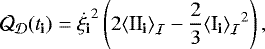
Context. Standard cosmological N-body simulations have background scale factor evolution that is decoupled from non-linear structure formation. Prior to gravitational collapse, kinematical backreaction (QD) justifies this approach in a Newtonian context.
Aims. However, the final stages of a gravitational collapse event are sudden; a globally imposed smooth expansion rate forces at least one expanding region to suddenly and instantaneously decelerate in compensation for the virialisation event. This is relativistically unrealistic. A more conservative hypothesis is to allow non-collapsed domains to continue their volume evolution according to the QD Zel’dovich approximation (QZA). We aim to study the inferred average expansion under this “silent” virialisation hypothesis.
Methods. We set standard (MPGRAFIC) EdS 3-torus (T3) cosmological N-body initial conditions. Using RAMSES, we partitioned the volume into domains and called the DTFE library to estimate the per-domain initial values of the three invariants of the extrinsic curvature tensor that determine the QZA. We integrated the Raychaudhuri equation in each domain using the INHOMOG library, and adopted the stable clustering hypothesis to represent virialisation (VQZA). We spatially averaged to obtain the effective global scale factor. We adopted an early-epoch–normalised EdS reference-model Hubble constant H1EDS = 37.7km s-1 ∕Mpc and an effective Hubble constant Heff,0 = 67.7km s-1 ∕Mpc.
Results. From 2000 simulations at resolution 2563, we find that reaching a unity effective scale factor at 13.8 Gyr (16% above EdS), occurs for an averaging scale of L13.8 = 2.5−0.4+0.1 Mpc∕heff. Relativistically interpreted, this corresponds to strong average negative curvature evolution, with the mean (median) curvature functional ΩRD growing from zero to about 1.5–2 by the present. Over 100 realisations, the virialisation fraction and super-EdS expansion correlate strongly at fixed cosmological time.
Conclusions. Thus, starting from EdS initial conditions and averaging on a typical non-linear structure formation scale, the VQZA dark-energy–free average expansion matches ΛCDM expansion to first order. The software packages used here are free-licensed.
Key words: cosmology: theory / osmological parameters / large-scale structure of Universe / dark energy
© ESO 2018
1 Introduction
Cosmological N-body simulations normally assume that cosmological expansion is gravitationally decoupled from structure formation: scale factor evolution is inserted into the simulation independently of the non-linear structure growth calculated in the simulation. This is a simplification primarily due to the limitations of both analytical and numerical methods of calculation. However, in practice, this decoupling assumption is usually considered to be a corollary of the homogeneity and isotropy assumption underlying the Friedmann–Lemaître–Robertson–Walker (FLRW; Friedmann 1923, 1924; Lemaître 1927, 1931; Robertson 1935) family of cosmological solutions of the Einstein equation, which includes the present standard model of cosmology, the ΛCDM (cosmological-constant–dominated cold dark matter) model. The validity of the decoupling assumption has long been debated (e.g. Ellis & Stoeger 1987; Buchert 2011, and references therein).
Here, our aim is to take into account the role of virialisation and calculate the effective scale factor evolution in an N-body simulation context, guided by general-relativistic constraints defined by scalar averaging (Buchert 2000b, 2001, 2011) that are closely analogous to Newtonian equivalents but are justified relativistically (Buchert et al. 2000, 2013; Buchert & Ostermann 2012). By providing tools for calculating effective background expansion from structure formation itself, we also encourage the community to explore alternatives to the conservative approach adopted in this paper. In Sect. 2, we explain why the standard treatment of virialisation appears to imply, via an externally imposed background expansion rate, a relativistically unrealistic constraint on spatial expansion. Specific calculations to illustrate the argument are given in Sect. 4.
Given that at early redshifts z ≫ 10, the observational distinction between the ΛCDM model and the Einstein-de Sitter (EdS) model (a flat FLRW model with a zero cosmological constant) is very weak, we followed Occam’s razor and adopted an EdS model at early times, setting up standard (MPGRAFIC) cosmological N-body initial conditions. We evolved the initial conditions by a primarily analytical approach – which we refer to here as the kinematical-backreaction ( ) Zel’dovich approximation (QZA). This provides an analytical expression for kinematical backreaction
  evolution in the Newtonian (Buchert et al. 2000) and general-relativistic contexts (Kasai 1995; Morita et al. 1998 in the form Buchert & Ostermann 2012; Buchert et al. 2013; Alles et al. 2015; see also Matarrese & Terranova 1996; Villa et al. 2011), with closely related but differing definitions and meaning.
It has long been accepted observationally that non-linear structure, that is, statistical patterns of overdensities and underdensities with respect to an “average” (mean) density, can be characterised by a length scale of several megaparsecs (Peebles 1974; Peebles & Hauser 1974). If the average expansion history in an initially EdS simulation is distinct from EdS evolution, then it can reasonably be expected that the difference will depend on the choice of length scale corresponding to non-linear structure. Moreover, if the treatment of volume evolution proposed here is a fair approximation of the evolution of the real Universe, then the length scale that yields the appropriate amount of super-EdS scale factor evolution to match a ΛCDM approximation of observational data should be reasonably close to the several-megaparsec scale.
The approach presented here adds detail to previous work in modelling inhomogeneous curvature and expansion (Räsänen 2004; Buchert 2008; Wiegand & Buchert 2010; Buchert & Räsänen 2012) that is constrained by the Raychaudhuri equation and the Hamiltonian constraint (whose spatial averages generalise the Friedmannian expansion and acceleration laws). The recent emergence of average negative scalar curvature in cosmic history (Buchert 2005, 2008; Buchert & Carfora 2008; see also Wiltshire 2007a,b), in which curvature inhomogeneity evolves together with kinematical backreaction (according to a combined conservation law; Buchert 2000b), is found by several of these groups to push the effective scale factor to evolve in a way that potentially mimics “dark energy” on large scales (Roy et al. 2011). Observationally, the non-negligible peculiar expansion rate of voids (Roukema et al. 2013) and the 10%-level environmental dependence of the baryon acoustic oscillation (BAO) peak location (Roukema et al. 2015, 2016) are consistent with a structure formation alternative to dark energy (Roukema et al. 2017). However, precise observational analysis in a more accurate Universe model than the FLRW model requires precise modelling. Specific implementations of emerging negative curvature models have been developed using many different approximations (Räsänen 2006, 2008; Nambu & Tanimoto 2005; Kai et al. 2007; Larena et al. 2009; Chiesa et al. 2014; Wiegand & Buchert 2010; Buchert & Räsänen 2012; Wiltshire 2009; Duley et al. 2013; Nazer & Wiltshire 2015; Roukema et al. 2013; Barbosa et al. 2016; Bolejko & Célérier 2010; Lavinto et al. 2013; see also Sussman et al. 2015; Chirinos Isidro et al. 2017; Bolejko 2017a,b; Krasinski 1981, 1982, 1983; Stichel 2016; Coley 2010; Kašpar & Svítek 2014; Rácz et al. 2017).
There have been very recent attempts to run “fully” relativistic cosmological simulations, which nevertheless require numerical shortcuts and strategies in order to obtain results in reasonable amounts of computing time, and, in some methods, adopt standard flat-space tools such as Fourier transforms. However, these have so far failed to show compatibility with the simpler derivations of emerging average negative curvature models cited above. Two possible reasons for this may be that these codes are too tightly coupled to a background whose average curvature is not allowed to evolve, and they do not appear to take virialisation into account. As explained below in Sect. 2, we adopt the stable clustering hypothesis (Peebles 1980) for virialisation, and the QZA for non-virialised domains, without tightly constraining the average curvature. This approach thus allows the emergence of average negative curvature associated with super-EdS expansion rates.
In the terminology of Adamek et al. (2016a,b), the approach we present here aims to model the growth of what these authors call “homogeneous modes” in their hybrid particle–mesh simulations that aim towards consistency with the Einstein equation. Pure mesh-based cosmological simulation codes aiming at consistency with the Einstein equation include those of Bentivegna & Bruni (2016) and Macpherson et al. (2017) using the free-licensed Einstein Toolkit, as well as those of Giblin et al. (2016a,b). All of these codes assume a T3 spatial section of their Universe model, with the aim being numerical convenience, even though this choice of topology is physically reasonable in terms of the Einstein equation (Aslanyan & Manohar 2012; Ade et al. 2014; Roukema et al. 2014; Aurich 2015; Steiner 2016, and references therein). Our approach only imposes the dynamical constraint of a T3 uniformly flat spatial section in the initial conditions. The mesh-based codes do not yet claim to resolve gravitational collapse (virialisation). The Adamek et al. (2016b) code aims to do this, but is currently tied closely to an FLRW background, and is complementary to the approach presented here (see also Daverio et al. 2017). For approximations related to virialisation and/or gradients of effective pressure in the context of inhomogeneous cosmology, see Buchert (2001), Bolejko & Lasky (2008), Bolejko & Ferreira (2012), and Adamek et al. (2015).
The method adopted here to some degree resembles the Räsänen (2006) approach, in the sense that collapsing and expanding regions are evolved individually, and the Rácz et al. (2017) approach of partitioning N-body realisations into small domains and evolving these in order to generate an effective scale factor evolution. However, both of those approaches assume spherical symmetry to calculate the dynamical evolution of their domains, and neglect spatial continuity by assuming that the kinematical backreaction  is zero, which is only strictly correct in special cases, such as that of spherically symmetric collapse against a spatially flat background (see also Bolejko 2009, regarding Szekeres 1975, models). We do not assume spherical symmetry of domains, we have spatial continuity, and we include the role of
  . Räsänen (2006) does not consider domains whose disjoint union constitutes the global spatial section. Rácz et al. (2017) do consider thedensity of domains whose union gives the full spatial section, but the domains are in reality non-spherical; the authors’ assumption of spherical symmetry is an approximation that assumes kinematical backreaction to be zero. Their domains appear to be non-Lagrangian: shifting of matter across domains does not seem to be taken into account in their Eqs. (3) and (4).
Thus, the method of this paper differs from Räsänen (2006) and Rácz et al. (2017) in that we use generic initial condition realisations over a contiguous spatial section, we calculate kinematical backreaction explicitly and use it in the Raychaudhuri equation for evolving each domain (thus bypassing any need to assume or impose spherical symmetry), and we adopt the stable clustering hypothesis for virialisation. After presentation of definitions and method, the method proposed in this paper is summarised in Definition 1 (Sect. 4.2). Future development of our approach will be to make it free from an assumed reference model, as in the Wiegand & Buchert (2010) volume-partitioning approach or the Wiltshire (2007a,b) biscale partition. The latter divides the spatial section contiguously, though not smoothly, into negatively curved void domains and spatially flat collapsing and virialised structures (“walls”), with a statistical justification for matching walls to the expansion history.
The method is presented in Sect. 3, starting with EdS reference model parameters in Sect. 3.1 and with terminology for the different scales present in N-body simulations in general, and for the method presented here in particular, in Sect. 3.2. The generation of initial conditions on a mesh covering the fundamental domain of the T3 spatial section is presented in Sect. 3.3. This is done using MPGRAFIC (this package and the others used in this work are free-licensed1 software). In Sect. 3.4 we explain how to numerically measure the invariants of what in Newtonian terms is the peculiar velocity gradient tensor. This is only done in the initial conditions for our main model. However, these invariants can also be measured at later time steps for fullN-body calculations.To the degree that the peculiar gradient tensor approximates the (general-relativistic) extrinsic curvature tensor, our approach should not deviate by much from a relativistic approach, even though the initial conditions are defined in Newtonian terms. The library form of the Delaunay Tessellation Field Estimator DTFE, slightly extended by the addition of a small number of functions and corrected for minor bugs, is used to estimate these invariants. The INHOMOG library is introduced in Sect. 3.5. This is used to evolve individual cubical domains using the QZA, each of comoving sidelength  . For convenience and in order to ease the use of this approach in full N-body simulations, this is done using RAMSES-SCALAV, an extension to RAMSES, as a front end to read in the initial conditions and call the DTFE and INHOMOG libraries. In Sect. 3.6 we define how to relate the domain-based average scale factors
  to a global effective scale factor aeff(t).
As a complement to the main model of this work, a method of evolving initially cubical domains  in a full N-body simulation, in which
  is estimated numerically at each major time step instead of evolved using the QZA, is presented in Sect. 3.7. In this case, the Raychaudhuri equation is integrated by following the Lagrangian volume defined by the particles of each initial domain and again calculating an effective global expansion rate aeff (t). This approach again uses RAMSES-SCALAV as a front end for reading in initial conditions, and DTFE as the library for calculating the peculiar velocity gradient invariants. The INHOMOG library is not used in this case.
Since the estimation of  is crucial to this work, the accuracy of the DTFE numerical estimation of the peculiar velocity gradient invariants (and thus
  ) is presented in Sect. 5.1. The main results of this work, the comparison of effective scale factor evolution to EdS evolution and ΛCDM evolution, are presented in Sect. 5.2. In Sect. 5.3, the close relation between virialisation and super-EdS global effective expansion is shown. In Sect. 5.4, we briefly compare our main results with those of calculating
  numerically in our N-body comparison method. The relation between Newtonian and relativistic reasoning is discussed again in the light of these results, qualitatively presenting a perfect fluid effective model of virialisation, in Sect. 6. A summary and conclusions are given in Sect. 7. We set the spacetime unit conversion constant (Taylor & Wheeler 1992) c := 1 unless otherwise specified. Appendix A provides a computer algebra script for confirming the equivalence of expressions for invariants of the peculiar velocity gradient tensor (Eq. (11)). Appendix B provides the correct expression for the variance of the third invariant, which is wrong in Eqs. (C20)–(C22) of Buchert et al. (2000).
2 Virialisation versus spatial expansion
Although the aim here, as in several related projects, is general-relativistic cosmology simulations, it is useful to consider Newtonian reasoning. However, defining a mathematically solid Newtonian cosmological model is not easy. Buchert & Ehlers (1997) showed that a T3 Newtonian cosmological model defined in terms of a dust fluid and gravitational potential, which avoids the divergent infinite sum problem in the pointwise two-point attraction approach, can provide a self-consistent solution (see also Ehlers & Buchert 1997; Ellis & Gibbons 2014 for a recent review and an interesting family of solutions; and recent reminders in Kaiser 2017; Buchert 2018). In this case, if  evolution inlocal domains is calculated within the constraints of the same (expanding) T3 “absolute” space, then the global scale factor evolution of an initially EdS model retains EdS behaviour (proportionality to t2∕3), even when scale factor evolution is calculated in the local domains
  using
using  and averaged. In terms of kinematical backreaction, the global
  (see Sect. 3.4.2). (Eq. 61) of Buchert et al. 2000, is incorrect; the middle element of the double equation has to be omitted to make the equation correct.) However, this justification for exact EdS global expansion is only valid until gravitational collapse and virialisation (or more generally, shell-crossing). Before discussing virialisation, let us first consider the QZA, that is, the algebraic expression for evaluating
  time evolution as presented in Buchert et al. (2000) and Buchert et al. (2013) in the spirit of the Zel’dovich approximation (Zel’dovich 1970).
The QZA evolution of the kinematical backreaction  has the same algebraic structure in the Newtonian (Buchert et al. 2000, Eq. (42); Buchert et al. 2013, Eq. (57); NZA) and relativistic (Buchert et al. 2013, Eq. (50)) cases, but with differing spatial definitions and interpretations (Buchert et al. 2013, IV.A); we cite this expression in Eqs. (30), (31). This expression for
  evolution is exact for some particular cases in the Newtonian context (Buchert et al. 2000, III.D, III.E). In the relativistic context, it is exact for plane symmetric collapse (Buchert et al. 2013, Eq. (75)) and provides exact solutions for certain cases of spherically symmetric collapse (Lemaître 1933; Tolman 1934; Bondi 1947; LTB) models (Buchert et al. 2013, V.B.1). The QZA requires knowing the growth function for linear perturbations in a reference model (in our case, the EdS reference model), and of the initial invariants of the extrinsic curvature tensor. Here, we estimate the latter using the Newtonian peculiar velocity gradients, generated for a standard T3 cosmological N-body simulation. The initial invariants in non-global domains should collectively satisfy a partitioning formula (Buchert & Carfora 2008, Sect. 3.2; Wiegand & Buchert 2010, Eqs. (16), (17)) that yields globally zero mean invariants due to the T3 constraint; see Sect. 3.4.2 for details.
How are virialisation, Newtonian and relativistic reasoning related? The assumptions of the Newtonian collisionless, compressible fluid approach for exact spherically symmetric collapse, interpreted strictly, imply collapse to a singularity in a finite time. A Lagrangian model is easier to relate to a relativistic model than an Eulerian model in the sense that the Lagrangian approach ties matter and space together directly. However, in this idealised case of spherical collapse, a positive Lagrangian volume drops suddenly to zero at the final moment of collapse. In other words, the validity of the approach is limited to times before gravitational collapse events occur. More generically, the assumptions fail when shell crossing first occurs. In N-body simulations or with physical particles, the usual way to avoid these Newtonian singularities is to adopt a hybrid fluid-particle model: the fluid model allows the model to be defined globally as shown by Buchert & Ehlers (1997, or approximated regionally in an adaptive mesh refinement method), while virialisation of a set of particles is expected (and modelled) to occur instead of singularity formation. At a small enough scale, baryon pressure also opposes gravitational collapse. Disregarding baryon pressure, overdensities in a T3 N-body simulation cannot be strictly spherically symmetric because they are composed of particles; and they cannot evolve in an exact spherically symmetric way because the global spatial section is T3. Moreover, Gaussian initial conditions will generically lead to at least moderately anisotropic collapse. Finally, excessively high two-particle close-encounter accelerations are avoided by a small-length-scale softening parameter. Thus, the limitations of the Newtonian fluid approach are dealt with in N-body simulations by considering singularity formation to be unrealistic (unless a simulation is detailed enough to include active galactic nucleus formation and star formation through to supermassive and stellar black hole formation).
This avoidance of singularity formation is generally modelled without any overt compensation in volume evolution at the global T3 volume evolution level. Below we argue that in the standard approach (whether analytical or N-body), there is, in fact, hidden compensation in volume evolution at the global level.
In this work, we are not interested in modelling the details of virialisation. What is relevant for a relativistic interpretation is whether or not compensation between volume loss and gain in collapsing and expanding (respectively) Lagrangian domains is included in the model. It is clear that, when interpreting observations in terms of FLRW models, the virialisation of high-mass collapsed objects correlates closely with the cosmologically recent appearance of a non-negligible value of the dark energy parameter (ΩΛ). This observational clue is quantified in Roukema et al. (2013). Relativistically, the assumption of no sudden compensation between virialising and expanding domains can be described as a “silent virialisation” approximation (following Matarrese et al. 1994b,a for the somewhat different “silent Universe” approximation; see also Ellis & Tsagas 2002; Bolejko 2017b).
In Sect. 4, we present a two-domain partition of the T3 volume that illustrates our claim that the standard approach of passing from pre- to post-virialisation is relativistically unrealistic. In Sect. 4.1, we define the biscale partitions and study volume evolution prior to the collapse and virialisation event. In Sect. 4.2, we present the dilemma between choosing the standard approach versus using the QZA for the expanding domain and the stable clustering approximation for virialised domains (presented in more detail for our main multi-domain partition modelling in Sect. 3.5.6). We thus define the Virialisation  Zel’dovich Approximation.
3 Method
3.1 EdS reference model extrapolated from early epochs
The use of an Einstein–de Sitter (EdS) reference model at early times (that we previously called a “background” EdS model; Roukema et al. 2013, 2017) or on large spatial scales in inhomogeneous cosmological models that aim to be more accurate than the FLRW model risks leading to confusion when referring to “the” Hubble constant, since several different values compete for this name. Here, as in Roukema et al. (2017), we set up the EdS reference model in terms of a reference-model scale factor aEdS and a reference-model expansion rate HEdS given by
 (1)
(1)
where 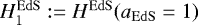 . This EdS model is intended to approximately fit early epochs. In order to derive an observationally realistic value of
  , an effective scale factor aeff which is nearly identical to the reference model scale factor at early times, that is, aeff ≈ aEdS for small t, is adopted. This is done by normalising to aeff = 1 at the present time
  , where the Planck Surveyor (Table 4, sixth data column, Ade et al. 2016) parametrisation of the ΛCDM model is used as a proxy for cosmological observations. As explained in Roukema et al. (2017), this requires that we adopt an early-epoch–normalised EdS–reference-model Hubble constant
  km s-1 ∕Mpc (Rácz et al. 2017 adopt this value too) and an effective Hubble constant – the limiting value that should be observed in the local few hundred Mpc according to an FLRW fit of the data – Heff,0 = 67.74km s-1 ∕Mpc.
3.2 Scales
A standard T3 N-body simulation has three built-in length scales:
- (i)
Lbox – the side length of the fundamental domain, often called the box size,
- (iv)
LN – the mean interparticle separation along one of the three fundamental directions between “adjacent” particles among a set of N1∕3 particles sorted along that axis, where the simulation contains N particles; that is, LN := Lbox∕N1∕3, and
- (v)
Lsoft – the softening length of Newtonian two-point instantaneous attraction; in the case of RAMSES (Sect. 3.7), this can be considered to be the maximum level of resolution for calculating the Newtonian gravitational potential in an adaptively defined cell, Lsoft := 2−levelmaxLbox.
We insert two additional scales between Lbox and LN (we order the definitions from (i) to (v) to monotonically match length scales). Non-linear structure formation has characteristic scales (Peebles 1974; Peebles & Hauser 1974), so as in earlier work, we need to set a scale at which we estimate the kinematical backreaction  and apply the scalar averaged evolution equations (Sect. 3.5). Since
  is an average of the peculiar velocity gradient tensor invariants, the latter should be estimated at a smaller scale. However, to reduce the Poisson noise effects of using a finite number of particles, the scale at which these invariants are estimated (Sect. 3.4) should be greater than LN. Thus, our intermediate scales are
- (ii)
 – the scalar averaging initial domain size in comoving units (Sect. 3.5), and
 - (iii)
LDTFE – the DTFE mesh size (Sect. 3.4).
We correspondingly define
 (2)
(2)
Using this terminology, numerical scalar-averaging modelling of cosmological expansion requires, in general,
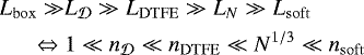 (3)
(3)
for an N-particle simulation, where the validity of the minimal ratios in this multiple inequality needs to be studied both numerically and analytically. Setting the first three ratios of these values to 8 or 16 would require N = 5123 or 40963, respectively. Given these heavy requirements in computer resources, we limit this initial study to numerical exploration of the modest value N = 2563. For our main calculations, in which the QZA uses only the initial values of the invariants of the peculiar velocity gradient (in a Newtonian interpretation), nsoft is irrelevant. For the N-body comparison, we use N = 1283 and set nsoft∕(N1∕3) = 32.
3.3 Initial conditions
We use the free-licensed (GNU General Public License, version 2 or later; GPL-2+) package MPGRAFIC-0.3.10 (Bertschinger 2001; Prunet et al. 2008)2 to generate cosmological initial conditions for an EdS model, with 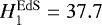 km s-1 ∕Mpc – which, in the absence of structure formation, would give a unity scale factor (for the reference model) at the unrealistically late foliation time of 17.3 Gyr (see Eq. (1)).
The comoving fundamental domain size Lbox (see Sect. 3.2) needs to be expressed in units of ![Mathematical equation: $\mathrm{Mpc}/[H_1^{\mathrm{EdS}}/(100~\mathrm{km\,s}^{-1}\!/\mathrm{Mpc})]$](/articles/aa/full_html/2018/02/aa31400-17/aa31400-17-eq36.png) , since the simulation starts with the EdS reference model. However, in order for length scales to be interpretable in terms of standard descriptions of low-redshift observations, it is more useful to choose Lbox based on a given low-redshift length scale LDTFE, so as above, we adopt the Ade et al. (2016) estimate of Heff,0 = 67.74km s-1 ∕Mpc. Thus, we have
, since the simulation starts with the EdS reference model. However, in order for length scales to be interpretable in terms of standard descriptions of low-redshift observations, it is more useful to choose Lbox based on a given low-redshift length scale LDTFE, so as above, we adopt the Ade et al. (2016) estimate of Heff,0 = 67.74km s-1 ∕Mpc. Thus, we have
![Mathematical equation: \begin{align*} \frac{L_{\mathrm{box}}}{\mathrm{Mpc}/[H_1^{\mathrm{EdS}}/(100~\mathrm{km\,s}^{-1}\!/\mathrm{Mpc})]} &= \frac{L_{\mathrm{box}}}{\mathrm{Mpc/}h_{\mathrm{eff}}} \frac{H_1^{\mathrm{EdS}}}{H_{\mathrm{eff},0}} \nonumber \\ &= \frac{L_{\mathrm{box}}}{L_{\mathrm{DTFE}}} \frac{L_{\mathrm{DTFE}}}{\mathrm{Mpc/}h_{\mathrm{eff}}} \frac{H_1^{\mathrm{EdS}}}{H_{\mathrm{eff},0}}, \end{align*}](/articles/aa/full_html/2018/02/aa31400-17/aa31400-17-eq37.png) (4)
(4)
where heff := Heff,0∕100 km s-1 ∕Mpc.
We match the Ade et al. (2016) power spectrum normalisation of 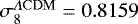 to our EdS reference model. We evolve the effective Planck-parametrised ΛCDM model backwards to z = 1000, that is, to t = 547 Myr, and then forwards using our EdS model, obtaining σ8 = 1.0395 when aEdS = 1, which we use for MPGRAFIC initial conditions.
The value of LN is set in MPGRAFIC, and later read in automatically by RAMSES.
3.4 Estimating “velocity gradient” invariants
In order to model what from a general-relativistic point of view is the extrinsic curvature tensor, we numerically estimate what in Newtonian terms is the peculiar velocity gradient tensor. That is, we make the standard assumption that world lines of particles can have their time derivatives separated into “peculiar velocities” and a refence model expansion aEdS(t).
Delaunay and Voronoi tessellation are two methods that Bernardeau & van de Weygaert (1996) argued provide close to optimal tracing of the (Newtonian) peculiar velocity field. Here, we use the former, as implemented in the Delaunay Tessellation Field Estimator (DTFE)3 which is a free-licensed code that has been found to be highly competitive in comparison with other codes that aim to extract peculiar velocity fields from cosmological N-body simulations (Schaap & van de Weygaert 2000; van de Weygaert & Schaap 2009; Cautun & van de Weygaert 2011; Kennel 2004), with good tracing of the details of the cosmic web of virialised structure (Aragón-Calvo et al. 2010a,b; Sousbie 2011; Park et al. 2013; Pranav et al. 2017). DTFE uses the free-licensed library CGAL (Computational Geometry Algorithms Library4) to make Delaunay tessellations.
A Delaunay tessellation of an N-body simulation snapshot is a division of the T3 volume into tetrahedra using the particles’ positions, in such a way that none of the particles lies inside the circum-2-sphere of any of the tetrahedra. Given one such tetrahedron with vertices k = 0, 1, 2, 3 and simulation peculiar velocity vectors at these vertices  , i = 1, 2, 3, a linear interpolation of the peculiar velocity gradient
  relates velocity component changes from the 0th to the kth vertex for k≠0
 (5)
(5)
for the usualEinstein summation notation over corresponding upper/lower indices and a comma in the subscript to indicate a partial derivative. If the matrix  is invertible (which, in numerical practice, should almost always be the case), the velocity gradient can be estimated as
 (6)
(6)
We use DTFE to carry out this linear interpolation using DTFE “method 1”. This consists of Monte Carlo sampling with a quasi-random spatial distribution within a Delaunay tetrahedron, giving interpolated values that accumulate in cubical cells of a regular grid of  cells within the simulation box, yielding an averaged interpolated estimate of
  in each DTFE grid cell.
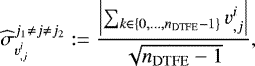
3.4.1 S1-based estimates of velocity gradient uncertainties
We introduce a method of estimating the DTFE grid estimates of  that does not seem to have been used previously. This new method is based on the numerical estimate of the integral of
  over any closed straight loop S1 passing through the nDTFE points
  in an
in an  cubical DTFE grid of velocity gradient estimates in a time slice of a simulation, where k ∈ {0, …, nDTFE − 1}, and xj1, xj2 are two fixed values in thej1th, j2 th directions, respectively,with j1 ≠ j ≠ j2. Analytically,
 (7)
(7)
should hold by the second fundamental theorem of calculus (Stokes’ theorem) if  is continuous and real-valued. Provided that we allow the usual S-shaped peculiar velocity profiles across filaments and virialised objects, this should be satisfied by a standard interpretation of the information numerically represented by the simulation particles.
Numerically, we make the assumption that the numerical uncertainty  is Gaussian and identically and independently distributed at each of the DTFE grid points along a given S1 loop. This is obviously an oversimplification. Collapsing or expanding structures on scales greater than LDTFE could reasonably lead to correlations in numerical errors in the estimates of
  across close pairs of DTFE grid points, and tensor invariants of
  have represent symmetries that may exacerbate these correlations. It is also quite realistic for the per-grid-point errors to be non-gaussian. Nevertheless, this order of magnitude estimate of the error depends on very few assumptions, and provides a consistency check that can be interpreted in terms of expected failures of these minimal assumptions.
Thus, we introduce
 (8)
(8)
where we use nDTFE − 1 to increase the error estimate slightly at low nDTFE, and the absolute value becomes irrelevant when this formula is used in Eq. (9) below. There is no constraint i = j: the velocity components’derivatives need to correspond to the direction of integration, but the velocity components themselves do not need to. This provides  estimates for a fixed direction j. We define the rms (root mean square) of these
  error estimates of the ith component summed in the jth direction:
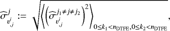 (9)
(9)
where k1, k2 label the grid positions in the j1th, j2 th directions, respectively. We introduce this into DTFE with the function ESTIMATESIGMAGRADIENTONEDIREC. For propagating these uncertainties to estimates in uncertainties in the scalar invariants of  (Sect. 3.4.2), we estimate the rms over the diagonal and off-diagonal components of
  separately:
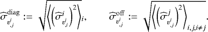 (10)
(10)
These two error estimators summarise and simplify the uncertainty information from the S1 constraint from all velocity gradient components in all three orthogonal directions (of the simulation interpreted as a Newtonian simulation) over the whole fundamental domain. The motivation for separating diagonal from off-diagonal components is that in a physically realistic simulation, this might help to separate different types of error.
3.4.2 S1 and T3-based uncertainties in I and II
In flat space, the tensor invariants of the peculiar velocity gradient can be written (Buchert 1994; Ehlers & Buchert 1997; see Appendix A for a derivation)
![Mathematical equation: \begin{align*} {\mathrm{I}}(v^i_{,j}) :=&\; \mathrm{tr}(v^i_{,j}) = v^i_{,i} = \nabla \cdot {\boldsymbol{v}} \nonumber \\ {\mathrm{II}}(v^i_{,j}) :=&\; \tfrac{1}{2} \left\{ \left[\mathrm{tr} \left(v^i_{,j}\right) \right]^2 - \mathrm{tr} \left[ \left(v^i_{,j}\right)^2 \right] \right\} \nonumber \\ =&\; \tfrac{1}{2}\left((v^i_{,i})^2 - v^i_{,j}\, v^j_{,i}\right) \nonumber \\ =&\; \tfrac{1}{2}\nabla\cdot \Big({\boldsymbol{v}} (\nabla\cdot{\boldsymbol{v}}) - ({\boldsymbol{v}}\cdot\nabla){\boldsymbol{v}} \Big) \nonumber \\ {\mathrm{III}}(v^i_{,j}) :=&\; \mathrm{det} (v^i_{,j}) \nonumber \\ =&\; \tfrac{1}{3} v^i_{,j}\, v^j_{,k}\, v^k_{,i} - \tfrac{1}{2} v^i_{,i} \, (v^i_{,j}\, v^j_{,i}) + \tfrac{1}{6} (v^i_{,i})^3 \nonumber \\ =&\; \tfrac{1}{3} \nabla\cdot\Bigg\{ \tfrac{1}{2} \; \left[ \nabla\cdot \Big( {\boldsymbol{v}}(\nabla\cdot{\boldsymbol{v}}) - ({\boldsymbol{v}}\cdot\nabla){\boldsymbol{v}} \Big) \; \right] \; {\boldsymbol{v}} \nonumber \\ &\;- \left[ \; \Big({\boldsymbol{v}}(\nabla\cdot{\boldsymbol{v}}) - ({\boldsymbol{v}}\cdot\nabla){\boldsymbol{v}}\Big) \cdot\nabla\right] \;{\boldsymbol{v}} \Bigg\},\end{align*}](/articles/aa/full_html/2018/02/aa31400-17/aa31400-17-eq62.png) (11)
(11)
where v := (v0, v1, v2). Thus, all three invariants can be expressed as divergences, so that Stokes’ theorem again applies, this time over the full T3. Again, sums of I, II, or III over the full simulation volume should analytically be zero, but numerically should indicate the level of numerical noise. However, assuming that the DTFE grid over the full box gives statistically independent and identically distributed errors is likely to be a worse approximation than assuming this within any S1 straight loop. Nevertheless, global means of the invariants and of kinematical backreaction (see Eq. (16) below) can be checked for consistency with zero based on the S1 method of error estimation.
Again assuming statistically independent gaussian errors and using Eqs. (11) and (16), we obtain an S1 -based uncertainty for  , and
, and  of
of
![Mathematical equation: \begin{align*} \widehat{\sigma}_{{\left\langle {{{\mathrm{I}}}} \right\rangle_{{\cal D}}}} &= \sqrt{3} \,{\widehat{\sigma}_{{v}^i_{,j}}^{\mathrm{diag}}} \nonumber \\ \widehat{\sigma}_{{\left\langle {{{\mathrm{II}}}} \right\rangle_{{\cal D}}}} &= \sqrt{ {\left\langle {2 \, \left(\widehat{\sigma}_{{v}^i_{,j}}^{\mathrm{diag}}\, {v}^i_{,i}\right)^2 + \left[\widehat{\sigma}_{{v}^i_{,j}}^{\mathrm{off}}\, {v}^i_{,j} (1-\delta^j_i)\right]^2} \right\rangle}_{{\vec x}} } \nonumber \\ \widehat{\sigma}_{{{\cal Q}}_{{\cal D}}} &= \sqrt{ 4 \, {\widehat{\sigma}_{{\left\langle {{{\mathrm{II}}}} \right\rangle_{{\cal D}}}}}^2 + \frac{16}{9} \, {\widehat{\sigma}_{{\left\langle {{{\mathrm{I}}}} \right\rangle_{{\cal D}}}}}^2 {{\left\langle {{v}^i_{,i}} \right\rangle}_{{\vec x}}}^2 },\end{align*}](/articles/aa/full_html/2018/02/aa31400-17/aa31400-17-eq65.png) (12)
(12)
where x represents all  DTFE grid points and
  is the usual Kronecker delta.
To test DTFE’s numerical accuracy in estimating velocity field gradients, we define analytical velocity fields
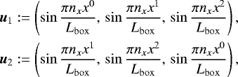 (13)
(13)
for which I and II are straightforward to calculate analytically; the only non-zero gradient components are aligned with the sinusoidal directions in u 1, and orthogonal to them in u2 (giving I(u2) = 0 = II(u2)). We study the two following questions:
- (i)
What is the signal-to-noise ratio (S∕N) of the rms of u1 or u 2, where the signal is defined by Eq. (13) and the noise σmeas is the rms of the difference between the analytical expression for I or II and the numerical estimate?
- (ii)
What is the ratio of σmeas to the rms error predicted by the S1-based error estimators indicated above (Eqs. (8)–(10), (12))?
The results of these calculations using TEST_VGRAD_DTFE.CPP in DTFE are presented in Sect. 5.1.
3.5  Zel’dovich approximation (QZA)
Here we present our method of integrating the averaged Raychaudhuri evolution at the  scale, used in our method (i), that we implement in the INHOMOG free-licensed (GPL-2+) library5. Averaging of
  within the full volume, that is, at the box scale Lbox, is discussed below in Sect. 3.6. For the reader’s convenience, we make this subsection slightly more general than is needed for the specific method adopted here: we include the case of a non-zero cosmological constant Λ.
3.5.1 Scalar averaging equations
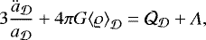
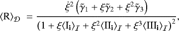
The averaged Raychaudhuri equation in the relativistic case (Buchert et al. 2013, Eq. (9)) is:
 (14)
(14)
where  is defined in the usual way (Buchert et al. 2013, Eqs. (2), (3)), we write the per-domain scale factor and volume evolution in terms of their initial (i) values
  ,
,  is the mass in the domain
  , and the averaged Hamiltonian constraint (Buchert et al. 2013, Eq. (10)) is:
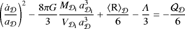 (15)
(15)
(Buchert 2000a,b, 2001), where the kinematical backreaction is defined in terms of the invariants of the extrinsic curvature tensor, approximated in terms of the invariants of the velocity gradient tensor on a domain  :
:
 (16)
(16)
For a more physically motivated definition in the Newtonian case, see Buchert et al. (2000, II.B., Eq. (5), Appendix A).
We use DTFE to numerically estimate the initial values of these invariants on a regular cubical mesh of  comoving positions in the EdS reference model. Thus, each domain
  (again a cubical cell) contains
 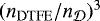 estimates of I and II. We average these to obtain
  and
and  . As stated above (Eq. (3)), it should be preferable to have
  .
.
We only consider the Λ = 0 (dark-energy–free) case here, since Occam’s razor favours first calculating a DE-free model with expansion generated consistently with structure formation, which is the main theme of this paper. Non-flat FLRW backgrounds are more difficult to model correctly, since Fourier analysis is invalid in these cases; the power spectrum needs to be expressed in terms of an orthonormal basis for a constant non-zero curvature 3-manifold of the appropriate topology.
3.5.2 Initial invariants and other initial conditions
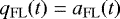
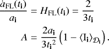
The INHOMOG software allows the reference model scale factor a(t) to be normalised at unity either at the initial time or at the present, setting (cf. Buchert et al. 2000, C.1 last paragraph)
 (17)
(17)
so that
 (18)
(18)
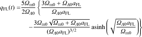
where the subscript “FL” indicates the FLRW reference model. In this paper, the reference model is the EdS model described in Sect. 3.1, and aFL(ti) is set as described in Sect. 3.3. In Buchert et al. (2013), the reference model is termed a background.
Buchert et al. (2000) internally alternates between defining the invariants of the extrinsic cuvature tensor and the (normalised and zeroed) growth function ξ ((34) below) to have a time dimension ([I] = T−1, [II] = T−2, [III] = T−3, [ξ] = T, where [x] denotes the dimension of x and T is the time dimension) or to be dimensionless. Buchert et al. (2013) uses the dimensional definitions throughout, except in Sect. VI.A. Here we adopt the dimensionless definitions. This requires the replacements
 (19)
(19)
everywhere in the text of Buchert et al. (2013) except for Section VI.A, where the growing mode qFL (t) is given in Eqs. (35) or (36). In many formulae, the replacements cancel so that the published formulae are unaffected by this change of convention.
Numerical evaluation of these invariants for the RZA version of the QZA formalism developed in Buchert et al. (2000); Buchert & Ostermann (2012); Buchert et al. (2013) requires using a power spectrum in the reference model, so the spatial section of the reference model must be  or T3 (some other flat FLRW spatial sections also allow Fourier analysis). Here we adopt a standard
  power spectrum (Eisenstein & Hu 1998).
Buchert et al. (2013) VI.A gives the initial conditions for  (for brevity we drop the “RZA” pre-superscript), following from (A3) and (49) in Buchert et al. (2000), where here we use the dimensionless definition of the growth rate ξ and the invariants, and a bold i subscript toindicate that the invariants are calculated at the initial time on the domain
  in Lagrangian coordinates (
 ),
),
 (20)
(20)
An alternative choice would be to use the Hamiltonian constraint (15) and assume that the initial epoch is early enough that turnaround has not yet been reached,  , in order to select the positive square root for
  , yielding

where we postpone expresssions for  and
and  to (37) and (38) below.
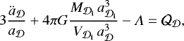
3.5.3 Evolution equation
Writing the per-domain density  , Eq. (14) becomes
 (23)
(23)
and with Buchert et al. (2013, Eq. (92)) (with a dimensionless definition of ξ and the invariants) can be expressed as
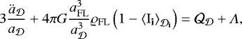 (24)
(24)
and thus, using (18),
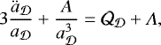 (25)
(25)
where the constant A is defined
 (26)
(26)
with HFL := ȧFL∕aFL and  the usual FLRW matter density parameter. For the EdS reference model we have
 (27)
(27)
This allows (22) to be rewritten
 (28)
(28)
and the Hamiltonian evolution equation becomes
 (29)
(29)
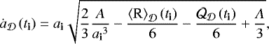
Typical collapsing solutions start with  , the positivesquare root. Finding the first local minimum of
  in the positive square root case yields an estimate of the turnaround epoch tturn (when
  drops to zero), enabling a switch to the negative square root for an initial approximate solution that continues through to collapse. Iterative improvement of the estimates of tturn and
  yields improved accuracy.
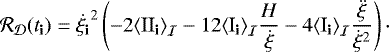
3.5.4 Auxiliary equations
To numerically solve Eq. (15) would require estimating the evolution of both the kinematical backreaction  and the mean curvature
  . The kinematical backreaction is given by Buchert et al. (2013, Eq. (50)) (or its Newtonian equivalent):
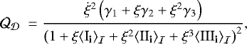 (30)
(30)
where
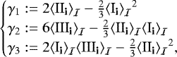 (31)
(31)
and the subscript  indicates that a fully relativistic calculation would integrate the curved, Riemannian volume even at thisearly time when perturbations are weak, and the dimensionless growth rate ξ is given in Eq. (34). The mean curvature is given by Buchert et al. (2013, Eqs. (13), (54)) for the flat FLRW background case:
 (32)
(32)
where
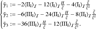 (33)
(33)
As detailed below in Sect. 3.5.5, we bypass the direct dependence on  by integrating Eq. (25) instead. Evaluation of these expressions requires the growth rate ξ(t), for which we use the dimensionless form of Buchert et al. (2013, Eq. (32)),
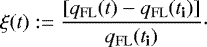 (34)
(34)
For the EdS reference model, the growing mode is
 (35)
(35)
(for example, Chapter 15, Weinberg 1972; Eq. (21), Bildhauer et al. 1992). For completeness, the growing mode for low-density flat FLRW backgrounds (such as ΛCDM) with present density parameter Ωm0 < 1 and ΩΛ0 := 1 − Ωm0 is:
 (36)
(36)
(Bildhauer et al. 1992, Eq. (21)).
Since ξi = 0 by definition (see (34)), the initial backreaction terms needed in (28) follow from (30)–(33):
 (37)
(37)
and
 (38)
(38)
For EdS, we have 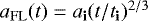 , so from (17) and (27) we have
 (39)
(39)
The standard FLRW expressions can be used for the low-density flat background case.
3.5.5 Numerical strategy
The Raychaudhuri Eq. (25) is a second-order ordinary differential equation (ODE), which can be reduced to two first-order equations
![Mathematical equation: \begin{eqnarray*} \dot{a}_{{\cal D}} &=& y \nonumber \\ \dot{y} &=& \frac{1}{3} \left[(\CQ_{{\cal D}}+\Lambda) a_{{\cal D}} - \frac{A}{a_{{\cal D}}^2} \right],\end{eqnarray*}](/articles/aa/full_html/2018/02/aa31400-17/aa31400-17-eq128.png) (40)
(40)
where  is defined toclarify the numerical strategy. This pair of first-order equations can be solved numerically by calculating
  from (30) and (31) and the initial values of the invariants
  ,
,  , and
, and  , and setting the scale factor initial conditions from Eq. (20) and the constant A from Eqs. (27) or (39), and the growth function from Eq. (35). In principle, as in Ostrowski et al. (in prep.), typical values of
  ,
,  , and
, and  , could be evaluated under the assumption of Gaussianity of the initial invariants, using Eqs. (C5), (C14) and (C18) of Buchert et al. (2000) and the corrected equivalent of Eqs. (C20)–(C22) of Buchert et al. (2000), which we provide here in Eq. (B.2) in Appendix B, since it has not been published previously. However, in this work, we estimate
  ,
,  , and
, and  from the initial conditions generated by MPGRAFIC, which only assumes Gaussianity of the density fluctuations. Thus, the distributions of the second and third invariants of the peculiar velocity gradients are not constrained to be Gaussian.
Numerical solvers for ODEs often require Jacobians. In the case of Eq. (40), these are
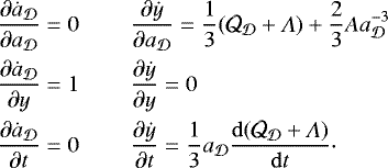 (41)
(41)
We solve these equations using the embedded Runge–Kutta–Fehlberg (4, 5) method of the GNU SCIENTIFIC LIBRARY (GSL) routine GSL_ODEIV_STEP_RKF45.
The averaged density parameters then follow from (18) and (19) in Buchert et al. (2013),
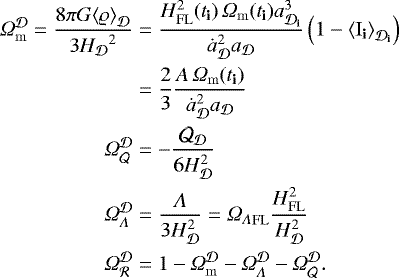 (42)
(42)
3.5.6 Virialisation
After turnaround of a given domain  , that is, when
  becomes negative, we continue integration towards numerical collapse (
 ) at foliation time tcoll. The initial solution
  is used as an approximation that is improved iteratively. We assume virialisation – we set
 (43)
(43)
where 18π2 is the usual EdS stable clustering (Peebles 1980) virialisation overdensity (Lacey & Cole 1993, Eq. (A16)).For completeness, the INHOMOG package provides the corresponding value for the flat-Λ case if that is chosen, using the fitting formula of Bryan & Norman (1998, Eq. (6)) to Eke et al. (1996)’s calculation.
As motivated below in Sect. 4, we do not introduce any behaviour in other domains that compensates for virialisation events. Indeed, it is not obvious how such compensating volume evolution could reasonably be approximated, apart from imposing the reference model expansion rate and abandoning the aim of estimating structure-generated effective expansion.
3.6 Regional versus global averaging
As in Räsänen (2006, 3.1) and Rácz et al. (2017), we cubically average the domain-wise scale factors,
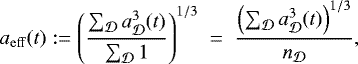 (44)
(44)
where the volumes of collapsed domains are bound below by their virialisation volumes at the time of collapse, as defined in Eq. (43). Although this represents volume averaging at the global level, virialisation is not represented in  , so unless
  is chosen large enough for no virialisation events to occur, Eq. (14) is expected to fail at the global level, since the single fluid stream assumption fails at virialisation. Thus, aeff (t) = aEdS(t) is not expected in the presence of virialisation. See Sect. 6.1 for more discussion of this point.
3.7 RAMSES front end and N-body measurement of 
The two main classes of faster simulation techniques are tree codes and particle-mesh (PM) based methods (e.g., Bagla 2005; Dehnen & Read 2011). In this work, we provide a patch to the adaptive mesh refinement (AMR) RAMSES code6 (Teyssier 2002; Guillet & Teyssier 2011), available under CeCILL (GNU GPL compatible) as Fortran 90 code, that we tentatively refer to as RAMSES-SCALAV7 This serves as a front end to read in the initial conditions files (Sect. 3.3) and call the DTFE and INHOMOG libraries to estimate the per-domain initial invariants  ,
,  , and
, and  , and to carry outVQZA evolution and volume averaging as described in Sects. 3.5 and 3.6.
In an initial exploration of more numerical approaches, the RAMSES-SCALAV front end also allows  to be calculated numerically from the invariants at each major time step using Eq. (16) instead of using the QZA analytical calculation of (30) and (31), which is based on the initial values of the invariants and the growth rate of the reference model. We then integrate Eq. (25), again rewriting it in the form of Eq. (40). In this case, we integrate using the classical (non-adaptive) Runge–Kutta (fourth-order) algorithm. As in Sect. 3.6, we average the domain-level scale factors
  to obtain aeff using Eq. (44). For any given domain
  , we store the list of particles initially present in
  , and at time t we calculate
  and
and  by weighting I and II by the volume element dμi of the ith particle. All parameters Ii, II i and d μi are calculated as (Euclidean) linear interpolations of the I, II and 1∕ρ values of the eight neighbouring DTFE cells surrounding the particle. The global normalisation between d μi and 1∕ρi is arbitrary.
Since we do not change the list of particles in a domain between time steps, the domain shape, which we can conceptually imagine as the union of Voronoi tessellation tetrahedra surrounding the particles, is unlikely to remain cubical. It is likely to become irregular and disconnected. The domain at late times will contain holes that exclude particles that have entered from neighbouring domains, and will include small islands of space around particles that have escaped the main body of the domain. In principle, this is not a problem, since Eq. (25) is based on Riemannian (or Lebesgue in the case of a global T3 domain) integration, which is additive.
By default, a RAMSES cosmological simulation runs like a typical N-body simulation, with the reference model expansion inserted at each time step from a pre-calculated model, decoupled from structure formation. For future work, our RAMSES-SCALAV front end makes it easy to adopt a more consistent approach, that is, to use the cubically averaged aeff(t) (Eq. (44)) when calculating the Newtonian gravitational potential that is used for inferring accelerations of particles. In the present work, we limit calculations to those using the reference model EdS scale factor evolution, in order to compare with the VQZA approach.
4 VQZA super-EdS expansion: biscale partition
Räsänen (2006) proposed that the volume average of expanding and contracting domains defined against an FLRW reference model may evolve differently from, and in particular, at later times, evolve faster than the background. As stated in Sect. 2, prior to virialisation, this claim fails in a strictly Newtonian T3 case for contiguous space: the kinematical backreaction  in the expanding and contracting domains is a non-linear effect that compensates for what otherwise appears to be dynamical asymmetry in non-linear evolution of initially small density perturbations. This was established in Buchert & Ehlers (1997).
4.1 Newtonian conservation of EdS expansion prior to virialisation
We illustrate this here by dividing a T3 volume of an EdS model into exactly two domains  and
and  of initially equal volume: T
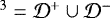 ;
; 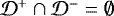 ;
;  . We set
  to be the expanding domain and
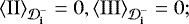
  the contracting domain. Thanks to Stokes’ theorem, the global (Newtonian) averages of the three invariants of the peculiar velocity gradient (approximating what in the relativistic case is the peculiar expansion tensor; see III.B.1 in Buchert et al. 2013), where the invariants are given in Sect. 3.4.2, are each zero on this compact spatial 3-manifold. With volume partitioning (see Wiegand & Buchert 2010, Eqs. (16), (17)) and our choice to give the two domains initially equal volumes, we have per-domain average initial invariants related by
 (45)
(45)
Using Eqs. (30), (31), (34), and (35), the QZA on this biscale volume split should provide approximate confirmation that the EdS scale factor evolution is conserved during a Newtonian pre-virialisation period in cases in which the QZA is approximate, and exact (within numerical accuracy) confirmation in cases in which it is exact.
We consider several subcases – a class that includes planar collapse:
 (46)
(46)
a class that includes spherically symmetric expansion or collapse:
 (47)
(47)
and cases where either  or
or  is set to zero and the non-zero invariants are set to values that give terms in Eqs. (30) and (31) of roughly similar orders of magnitude. Specific values are indicated in the caption of Fig. 1.
The planar collapse class of solutions (Buchert et al. 2000, III.D) constitute an exact solution family, which is clearly supported numerically in Fig. 1 prior to the collapse of the collapsing domain at about 6.2 Gyr. Prior to 6.2 Gyr, the global super-EdS scale factor ratio is unity to within a precision of |1 − aeff(t)∕aEdS| < 2.3 × 10⁻⁵, where aeff is defined in Eq. (44). In other words, prior to virialisation, the QZA in the planar class of solutions is fully consistent with the Newtonian T3 cosmology that is normally used to calculate structure formation in the flat FLRW models (EdS and ΛCDM).
The spherical symmetric class of solutions is also exact (Buchert et al. 2000, III.E), with γ1 = γ2 = γ3 = 0. However, if Eq. (47) is satisfied so that the expanding domain  is a member of this class, then Eq. (45) prevents the contracting domain from satisfying Eq. (47) (with
  replaced by
  ), since the squared second invariant is necessarily positive in both cases. Thus, a small deviation from global EdS evolution is visible in Fig. 1: the global super-EdS scale factor ratio is close to unity but drops a few percent below unity just prior to the collapse at 4.3 Gyr. The other two cases show similar levels of deviation from an exact global EdS expansion just prior to collapse of the collapsing domain.
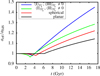 |
Fig. 1 Pre- and post-virialisation EdS-normalised scale factor evolution aeff∕aEdS for a biscale partition evolved using the VQZA as motivated in Sect. 2 and defined in Sect. 4. From bottom to top at t ≳ 7 Gyr, the arbitrarily chosen dimensionless values of the average initial invariants (at initial scale factor |


4.2 Aftervirialisation: the VQZA
In Fig. 1, the global scale factor evolution follows from assuming the stable clustering hypothesis (Eq. (43)) for the collapsed domain and by assuming that the expanding domain continues its expansion as given in the QZA in Eqs. (30), (31), (34), and (35). This conservative assumption motivates the following definition.
Definition 1.
Virialisation  Zel’dovich approximation (VQZA):
- (i)
divide a large volume to be studied into contiguous domains
 ;
; - (ii)
evolve the scale factor
 in each domain according to the Raychaudhuri equation (Eqs. (25), (26)), where the kinematical backreaction
  is approximated by the
  Zel’dovich approximation (QZA) (Eqs. (11), (30), (31)), unless gravitational collapse and virialisation (iii) occur at some time tcoll;
 - (iii)
if virialisation (Sect. 3.5.6) occurs in a domain
 , QZA evolution ceases at t = tcoll
and the stable clustering approximation (Eq. (43) in the EdS case) for
, QZA evolution ceases at t = tcoll
and the stable clustering approximation (Eq. (43) in the EdS case) for  is adopted for t ≥ tcoll
for the domain
is adopted for t ≥ tcoll
for the domain  ;
; - (iv)
the global scale factor evolution is estimated by cubical averaging of the per-domain scale factors
 (Eq. (44)).
Is this model Newtonian or relativistic? Our aim is to model spatial expansion in a close approximation to general-relativistic behaviour. As discussed above, a fully Newtonian cosmology is difficult to define. The Buchert & Ehlers (1997) fluid model justification of T3 Newtonian cosmology does not apply past shell-crossing. When one domain collapses and the others continue expanding, should there be a sudden compensation in the behaviour of the expanding domain(s) in response to the virialisation of the collapsed domain? We hypothesise that this particular feedback effect would not occur in a relativistic model. In other words, we hypothesise silent virialisation: that the details of collapse have a negligible effect at large distances from the collapsing domain (Matarrese et al. 1994b,a; Ellis & Tsagas 2002; Bolejko 2017b). In this sense, the VQZA is a relativistic approximation. It is not exactly relativistic. For example, the sum of rest masses is conserved via the constants A used in per domain Raychaudhuri integration (Eqs. (25), (26)); peculiar velocities of the order of 10−2.5 would imply that the system mass (in the Minkowski spacetime sense) should be about 10−5 higher than the sum of the rest masses. In work closely analogous to the present paper, Bolejko (2017b,c) uses a silent Universe family of cosmological solutions of the Einstein equation based on four scalar quantities (density, expansion rate, shear and Weyl curvature). That model numerically evolves an ensemble of worldlines starting with ΛCDM initial conditions, making similar assumptions to those of the VQZA: stable clustering and silent virialisation. The emergence of strong negative mean curvature is inferred in those works.
The dynamical difference between the VQZA and the standard approach is also shown in Fig. 2 in the biscale case. This figure shows the evolution of the expanding domain  in the VQZA (+ symbols) compared with evolution that follows the standard (implicit) dynamical assumption made about expanding domains in cosmological N-body simulations and typical analytical calculations (solid curves). The latter is defined by
 (48)
(48)
where the factor of two represents division of the spatial section into two domains. The expanding domain has smooth VQZA behaviour independently of the collapse event. In contrast to the smooth volume evolution under the VQZA, the standard model implicitly requires the expanding domain(s) to be suddenly pulled more strongly by the virialised object once collapse and virialisation have finished, in order to preserve a globally EdS expansion rate:  has to suddenly become less positive or more negative when
  very rapidlyswitches from a strong negative value to zero.
Interpreted relativistically, the expanding domain prior to collapse corresponds to negatively curved space that is below the critical density. This is shown in Fig. 3 for the same biscale examples. The curvature functional isgiven in Eq. (42) in the VQZA case. In the EdS constraint case, we again interpret  relativistically (an EdS model is intended as a relativistic, not Newtonian, model), using the partitioning formula, Eq. (10) of Wiegand & Buchert (2010) applied to a globally flat spatial section,
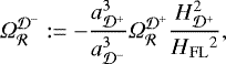 (49)
(49)
where the  factor converts between globally normalised and per-domain normalised definitions of Ω. Following collapse, the stable clustering assumption gives
  , and both domains are interpreted as flat. Thus, in the EdS constraint case, the expanding domain in the biscale case needs to suddenly switch from smooth
  growth to
  . Interpreted from a Newtonian point of view, this sudden switch is allowed; here, we hypothesise that it is relativistically inaccurate.
Ironically, it is the standard model that assumes a form of feedback (backreaction) in this situation; by not adopting this virialisation-induced feedback, the VQZA is more conservative than the standard approach.
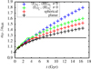 |
Fig. 2 Expanding-domain scale factor evolution |

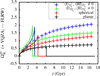 |
Fig. 3 Mean curvature functional |


5 Results
In studying the question of whether dark energy can be replaced by a non-linear structure formation scale at a first level of approximation, we treat the ΛCDM model as an observational proxy, as in Roukema et al. (2017). In principle, given the microlensed Galactic Bulge star likely upper age limit of 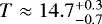 Gyr (Bensby et al. 2013; Roukema et al. 2017) and EdS CMB fits indicating an age of the Universe slightly higher than this (Blanchard et al. 2003; Hunt & Sarkar 2007; Nadathur & Sarkar 2011), it could reasonably argued that we should consider the structure formation scale that yields an effective scale factor aeff that reaches unity just a little earlier than t = 15 Gyr, rather than the ΛCDM current age of the Universe estimate of t0 = 13.80 Gyr. Nevertheless, it is premature to make detailed observational tests using the VQZA approach, so in this work we consider the ΛCDM proxy estimate of the age of the Universe as a reasonable first-order approximation.
5.1 Uncertainties in peculiar velocity gradient invariants I and II
Measurement of  is crucial to calculating volume evolution, so we first consider numerical uncertainties. Application of the error estimation methods described inSects. 3.4.1 and 3.4.2 to the test functions (Eq. (13)) are illustrated in Figs. 4–6, using the DTFE version indicated in Table 1.
Figure 4 shows values mostly greater than unity. In other words, given that we know the true test-function velocity field u1 (Eq. (13)), numerical DTFE estimates of the first and second tensor invariants of the peculiar velocity gradient tensor typically have errors of smaller amplitude than the signal. This is consistent with the claims in the literature regarding DTFE’s accuracy (Schaap & van de Weygaert 2000; van de Weygaert & Schaap 2009; Cautun & van de Weygaert 2011).
The nx = 64, nDTFE = 256 points for both I and II (upper and lower plots, respectively) are for DTFE sampling at a higher resolution than the N = 1283 particle resolution. That is, one full sinusoidal wavelength of u1 in one direction is sampled by about two particles, and DTFE estimates the velocity gradient at four grid points along this direction. To obtain any reasonable velocity gradient in this situation would obviously push the extremes of the available information content, so obtaining S∕N ~ 1, as shown in both panels of the figure, is clearly reasonable.
However, the error estimates in Fig. 4 are based on prior knowledge of the true velocity field, which, in general, is not the case. The S1-based error estimation method introduced in Sect. 3.4.1 bypasses this requirement. Figure 5shows that this new method appears to be viable, in the sense that the ratios of rms measured noise to rms predicted noise are within at most two orders of magnitude of unity. The assumptions of statistical independence and Gaussianity used in the derivation of Eq. (8) are unlikely to be fully satisfied, so better agreement between modelled and measured noise would be surprising. Structures sized just twice that of the particle resolution (nx = 64 = N∕2, asterisks) tend to give the worst (highest) ratios. Most of the ratios worsen when the DTFE resolution is higher than the particle resolution (nDTFE = 2N). These behaviours are reasonable.
The measured-to-predicted noise ratios for the second invariant II (u 2) (Fig. 5, lower panel, lower curves with + and × symbols) mostly are lower than unity. That is, the measured errors are lower than that given by Eq. (8). This is presumably related to the fact that II(u2) = 0, and possibly also to symmetries in sampling this function which cancel each other very effectively, so that the assumption of statistically independent distributions overestimates the noise level.
Global (T3) application of Stokes’ theorem gives consistent error propagation results to those for the S1 -based estimates, to within a few orders of magnitude. Figure 6 shows that  (global first invariant) errors are bounded above by the S1-based errors with Gaussian error propagation. In contrast,
  errors are only bounded above by the S1-based errors for large structures (nx = 1 or 8). Structures whose wavelength is twice that of the particle resolution (nx = 64 = N∕2, asterisks) numerically fail the analytically required
  test at many nDTFE resolutions. The equivalent plot for
  is not displayed, because the low amplitude of
  estimates and Eq. (16) make the
  contribution negligible, giving a plot visually identical to that for
  , but raised by a factor of two.

 |
Fig. 4 Signal-to-noise ratios S∕N of I (above) and II (below) representing the ratio of rms signal to rms numerical noise σmeas, for analytical model u1 (which has non-zero invariants) in Eq. (13), sampled by realisations of N = 1283 particles drawn from a uniform spatial random distribution for 8 ≤ nDTFE ≤ 64. The signal is negligibly small for nDTFE = 16, 128 for nx = 8, 64, respectively,since the test functions are sinusoidal and in phase with the box. |
 |
Fig. 5 As in Fig. 4, ratio of measured noise σmeas to rms error predicted by S1-based error estimators for I (above) and II (below), for both models u1 and u 2. These ratiosare within two orders of magnitude of unity in both cases. |
 |
Fig. 6 As in Fig. 5, measured global |


5.2 VQZA super-EdS expansion
Figure 7 shows effective scale factors for VQZA simulations with  and an MPGRAFIC grid of N = 2563 particles, with
  increasing within any of the three panels as labelled, and
  increasing from two in the top panel to eight in the bottom panel. (See Table 1 for software versions.) The scale factor growth is very close to EdSfor
  and
and  . This is reasonable, because typical overdensities on these scales do not have time to collapse by the present.
On smaller averaging scales  , silent virialisation (the VQZA, Definition 1, Sect. 1) starts to play a role in volume expansion. This can be seen in Fig. 7, where the scale factor growth is stronger as
  decreases. The ΛCDM proxy scale factor evolution (× symbols) mostly lies between the
  and 4 Mpc∕heff curves. In other words, these curves provide the required super-EdS expansion required to reach a unity effective scale factor aeff (t) by t = 13.8 Gyr.
Figure 7 also indicates that the preferred  scale for providing sufficient super-EdS expansion is only weakly sensitive to the choice of Lbox, LDTFE, and LN. The spacing between the curves in any individual panel is not uniform: this is very likely a sign of cosmic variance: the Lbox sizes here are small. The box size Lbox can be increased further, but at the expense of leaving only small ratios
  and LDTFE∕LN. Figure 8 shows that
  is still favoured in this case.
By running a large number of these simulations, we can estimate L13.8, the value of  which gives aeff(13.8 Gyr) = 1. This is done here as follows. For a set of five simulations with different
  values, as in one of the panels of Fig. 7, estimate
  by a spline of t against aeff (t) for each simulation. Least-squares fit a quadratic to
  and solve
  Gyr to obtain
  . We find that for
  (as in Fig. 7, middle panel), 100 sets of 5 simulations yield an averaging scale of L13.8 = 2.51 ± 0.22 Mpc∕heff. This is the scale at which aeff (t) reaches a unity scale factor at 13.8 Gyr, which is 16% above aEdS(13.8 Gyr). The error estimate is the standard deviation of the 100 estimates. This error estimate represents the effect of cosmic variance for 4 Mpc∕heff ≤ Lbox ≤ 64 Mpc∕heff.
Corresponding values for smaller and bigger box sizes,  (Fig. 7, top panel) and
  (Fig. 7, bottom panel), are L13.8 = 2.14 ± 0.26 Mpc∕heff and L13.8 = 2.59 ± 0.25 Mpc∕heff, respectively, for 100 sets of 5 simulations of N = 2563 particles in each case. Thus, the uncertainty in changing the box size and resolution parameters is of about the same magnitude as the uncertainty associated with cosmic variance, and about ten times the standard error in the mean of L13.8 for any fixed set of size and resolution parameters. We summarise these by writing the (dominating) systematic error and taking the median of the three sets of calculations (
 , as in Fig. 7, middle panel, for one quintuple of realisations):
  .
.
We alsocarried out 100 sets of five simulations on still bigger box scales (as in Fig. 8), at the risk of greater numerical error due to the small factors between the shorter length scales ( ). This set of simulations gives a much more precise estimate: L13.8 = 2.56 ± 0.01 Mpc∕heff, most likely because of the reduced cosmic variance. However, since there is a greater risk of numerical error, this estimate is not likely to be more accurate (the resolution-related systematic error is likely to be higher). Thus we retain
  as a conservativesummary of our main quantitative result.
Räsänen (2006)’s early model was only a toy model, without a proposal for a specific characteristic length scale  . Using the FLRW critical density ρcrit = 1.52 × 10¹¹M⊙∕Mpc3, Rácz et al. (2017)’s preferred mass scale for matching the observational distance-modulus–redshift relation, 2.03 × 10¹¹ M⊙, corresponds to 1.10 Mpc∕heff, which is a little below half our scale. We do not expect our main result to closely match that of Rácz et al. (2017), since our methods differ. If we artificially suppress kinematical backreaction in order to compare with Rácz et al. (2017), that is, if we set
  in all domains
  at all times, then the super-EdS expansion rates should increase for any fixed
  . Figure 9 shows that this is indeed the case. Since kinematical backreaction is ignored, stronger super-EdS global volume evolution results, giving
  , that is, an overestimate by a factor of about three. This is a factor of about seven greater than Rácz et al. (2017)’s estimate: the latter’s model does not quite match our zero-
 simulations.
Figure 10 helps to show the role of kinematical backreaction in our calculations, where the volume-weighted mean and median values for the uncollapsed domains are defined
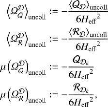 (50)
(50)
where  is the kth domain among the sorted ith scale factorsof uncollapsed domains satisfying
 (51)
(51)
and Eqs. (30)–(33) are used to evaluate  and
and  (ties in the median, if they occur, are upper weighted). The
  volume-weighted mean and median values for uncollapsed domains are positive, corresponding to negative
  , which tends to cause earlier collapse of overdensities and slower expansion of voids. Thus, if kinematical backreaction were artificially set to zero in all domains, as appears to be the case in Rácz et al. (2017) and is shown here in Fig. 9, then it would be reasonable for the faster expansion of voids to contribute to much stronger scale factor growth. In that case, larger scale (lower amplitude) initial overdensities would be sufficient to obtain aeff (13.8 Gyr) = 1, as can be seen in Fig. 9.
The values of the mean and median  values shown in Fig. 10 only sample uncollapsed domains, and are normalised globally (Wiegand & Buchert 2010, Eq. (10)), rather than per-domain (Eq. (42)). This implies that prior to virialisation, the mean should be constrained to be close to zero by the Stokes’ theorem T3 constraint on the global kinematical backreaction
  . This does appear to be the case in the upper panel of Fig. 10 at very early times, but the first virialisation events happen quickly, so
  quickly grows away from zero.
The spikiness of Fig. 10 (the vertical axis is logarithmic) is physically realistic: it emphasises the discontinuous nature of virialisation. Each time a domain collapses, it no longer contributes to  as defined for this figure. Forcing a smooth aEdS(t) (or aΛCDM(t)) global volume evolution artificially hides this spikiness. Unsurprisingly, the volume-weighted medians
  evolve muchmore smoothly, since the collapse of a domain shifts the median within the central part of the
  distribution, which is denser than the tails. For
  , these medians peak rapidly at about 0.03 and then gradually decay to the present.
As expected by Buchert (2005; see Sect. 1 above for more literature), the super-EdS aeff (t) is accompanied by emerging negative average curvature, as shown in Fig. 11. At the  scale (middle curve at early times), the volume-weighted mean
  for uncollapsed domains grows from zero to about 1 by about half the age of the Universe and then grows more slowly to about 1.5 by the present. The volume-weighted median
  also grows quickly to about 1.5 by t~ 4 Gyr, the same epoch, and then grows slowly to about 2 by the present. New observational tests will be needed to constrain recent emerging curvature such as that modelled here, since constraints that assume comoving non-evolving uniform curvature do not constrain evolving non-uniform mean curvature. Moreover, in this work, no distinction is made between volume-average (“bare”) Ω parameters and those likely to be observed from our Galaxy (“dressed”; Buchert & Carfora 2002, 2003), so more work will be needed to calculate parameters such as the detailed estimations for the Timescape model given in Nazer & Wiltshire (2015, Table II).
5.3 Dependence of super-EdS expansion on virialisation fraction fvir
Roukema et al. (2013) argued that virialisation and non-rigidity of voids constitute a key element to an emerging negative average curvature alternative to dark energy. The VQZA provides an ab initio model of this argument, so it should be possible to verify the relationship between super-EdS expansion and virialisation. The virialisation fraction (fraction of mass in virialised objects) can be estimated by counting the number Ncoll of domains  that have gravitationally collapsed at any given time and normalising:
 (52)
(52)
Figure 12 shows that at any fixed time, VQZA simulations run from independent realisations of initial conditions yield super-EdS expansion aeff ∕aEdS that correlate strongly with fvir. Spearman’s rank correlation ρ tests overwhelmingly confirm this, giving a probability p = 3 × 10⁻⁹, 10−9, and 10−6, of no correlation between fvir and aeff∕aEdS at the early,middle, and late times (as listed in Fig. 12), respectively.
Thus, unsurprisingly, silent virialisation leads to a strong correlation between the degree of virialisation fvir (t) that resultsfrom a given realisation of initial conditions at a given time t and the amount of super-EdS expansion aeff(t)∕aEdS(t) at that same epoch. Enforcement of Newtonian global expansion, as in standard cosmological N-body simulations, would destroy this correlation, since in that case aeff(t)∕aEdS(t) := 1 by definition.
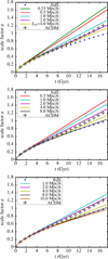 |
Fig. 7 Full box cube-root-of-total-volume scale factor aeff(t) evolution fortop: |


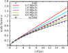 |
Fig. 8 As in Fig. 7, full box cube-root-of-total-volume scale factor aeff (t), for |


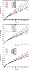 |
Fig. 9 As in Fig. 7, full box cube-root-of-total-volume scale factoraeff (t), but ignoring kinematical backreaction (setting |


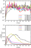 |
Fig. 10 Evolution of the volume-weighted mean (above) and median (below) globally normalised kinematical backreaction functional |

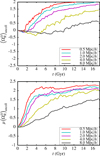 |
Fig. 11 Evolution of the volume-weighted mean (above) and median (below) globally normalised curvature functional |

 |
Fig. 12 Super-EdS ratio aeff∕aEdS versus virialisation fraction fvir for 100 VQZA simulations with |


5.4 N-body measurement of 
What happens when  is calculated from the Lagrangian domains in the evolving N-body simulation, as detailed in Sect. 3.7 above, where numerical noise plays a stronger role? Figs. 13 and 14 show the equivalent of Figs. 7 (middle) and 9 (top), respectively. (See Table 1 for software versions.)
Figures 9 (top) and 14, in which  is artificially set to zero, appear, by inspection, to be almost identical. This close correspondence provides a check on the numerical integration and coordination between software modules, since the former integration is carried out by calls from the INHOMOG library to the GSL routine GSL_ODEIV_STEP_RKF45, while the latter is carried out by the RAMSES-SCALAV routine UPDATE_AV_SCALARS_GLOBAL_MODULE with a hardwired version of the classical (non-adaptive) Runge–Kutta algorithm. The initial conditions were not set to be identical between these two panels, so the small differences indicate both cosmic variance and numerical error.
For more realistic calculations, when kinematical backreaction is not set to zero, Fig. 13 shows more complex behaviour than that in Fig. 7 (middle). The sequence of bigger scales  Mpc∕heff has slightly stronger aeff(t) than for the VQZA case. In contrast, for the sequence of smaller scales (
 Mpc∕heff) the aeff(t) growth is successively weaker. Cosmic variance is strong on these scales, so seeking an explanation from a small number of small simulations is not strongly justified: many competing numerical effects such as close-encounter scattering and softening may be involved. More importantly for the present work, a value of 1 ≲ L13.8∕Mpc∕heff ≲ 4 indicates consistency with the VQZA calculations. Future work on higher numbers of higher N simulations will enable a statistically more significant comparison between the analytical and numerical models of
  and their effects on aeff(t).
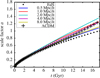 |
Fig. 13 As in Fig. 7 (middle), for N-body evolution and Lagrangian tracing of initial domains, for |


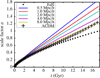 |
Fig. 14 As inFig. 9 (top), for N-body evolution and Lagrangian tracing of initial domains, for |


6 Discussion
6.1 Should global backreaction from T3 initial conditions be zero?
The scalar averaging equations, given in Sect. 3.5.1 together with Eq. (44), can be applied on any domain size, including the global volume, which in this work is T3, provided that the assumptions underlying the equations are satisfied. For flat space, given the definition of  in Eq. (16) and the flat space expression of the peculiar velocity gradient invariants as exact divergences in Eq. (11), it would appear that
  must be zero. Thus, Eq. (14) should yield aeff(t) ≡ aEdS(t), no matter what scale of
  is chosen, provided that the evolution of
  is calculated exactly. More realistically, in the present case
  is calculated using the QZA (Eqs. (30), (31)), so aeff (t) ≈ aEdS(t) should still be a good approximation, to the degree that Eqs. (30), (31) remain accurate at t, modulo Poisson noise contributed by combining many domains. Indeed, Fig. 1 shows that prior to virialisation, this approximation holds reasonably well in illustrative cases.
However, Eq. (14) and the definition of  normally used in the literature are derived for a pressureless perfect fluid, that is, “dust”, with no allowance for shell crossings or avoidance ofcollapse to a singularity. This is not a problem for studying non-linear gravitational collapse times of overdense objects, in which case these equations yield realistic estimates in a more elegant way than the usual alternatives (Ostrowski et al. 2017a,b; Ostrowski 2016; Ostrowski et al., in prep.). On the other hand, Eq. (14) (in its form stated above) is no longer valid once the final stages of gravitational collapse and virialisation have taken place. As
  in Eq. (14),
  via Eqs. (30) and (31) is not able to cancel self-gravity, so a literal interpretation of Eq. (14) would imply that
  .
.
In this sense, the global volume-averaging expressed in Eq. (44) is used in this work as an extension beyond the usual set of scalar averaging equations; the metric volumes are summed, but the choice of the  scale affects the result via virialisation.
Obviously, if the aim of calculations of this sort were to study EdS cosmology and to substitute a perfect fluid by a set of collisionless particles in which shell-crossings were allowed, then it would have to be possible to modify Eq. (14) by adding a virialisation term to the kinematical backreaction in order to prevent collapse to a singularity. For example, this could take the form of the dynamical backreaction proposed in Eqs. (13a), (13d) of Buchert (2001) (see also Yodzis 1974; Buchert 2018, footnote 7). To retain a global EdS expansion history, the new term would not only have to prevent collapsing domains from forming singularities, but would also have to correspondingly slow down the expansion rate of expanding domains, in order to retain a net EdS expansion rate during the post-virialisation phase.
The main aim of this work is a step towards relativistic cosmology rather than testing the consistency of Newtonian cosmology. The latter requires instant reaction at a distance, but the former is constrained by causality, making instantaneous reaction to virialisation unphysical. Thus, the approach defined in Definition 1 (Sect. 1) is retained for the present work. In other words, here, the QZA formulae for expanding regions are not modified nor supplemented in reaction to virialisation, and the resulting global volume evolution is not constrained to be Newtonian.
Moreover, since stable clustering is adopted for virialised domains, if we consider their volume-weighted curvature contributions to be negligible (either because the volumes are tiny, the curvature is weak, or both), then the negative curvature of the expanding domains will tend to yield an overall negative mean curvature, invalidating the derivation of the divergence expressions in Eq. (11) at late times, since a flat manifold is no longer a good approximation.
6.2 How can virialisation provide an order-unity dark-energy expansion?
How is it possible that stable clustering, which is typically thought of as a Newtonian statistical gravitational effect, can provide a reasonable relativistic approximation in this context? The reasoning above can be reworded as follows. Prior to virialisation, the QZA formulae provide a good cancellation between expansion and collapse compared to EdS evolution of the scale factor. At a virialisation event, the spatially contracting contribution of a virialised domain to the general cosmological volume evolution is cancelled, either by the stable clustering assumption or (in future work) using more detailed analytical models (Buchert 2001, 2018; Bolejko & Lasky 2008; Bolejko & Ferreira 2012). To better than an order of magnitude, about half the mass of any large volume today is located in virialised dark matter haloes. Thus, among the ensemble of domains on the non-linear, few-megaparsec scale, the domains that contribute about half the total mass have their gravitational roles cancelled, in the sense that the averaged Raychaudhuri equation, Eq. (14), is replaced by
 (53)
(53)
for those domains. Under an EdS constraint, expanding regions are forced to slow their expansion down in response to this virialisation.Relativistically interpreted, this would mean that the expanding, negatively curved regions are forced to slow down and flatten. Without the EdS constraint, that is, without modifying the QZA formula for expanding domains (or in other words, with the hypothesis that silent virialisation is a fair approximation), about half the mass that contributes to deceleration of the global, effective scale factor is effectively cancelled, in terms of its contribution to average deceleration. Thus, the cancelling of about half the deceleration results in volume acceleration. This effect (related to that of “finite infinity” regions: Ellis 1984; Wiltshire 2007a; Cox 2007) is overlooked in the standard approach because Eq. (44) (cubical averaging of domain-wise scale factors) is not normally used.
In this sense, the “new physics” that contributes significantly to dark energy is old physics – Newtonian virialisation – that is assumed to not have instantaneous effects at a distance. This could be described as non-compensation for virialisation. The global acceleration effect emerges indirectly from a statistical Newtonian particle effect via the combination of Eq. (14) for pre-virialisation average volume evolution (with Λ ≡ 0), Eq. (53) for virialised domains, and Eq. (44) to silently prevent the latter from affecting the former.
6.3 Caveats of the VQZA, the fluid model and vorticity
The accuracy of the VQZA depends on the accuracy of the assumptions stated in Definition 1, Sect. 1. For example, if propagation of relativistic constraints across domain boundaries implied that virialisation in one domain induced inaccuracy in the QZA formulae (Eqs. (11), (30), (31)) in one or more neighbouring domains, then this would lead to systematic error due to violation of the silent virialisation assumption of (ii) and (iv) of Definition 1. Other simplifying assumptions either stated above or implicit to the VQZA approach presented here include:
- (i)
a spacetime foliation that matches the EdS foliation at early times is assumed (proper time and coordinate time are not distinguished);
- (ii)
the difference between the sum of rest masses and the system mass is assumed to be negligible (see Adamek et al. 2016a,b, for an example of modelling Lorentzian effects);
- (iii)
Eqs. (14)–(16) are justified in the relativistic case under the assumption of zero vorticity;
- (iv)
there is assumed to be no shell-crossing prior to virialisation;
- (v)
althoughthe scale found to be of most interest is found to be
 , the calculations were performed (in particular see Fig. 7) down to
  , where it is clear that the zero vorticity and lack of shell-crossing assumptions could potentially lead to non-negligible correction terms.
Thus, as with each of the other approaches towards general-relativistic cosmological simulations published so far (see Sect. 1), the approximations and simplifying assumptions of this approach have to be studied further in order to judge how much they affect the results.
7 Conclusion
This work presents the first in a series of cosmological expansion modelling improvements. These aim to incorporate successively more elements towards obtaining general-relativistically valid N-body simulations in which the effective expansion rate is calculated from local structure formation rather than inserted arbitrarily. A key element of the present work in obtaining super-EdS expansion is described inSect. 2 and illustrated quantitatively in Sect. 4. This is the virialisation– Zel’dovich approximation (Definition 1, Sect. 1), in which locally Newtonian expansion modelled by the QZA in combinationwith virialisation modelled under the stable clustering hypothesis together imply super-EdS evolution of the effective expansion rate.
The standard FLRW structure formation alternative to the VQZA can be summarised as follows:
- (i)
prior to a collapse/virialisation event, the Lagrangian per-domain average scale factor evolution is implicitly modelled to be smooth for both the collapsing domain and the expanding domain;
- (ii)
the final stages of a gravitational collapse and virialisation event are very sudden in comparison with cosmological time scales;
- (iii)
the global scale factor evolution is assumed to be smooth (FLRW) passing from times prior to the collapse/virialisation event through to times following the event;
- (iv)
assumptions (i) + (ii) + (iii) together imply that at least one expanding domain
 must undergo a sudden drop in acceleration
  when the collapse/virialisation event occurs, in order to compensate for the latter; smooth expansion would violate either (ii) or (iii); in the case of a biscale model, the mean spatial 3-Ricci curvature (in a relativistic interpretation) of the expanding domain must suddenly switch from negative curvature to zero curvature.
The hypothesis adopted here is that (iv) is relativistically unrealistic (as shown by the solid curves in Fig. 2 for biscale examples). This motivates the VQZA, in which (i) and (ii) hold, but (iii) is violated to the degree that any collapse/virialisation process is accepted to be a sudden event, and to be silent – without a significant sudden effect on expanding domains. Thus, the VQZA avoids (iv) the non-differentiability of  for expanding domains
  . In other words, we postulate that smoothness in volume growth of the expanding domain, as approximated in the QZA, is relativistically more accurate than smoothness in global mean volume growth in situations in which collapse terminates suddenly in a small, already greatly contracted domain. In Sect. 4, this argument is illustrated analytically and numerically with a biscale model that shows the sudden change required to happen in the expanding domain in the standard model.
The consequences of the VQZA were examined here for a more generic case, by partitioning general N-body simulation initial conditions into initially cubical domains.
- (i)
We introduced (Sects. 3.4.1, 3.4.2) a method of estimating numerical error in velocity gradient numerical estimates by applying Stokes’ theorem over S1. We found (Sect. 5.1) that for a simulation with Lbox∕LN = 128, structure scales of Lbox∕64 or greater had S∕N ratios in the accuracy of DTFE determination of the velocity gradient invariants I and II of about ten or higher, except when attempting sub–mean-interparticle-separation sampling at LDTFE = LN∕2.
- (ii)
Based onour VQZA simulations (Figs. 7, 8), we consider
 to be a reasonable representation of the averaging scale
  which provides the optimal amount of super-EdS scale factor evolution to match observations as represented by an
ΛCDM proxy. The error represents our estimate of systematic error associated with changing the box (T3
fundamental domain), DTFE and particle resolution scales, and running 100 VQZA simulations of size
N = 2563
at each relevant set of scales. Our largest box size simulations yield L13.8 = 2.56 ± 0.01 Mpc∕heff, where the error is one standard deviation (not the standard error in the mean), but since these have low ratios
which provides the optimal amount of super-EdS scale factor evolution to match observations as represented by an
ΛCDM proxy. The error represents our estimate of systematic error associated with changing the box (T3
fundamental domain), DTFE and particle resolution scales, and running 100 VQZA simulations of size
N = 2563
at each relevant set of scales. Our largest box size simulations yield L13.8 = 2.56 ± 0.01 Mpc∕heff, where the error is one standard deviation (not the standard error in the mean), but since these have low ratios
 , it is likely that systematic, resolution-related error is greater than this random error.
 - (iii)
This super-EdS scale factor evolution is associated with kinematical backreaction and curvature normalised functionals
 and
and  , respectively, whose volume-weighted means and medians for uncollapsed domains are mostly positive throughout cosmic history (Figs. 10, 11). Kinematical backreaction is strongest at early times, with
 reaching a median value of about 0.03 at t ≈ 2 Gyr and then dropping gradually towards zero. The recent emergence of average negative curvature is confirmed in these calculations, with the
  mean and median values for uncollapsed domains growing to about 1.5 to 2, respectively, by the present.
 - (iv)
Cosmic variance, as represented by independent realisations of initial conditions, gives different numbers of collapsed objects at a given cosmological time, and thus virialisation fractions fvir, for a given choice of
 . The super-EdS scale factor ratio aeff∕aEdS
is very strongly correlated with fvir
(Sect. 5.3, Fig. 12).
. The super-EdS scale factor ratio aeff∕aEdS
is very strongly correlated with fvir
(Sect. 5.3, Fig. 12). - (v)
Artificially setting
 gives
gives  (Figs. 9, 14). This is the result that we would expect from Rácz et al. (2017)’s approach.
 - (vi)
Small numbers of small exploratory simulations with numerical estimation of
 at every major time step give rough agreement with the VQZA L13.8
scale (Fig. 13).
at every major time step give rough agreement with the VQZA L13.8
scale (Fig. 13).
Thus, from EdS initial conditions, dropping the decoupling hypothesis and estimating spatial expansion using the VQZA provides sufficient dark-energy–free average expansion by the standard age of the Universe estimate, for an averaging  scale of
  . This estimate is just a factor of about three lower than (more non-linear than) the 8 Mpc∕heff scale at which the σ8 normalisation of the initial power spectrum of density perturbations in flat space Pk is normally defined. The historically important non-linearity scale, the r0 scale in the two-point spatial auto-correlation function of galaxies, at which the excess probability of finding a pair of galaxies is unity, is close in value. This was estimated over four decades ago (Peebles 1974) as 5 Mpc∕heff ≲ r0 ≲ 10 Mpc∕heff (Peebles & Hauser 1974, Eq. (48)). In this presentation of the VQZA, we set σ8 appropriate for an early-epoch Planck-parametrised ΛCDM model (Sect. 3.3). Since silent virialisation is the key driver of the super-EdS expansion that we find here, it is unsurprising that (i) L13.8, (ii) the 8 Mpc∕heff scale at which σ8 is not far from unity, and (iii) the galaxy two-point auto-correlation function zero point r0 are close in value to one another.
This work provides a step towards correcting standard N-body simulations for the general-relativistic constraints imposed by scalar averaging. This work is too preliminary to provide observational predictions at comparable precision to that of the ΛCDM model. Future work will need to include: inhomogeneous spatial curvature for calculating averages; curvature effects of particle movement; feedback of the global expansion rate on the effective background model growth rate ξ(t); improvement beyond the QZA, since the QZA is only a first-order approximation (Buchert et al. 2013, Sects. IV, V; see Alles et al. 2015), in particular by taking into account an effective background with evolving average curvature; and ray-tracing for calculating luminosity distances and angular diameter distances through inhomogeneously curved spatial sections (see, for example, Sikora & Głód 2017, in which the effective scale factor of the scalar-averaging averaging approach is found to be a good match to detailed ray-tracing calculations in a specific cosmological inhomogeneous metric).
Nevertheless, it seems reasonable to consider this work to be more accurate than the standard model: sudden, acausal switches in curvature and expansion rates in expanding regions that contain no singular spacetime events would be relativistically surprising.
Acknowledgements
Thank you to Jérémy Blaizot, Krzysztof Bolejko, Justyna Borkowska, Thomas Buchert, Mikołaj Korzyński, Bartosz Lew, Jan Ostrowski, Pierre Mourier, Yann Rasera, Joakim Rosdahl, Quentin Vigneron, David Wiltshire, and an anonymous referee for useful comments. A part of this project was funded by the National Science Centre, Poland, under grant 2014/13/B/ST9/00845. Part of this work consists of research conducted within the scope of the HECOLS International Associated Laboratory, supported in part by the Polish NCN grant Dec-2013/08/M/ST9/00664. A part of this project has made use of computations made under grant 314 of the Poznań Supercomputing and Networking Center (PSNC). This work has used the free-licensed GNU OCTAVE package (Eaton et al. 2014).
Appendix A Newtonian velocity gradient invariants
Here we provide a script (Appendix A Ostrowski 2016) that can be run using the free-licensed computer algebra system MAXIMA, version v.5.32.18, in order to confirm the equivalence of the expressions in Eq. (11). The three PRINTF statements at the end should yield “0” to show algebraic equivalences.
Appendix B Variance of the third invariant ![Mathematical equation: $\mathbb{E}[\left<\mathsf{III}_{{\vec i}}\right>^2_{{\cal B}_R} ]$](/articles/aa/full_html/2018/02/aa31400-17/aa31400-17-eq290.png)
As in Appendix B of BKS, for a Gaussian density field of power spectrum Pi (k) for a Fourier mode k of amplitude k := |k|, we label independentmodes ki, for 1 ≤ i ≤ 6, and estimate the ensemble mean ![Mathematical equation: $\mathbb{E}[.]$](/articles/aa/full_html/2018/02/aa31400-17/aa31400-17-eq291.png) by using thespatial mean. The six-point correlation function can be factorised by finding all distinct triples of pairs, similarly to (C17) of BKS00,
by using thespatial mean. The six-point correlation function can be factorised by finding all distinct triples of pairs, similarly to (C17) of BKS00,
![Mathematical equation: \begin{align*} \mathbb{E}&[ \tilde{\delta}_{{\vec i}}({\vec k}_1) \tilde{\delta}_{{\vec i}}({\vec k}_2) \tilde{\delta}_{{\vec i}}({\vec k}_3) \tilde{\delta}_{{\vec i}}({\vec k}_4) \tilde{\delta}_{{\vec i}}({\vec k}_5) \tilde{\delta}_{{\vec i}}({\vec k}_6) ]= \nonumber \\ & \;\; P_{{\vec i}}(k_1) P_{{\vec i}}(k_3) P_{{\vec i}}(k_5) \,\delta^D({\vec k}_1 + {\vec k}_2) \, \delta^D({\vec k}_3 + {\vec k}_4) \, \delta^D({\vec k}_5 + {\vec k}_6) \, \nonumber \\ &\;+ P_{{\vec i}}(k_1) P_{{\vec i}}(k_3) P_{{\vec i}}(k_4) \,\delta^D({\vec k}_1 + {\vec k}_2) \, \delta^D({\vec k}_3 + {\vec k}_5) \, \delta^D({\vec k}_4 + {\vec k}_6) \, \nonumber \\ &\;+ P_{{\vec i}}(k_1) P_{{\vec i}}(k_3) P_{{\vec i}}(k_4) \,\delta^D({\vec k}_1 + {\vec k}_2) \, \delta^D({\vec k}_3 + {\vec k}_6) \, \delta^D({\vec k}_4 + {\vec k}_5) \, \nonumber \\ &\;+ P_{{\vec i}}(k_1) P_{{\vec i}}(k_2) P_{{\vec i}}(k_5) \,\delta^D({\vec k}_1 + {\vec k}_3) \, \delta^D({\vec k}_2 + {\vec k}_4) \, \delta^D({\vec k}_5 + {\vec k}_6) \, \nonumber \\ &\;+ P_{{\vec i}}(k_1) P_{{\vec i}}(k_2) P_{{\vec i}}(k_4) \,\delta^D({\vec k}_1 + {\vec k}_3) \, \delta^D({\vec k}_2 + {\vec k}_5) \, \delta^D({\vec k}_4 + {\vec k}_6) \, \nonumber \\ &\;+ P_{{\vec i}}(k_1) P_{{\vec i}}(k_2) P_{{\vec i}}(k_4) \,\delta^D({\vec k}_1 + {\vec k}_3) \, \delta^D({\vec k}_2 + {\vec k}_6) \, \delta^D({\vec k}_4 + {\vec k}_5) \, \nonumber \\ &\;+ P_{{\vec i}}(k_1) P_{{\vec i}}(k_2) P_{{\vec i}}(k_5) \,\delta^D({\vec k}_1 + {\vec k}_4) \, \delta^D({\vec k}_2 + {\vec k}_3) \, \delta^D({\vec k}_5 + {\vec k}_6) \, \nonumber \\ &\;+ P_{{\vec i}}(k_1) P_{{\vec i}}(k_2) P_{{\vec i}}(k_3) \,\delta^D({\vec k}_1 + {\vec k}_4) \, \delta^D({\vec k}_2 + {\vec k}_5) \, \delta^D({\vec k}_3 + {\vec k}_6) \, \nonumber \\ &\;+ P_{{\vec i}}(k_1) P_{{\vec i}}(k_2) P_{{\vec i}}(k_3) \,\delta^D({\vec k}_1 + {\vec k}_4) \, \delta^D({\vec k}_2 + {\vec k}_6) \, \delta^D({\vec k}_3 + {\vec k}_5) \, \nonumber \\ &\;+ P_{{\vec i}}(k_1) P_{{\vec i}}(k_2) P_{{\vec i}}(k_4) \,\delta^D({\vec k}_1 + {\vec k}_5) \, \delta^D({\vec k}_2 + {\vec k}_3) \, \delta^D({\vec k}_4 + {\vec k}_6) \, \nonumber \\ &\;+ P_{{\vec i}}(k_1) P_{{\vec i}}(k_2) P_{{\vec i}}(k_3) \,\delta^D({\vec k}_1 + {\vec k}_5) \, \delta^D({\vec k}_2 + {\vec k}_4) \, \delta^D({\vec k}_3 + {\vec k}_6) \, \nonumber \\ &\;+ P_{{\vec i}}(k_1) P_{{\vec i}}(k_2) P_{{\vec i}}(k_3) \,\delta^D({\vec k}_1 + {\vec k}_5) \, \delta^D({\vec k}_2 + {\vec k}_6) \, \delta^D({\vec k}_3 + {\vec k}_4) \, \nonumber \\ &\;+ P_{{\vec i}}(k_1) P_{{\vec i}}(k_2) P_{{\vec i}}(k_4) \,\delta^D({\vec k}_1 + {\vec k}_6) \, \delta^D({\vec k}_2 + {\vec k}_3) \, \delta^D({\vec k}_4 + {\vec k}_5) \, \nonumber \\ &\;+ P_{{\vec i}}(k_1) P_{{\vec i}}(k_2) P_{{\vec i}}(k_3) \,\delta^D({\vec k}_1 + {\vec k}_6) \, \delta^D({\vec k}_2 + {\vec k}_4) \, \delta^D({\vec k}_3 + {\vec k}_5) \, \nonumber \\ &\;+ P_{{\vec i}}(k_1) P_{{\vec i}}(k_2) P_{{\vec i}}(k_3) \,\delta^D({\vec k}_1 + {\vec k}_6) \, \delta^D({\vec k}_2 + {\vec k}_5) \, \delta^D({\vec k}_3 + {\vec k}_4) \, ,\end{align*}](/articles/aa/full_html/2018/02/aa31400-17/aa31400-17-eq292.png) (B.1)
(B.1)
where δD is the Dirac delta function. Use of (B.1) together with (C9) and (C10) of BKS, where  is a ball of radius R and
  is the Fourier transform of the normalised top-hat window function WR, leads to
![Mathematical equation: \begin{align*} \mathbb{E}&[\left<{\vec III}_{{\vec i}}\right>^2_{{\cal B}_R} ]= \nonumber \\ & {32\, \pi^6} \int_{\mathbb{R}^3} \mathrm{d}^3 k_1 \int_{\mathbb{R}^3} \mathrm{d}^3 k_2 \int_{\mathbb{R}^3} \mathrm{d}^3 k_3 \nonumber \\ &\; { \frac{{ \widetilde{W}_R\left(| {{\vec k}}_1 + {{\vec k}}_ 2 + {{\vec k}}_3 |\right)}^2\, P_{{\vec i}}(k_1) P_{{\vec i}}(k_2) P_{{\vec i}}(k_3)} { 3\, { {k}_1}^4\, { {k}_2}^4\, { {k}_3}^4} } \; \nonumber \\ &\;\times \left[{ {k}_1}^2\, { {k}_2}^2\, { {k}_3}^2-3\, { ({\vec k}_2 \cdot {\vec k}_3)}^2\, { {k}_1}^2+2\, { ({\vec k}_1 \cdot {\vec k}_2)}\, { ({\vec k}_1 \cdot {\vec k}_3)}\, { ({\vec k}_2 \cdot {\vec k}_3)}\right] \; \nonumber \\ &\; \times\left[{ {k}_1}^2\, { {k}_2}^2\, { {k}_3}^2-{ ({\vec k}_1 \cdot {\vec k}_2)}^2\, { {k}_3}^2- { ({\vec k}_1 \cdot {\vec k}_3)}^2\, { {k}_2}^2-{ ({\vec k}_2 \cdot {\vec k}_3)}^2\, { {k}_1}^2 \right. \nonumber \\ &\; +\left. 2 \vphantom{{{\vec k}_9}^9} \, { ({\vec k}_1 \cdot {\vec k}_2)}\, { ({\vec k}_1 \cdot {\vec k}_3)}\, { ({\vec k}_2 \cdot {\vec k}_3)}\right]\end{align*}](/articles/aa/full_html/2018/02/aa31400-17/aa31400-17-eq295.png) (B.2)
(B.2)
rather than the original (C20)–(C22). Terms induced by (B.1) that involve  cancel exactly.
These expressions have been derived with the help of GNU OCTAVE and the free-licensed computer algebra system MAXIMA and tested numerically using numerical 18-dimensional integration with two sample points per dimension, performed with the GNU Scientific Library.
References
- Adamek, J., Clarkson, C., Durrer, R., & Kunz, M. 2015, Phys. Rev. Lett., 114, 051302 [NASA ADS] [CrossRef] [Google Scholar]
- Adamek, J., Daverio, D., Durrer, R., & Kunz, M. 2016a, Nat. Phys., 12, 346 [CrossRef] [Google Scholar]
- Adamek, J., Daverio, D., Durrer, R., & Kunz, M. 2016b, J. Cosmol. Astropart. Phys., 7, 053 [NASA ADS] [CrossRef] [Google Scholar]
- Ade, P. A. R., Aghanim, N., Armitage-Caplan, C., et al. 2014, A&A, 571, A26 [NASA ADS] [CrossRef] [EDP Sciences] [Google Scholar]
- Ade, P. A. R., Aghanim, N., Arnaud, M., et al. 2016, A&A, 594, A13 [NASA ADS] [CrossRef] [EDP Sciences] [Google Scholar]
- Alles, A., Buchert, T., Al Roumi, F., & Wiegand, A. 2015, Phys. Rev. D, 92, 023512 [NASA ADS] [CrossRef] [Google Scholar]
- Aragón-Calvo, M. A., Platen, E., van de Weygaert, R., & Szalay, A. S. 2010a, ApJ, 723, 364 [NASA ADS] [CrossRef] [Google Scholar]
- Aragon-Calvo, M. A., Shandarin, S. F., &Szalay, A. 2010b, ArXiv e-prints [arxiv:1006.4178] [Google Scholar]
- Aslanyan, G., & Manohar, A. V. 2012, J. Cosmol. Astropart. Phys., 6, 3 [NASA ADS] [CrossRef] [Google Scholar]
- Aurich, R. 2015, MNRAS, 452, 1493 [NASA ADS] [CrossRef] [Google Scholar]
- Bagla, J. S. 2005, Current Science, 88, 1088 [Google Scholar]
- Barbosa, R. M., Chirinos Isidro, E. G., Zimdahl, W., & Piattella, O. F. 2016, Gen. Relativity Gravitation, 48, 51 [Google Scholar]
- Bensby, T., Yee, J. C., Feltzing, S., et al. 2013, A&A, 549, A147 [NASA ADS] [CrossRef] [EDP Sciences] [Google Scholar]
- Bentivegna, E., & Bruni, M. 2016, Phys. Rev. Lett., 116, 251302 [NASA ADS] [CrossRef] [Google Scholar]
- Bernardeau, F., & van de Weygaert, R. 1996, MNRAS, 279, 693 [NASA ADS] [CrossRef] [Google Scholar]
- Bertschinger, E. 2001, ApJS, 137, 1 [NASA ADS] [CrossRef] [Google Scholar]
- Bildhauer, S., Buchert, T., & Kasai, M. 1992, A&A, 263, 23 [NASA ADS] [Google Scholar]
- Blanchard, A., Douspis, M., Rowan-Robinson, M., & Sarkar, S. 2003, A&A, 412, 35 [NASA ADS] [CrossRef] [EDP Sciences] [Google Scholar]
- Bolejko, K. 2009, Gen. Relativity Gravitation, 41, 1585 [NASA ADS] [CrossRef] [Google Scholar]
- Bolejko, K. 2017a, J. Cosmol. Astropart. Phys., 06, 025 [NASA ADS] [CrossRef] [Google Scholar]
- Bolejko, K. 2017b, ArXiv e-prints [arxiv:1707.01800] [Google Scholar]
- Bolejko, K. 2017c, Class. Quant. Grav., 35, 024003 [NASA ADS] [CrossRef] [Google Scholar]
- Bolejko, K., & Célérier, M.-N. 2010, Phys. Rev. D, 82, 103510 [NASA ADS] [CrossRef] [Google Scholar]
- Bolejko, K., & Ferreira, P. G. 2012, J. Cosmol. Astropart. Phys., 5, 003 [NASA ADS] [CrossRef] [Google Scholar]
- Bolejko, K., & Lasky, P. D. 2008, MNRAS, 391, L59 [NASA ADS] [Google Scholar]
- Bondi, H. 1947, MNRAS, 107, 410 [NASA ADS] [CrossRef] [Google Scholar]
- Bryan, G. L., & Norman, M. L. 1998, ApJ, 495, 80 [NASA ADS] [CrossRef] [Google Scholar]
- Buchert, T. 1994, MNRAS, 267, 811 [NASA ADS] [Google Scholar]
- Buchert, T. 2000a, in Proceedings of the ninth workshop on general relativity and gravitation, Hiroshima November 3–6, 1999, eds. Y. Eriguchi, T. Futamase, A. Hosoya, et al. (Hiroshima: Physics Department, Hiroshima University), 306 [Google Scholar]
- Buchert, T. 2000b, Gen. Rel. Grav., 32, 105 [NASA ADS] [CrossRef] [MathSciNet] [Google Scholar]
- Buchert, T. 2001, Gen. Rel. Grav., 33, 1381 [NASA ADS] [CrossRef] [Google Scholar]
- Buchert, T. 2005, Class. Quant. Grav., 22, L113 [NASA ADS] [CrossRef] [Google Scholar]
- Buchert, T. 2008, Gen. Rel. Grav., 40, 467 [NASA ADS] [CrossRef] [MathSciNet] [Google Scholar]
- Buchert, T. 2011, Class. Quant. Grav., 28, 164007 [NASA ADS] [CrossRef] [Google Scholar]
- Buchert, T. 2018, MNRAS, 473, L46 [NASA ADS] [CrossRef] [Google Scholar]
- Buchert, T., & Carfora, M. 2002, Class. Quant. Grav., 19, 6109 [NASA ADS] [CrossRef] [Google Scholar]
- Buchert, T., & Carfora, M. 2003, Phys. Rev. Lett., 90, 031101 [NASA ADS] [CrossRef] [Google Scholar]
- Buchert, T., & Carfora, M. 2008, Class. Quant. Grav., 25, 195001 [NASA ADS] [CrossRef] [MathSciNet] [Google Scholar]
- Buchert, T., & Ehlers, J. 1997, A&A, 320, 1 [NASA ADS] [Google Scholar]
- Buchert, T., Kerscher, M., & Sicka, C. 2000, Phys. Rev. D, 62, 043525 [NASA ADS] [CrossRef] [Google Scholar]
- Buchert, T., Nayet, C., & Wiegand, A. 2013, Phys. Rev. D, 87, 123503 [NASA ADS] [CrossRef] [Google Scholar]
- Buchert, T., & Ostermann, M. 2012, Phys. Rev. D, 86, 023520 [NASA ADS] [CrossRef] [Google Scholar]
- Buchert, T., & Räsänen, S. 2012, Ann. Rev. Nucl. Part. Sci., 62, 57 [NASA ADS] [CrossRef] [Google Scholar]
- Cautun, M. C., & van de Weygaert, R. 2011, ArXiv e-prints [arxiv:1105.0370] [Google Scholar]
- Chiesa, M., Maino, D., & Majerotto, E. 2014, J. Cosmol. Astropart. Phys., 12, 49 [NASA ADS] [CrossRef] [Google Scholar]
- Chirinos Isidro, E. G., Barbosa, R. M., Piattella, O. F., & Zimdahl, W. 2017, Class. Quant. Grav., 34, 035001 [NASA ADS] [CrossRef] [Google Scholar]
- Coley, A. A. 2010, Class. Quant. Grav., 27, 245017 [NASA ADS] [CrossRef] [Google Scholar]
- Cox, D. P. G. 2007, Gen. Rel. Grav., 39, 87 [NASA ADS] [CrossRef] [Google Scholar]
- Daverio, D., Dirian, Y., & Mitsou, E. 2017, Class. Quant. Grav., 34, 237001 [NASA ADS] [CrossRef] [Google Scholar]
- Dehnen, W., & Read, J. I. 2011, Eur. Phys. J. Plus, 126, 55 [CrossRef] [Google Scholar]
- Duley, J. A. G., Nazer, M. A., & Wiltshire, D. L. 2013, Class. Quant. Grav., 30, 175006 [NASA ADS] [CrossRef] [Google Scholar]
- Eaton, J. W., Bateman, D., Hauberg, S., & Wehbring, R. 2014, GNU Octave version 3.8.1 manual: a high-level interactive language for numerical computations (CreateSpace Independent Publishing Platform) [Google Scholar]
- Ehlers, J., & Buchert, T. 1997, Gen. Rel. Grav., 29, 733 [NASA ADS] [CrossRef] [Google Scholar]
- Eisenstein, D. J., & Hu, W. 1998, ApJ, 496, 605 [NASA ADS] [CrossRef] [Google Scholar]
- Eke, V. R., Cole, S., & Frenk, C. S. 1996, MNRAS, 282, 263 [NASA ADS] [CrossRef] [Google Scholar]
- Ellis, G. F. R. 1984, in General Relativity and Gravitation, eds. B. Bertotti, F. De Felice, & A. Pascolini, 215 [Google Scholar]
- Ellis, G. F. R., & Gibbons, G. W. 2014, Class. Quant. Grav., 31, 025003 [NASA ADS] [CrossRef] [Google Scholar]
- Ellis, G. F. R., & Stoeger, W. 1987, Class. Quant. Grav., 4, 1697 [NASA ADS] [CrossRef] [Google Scholar]
- Ellis, G. F., & Tsagas, C. G. 2002, Phys. Rev. D, 66, 124015 [NASA ADS] [CrossRef] [Google Scholar]
- Friedmann, A. 1923, Mir kak prostranstvo i vremya (The Universe as Space and Time) (Petrograd: Academia) [Google Scholar]
- Friedmann, A. 1924, Zeitschr. Phys., 21, 326 [Google Scholar]
- Giblin, Jr J. T., Mertens, J. B., & Starkman, G. D. 2016a, Phys. Rev. Lett., 116, 251301 [NASA ADS] [CrossRef] [Google Scholar]
- Giblin, Jr J. T., Mertens, J. B., & Starkman, G. D. 2016b, ApJ, 833, 247 [NASA ADS] [CrossRef] [Google Scholar]
- Guillet, T., & Teyssier, R. 2011, J. Comput. Phys., 230, 4756 [Google Scholar]
- Hunt, P., & Sarkar, S. 2007, Phys. Rev. D, 76, 123504 [NASA ADS] [CrossRef] [Google Scholar]
- Kai, T., Kozaki, H., Nakao, K., Nambu, Y., & Yoo, C. 2007, Prog. Theor. Phys., 117, 229 [NASA ADS] [CrossRef] [MathSciNet] [Google Scholar]
- Kaiser, N. 2017, MNRAS, 469, 744 [NASA ADS] [Google Scholar]
- Kasai, M. 1995, Phys. Rev. D, 52, 5605 [NASA ADS] [CrossRef] [Google Scholar]
- Kašpar, P., & Svítek, O. 2014, Class. Quant. Grav., 31, 095012 [NASA ADS] [CrossRef] [Google Scholar]
- Kennel, M. B. 2004, ArXiv e-prints [arxiv:physics/0408067] [Google Scholar]
- Krasinski, A. 1981, Gen. Rel. Grav., 13, 1021 [Google Scholar]
- Krasinski, A. 1982, in The Birth of the Universe, eds. J. Audouze, & J. Tran Thanh van, 15 [Google Scholar]
- Krasinski, A. 1983, Gen. Rel. Grav., 15, 673 [Google Scholar]
- Lacey, C., & Cole, S. 1993, MNRAS, 262, 627 [NASA ADS] [CrossRef] [Google Scholar]
- Larena, J., Alimi, J.-M., Buchert, T., Kunz, M., & Corasaniti, P.-S. 2009, Phys. Rev. D, 79, 083011 [NASA ADS] [CrossRef] [Google Scholar]
- Lavinto, M., Räsänen, S., & Szybka, S. J. 2013, J. Cosmol. Astropart. Phys., 12, 51 [NASA ADS] [CrossRef] [Google Scholar]
- Lemaître, G. 1927, Ann. de la Soc. Sc. de Brux., 47, 49 [Google Scholar]
- Lemaître, G. 1931, MNRAS, 91, 483 [NASA ADS] [Google Scholar]
- Lemaître, G. 1933, Ann. de la Soc. Sc. de Brux., 53, 51 [Google Scholar]
- Macpherson, H. J., Lasky, P. D., & Price, D. J. 2017, Phys. Rev. D, 95, 064028 [NASA ADS] [CrossRef] [Google Scholar]
- Matarrese, S., Pantano, O., & Saez, D. 1994a, MNRAS, 271, 513 [NASA ADS] [CrossRef] [Google Scholar]
- Matarrese, S., Pantano, O., & Saez, D. 1994b, Phys. Rev. Lett., 72, 320 [NASA ADS] [CrossRef] [MathSciNet] [PubMed] [Google Scholar]
- Matarrese, S., & Terranova, D. 1996, MNRAS, 283, 400 [NASA ADS] [CrossRef] [Google Scholar]
- Morita, M., Nakamura, K., & Kasai, M. 1998, Phys. Rev. D, 57, 6094 [NASA ADS] [CrossRef] [Google Scholar]
- Nadathur, S., & Sarkar, S. 2011, Phys. Rev. D, 83, 063506 [NASA ADS] [CrossRef] [Google Scholar]
- Nambu, Y., & Tanimoto, M. 2005, ArXiv e-prints, [arXiv:gr-qc/0507057] [Google Scholar]
- Nazer, M. A., & Wiltshire, D. L. 2015, Phys. Rev. D, 91, 063519 [NASA ADS] [CrossRef] [Google Scholar]
- Ostrowski, J. J. 2016, Ph.D. Thesis, Toruń Centre for Astronomy, Faculty of Physics, Astronomy and Informatics Nicolaus Copernicus University, Torun Poland [Google Scholar]
- Ostrowski, J. J., Buchert, T., & Roukema, B. F. 2017a, in Proceedings of the Fourteenth Marcel Grossmann Meeting on General Relativity, 12–18 July 2015, Rome, eds. M. Bianchi, R. T. Jantzen, & R. Ruffni (Singapore: World Scientific), [arXiv:1602.00302] [Google Scholar]
- Ostrowski, J. J., Buchert, T., & Roukema, B. F. 2017b, Acta Physica Polonica B Proceedings Supplement, 10, 407 [NASA ADS] [CrossRef] [Google Scholar]
- Park, C., Pranav, P., Chingangbam, P., et al. 2013, J. Korean Astron. Soc., 46, 125 [NASA ADS] [CrossRef] [Google Scholar]
- Peebles, P. J. E. 1974, ApJ, 189, L51 [NASA ADS] [CrossRef] [Google Scholar]
- Peebles, P. J. E. 1980, Large-Scale Structure of the Universe (Princeton University Press) [Google Scholar]
- Peebles, P. J. E., & Hauser, M. G. 1974, ApJS, 28, 19 [NASA ADS] [CrossRef] [Google Scholar]
- Pranav, P., Edelsbrunner, H., van de Weygaert, R., et al. 2017, MNRAS, 465, 4281 [NASA ADS] [CrossRef] [Google Scholar]
- Prunet, S., Pichon, C., Aubert, D., et al. 2008, ApJS, 178, 179 [NASA ADS] [CrossRef] [Google Scholar]
- Rácz, G., Dobos, L., Beck, R., Szapudi, I., & Csabai, I. 2017, MNRAS, 469, L1 [NASA ADS] [CrossRef] [Google Scholar]
- Räsänen, S. 2004, J. Cosmol. Astropart. Phys., 2, 003 [NASA ADS] [CrossRef] [Google Scholar]
- Räsänen, S. 2006, J. Cosmol. Astropart. Phys., 11, 003 [NASA ADS] [CrossRef] [Google Scholar]
- Räsänen, S. 2008, J. Cosmol. Astropart. Phys., 4, 026 [NASA ADS] [CrossRef] [Google Scholar]
- Robertson, H. P. 1935, ApJ, 82, 284 [NASA ADS] [CrossRef] [Google Scholar]
- Roukema, B. F., Ostrowski, J. J., & Buchert, T. 2013, J. Cosmol. Astropart. Phys., 10, 043 [NASA ADS] [CrossRef] [Google Scholar]
- Roukema, B. F., France, M. J., Kazimierczak, T. A., & Buchert, T. 2014, MNRAS, 437, 1096 [NASA ADS] [CrossRef] [Google Scholar]
- Roukema, B. F., Buchert, T., Ostrowski, J. J., & France, M. J. 2015, MNRAS, 448, 1660 [NASA ADS] [CrossRef] [Google Scholar]
- Roukema, B. F., Buchert, T., Fujii, H., & Ostrowski, J. J. 2016, MNRAS, 456, L45 [NASA ADS] [CrossRef] [Google Scholar]
- Roukema, B. F., Mourier, P., Buchert, T., & Ostrowski, J. J. 2017, A&A, 598, A111 [NASA ADS] [CrossRef] [EDP Sciences] [Google Scholar]
- Roy, X., Buchert, T., Carloni, S., & Obadia, N. 2011, Class. Quant. Grav., 28, 165004 [NASA ADS] [CrossRef] [Google Scholar]
- Schaap, W. E., & van de Weygaert, R. 2000, A&A, 363, L29 [NASA ADS] [Google Scholar]
- Sikora, S., & Głód, K. 2017, Phys. Rev. D, 95, 063517 [NASA ADS] [CrossRef] [Google Scholar]
- Sousbie, T. 2011, MNRAS, 414, 350 [NASA ADS] [CrossRef] [Google Scholar]
- Steiner, F. 2016, ArXiv e-prints [arxiv:1608.03133] [Google Scholar]
- Stichel, P. C. 2016, ArXiv e-prints [arxiv:1601.07030] [Google Scholar]
- Sussman, R. A., Hidalgo, J. C., Dunsby, P. K. S., & German, G. 2015, Phys. Rev. D, 91, 063512 [NASA ADS] [CrossRef] [Google Scholar]
- Szekeres, P. 1975, Communications in Mathematical Physics, 41, 55 [Google Scholar]
- Taylor, E. F., & Wheeler, J. A. 1992, Spacetime physics–Introduction to special relativity (2nd edn.) (W.H. Freeman and Co.) [Google Scholar]
- Teyssier, R. 2002, A&A, 385, 337 [NASA ADS] [CrossRef] [EDP Sciences] [Google Scholar]
- Tolman, R. C. 1934, Proc. Nat. Acad. Sci., 20, 169 [NASA ADS] [CrossRef] [Google Scholar]
- van de Weygaert, R., & Schaap, W. 2009, in Data Analysis in Cosmology, eds. V. J. Martínez, E. Saar, E. Martínez-González, & M.-J. Pons-Bordería (Berlin: Springer Verlag), Lect. Not. Phys., 665, 291 [NASA ADS] [CrossRef] [Google Scholar]
- Villa, E., Matarrese, S., & Maino, D. 2011, J. Cosmol. Astropart. Phys., 8, 024 [NASA ADS] [CrossRef] [Google Scholar]
- Weinberg, S. 1972, Gravitation and cosmology: Principles and applications of the general theory of relativity (New York: Wiley) [Google Scholar]
- Wiegand, A., & Buchert, T. 2010, Phys. Rev. D, 82, 023523 [NASA ADS] [CrossRef] [Google Scholar]
- Wiltshire, D. L. 2007a, New J. Phys., 9, 377 [NASA ADS] [CrossRef] [Google Scholar]
- Wiltshire, D. L. 2007b, Phys. Rev. Lett., 99, 251101 [NASA ADS] [CrossRef] [PubMed] [Google Scholar]
- Wiltshire, D. L. 2009, Phys. Rev. D, 80, 123512 [NASA ADS] [CrossRef] [Google Scholar]
- Yodzis, P. 1974, Proceedings of the Royal Irish Academy Section A, 74, 61 [NASA ADS] [Google Scholar]
- Zel’dovich, Y. B. 1970, A&A, 5, 84 [NASA ADS] [Google Scholar]
DTFE-1.1.1.Q: https://bitbucket.org/broukema/dtfe; DTFE-1.1.1: https://www.astro.rug.nl/%7Evoronoi/DTFE/dtfe.html
All Tables
All Figures
|
Fig. 1 Pre- and post-virialisation EdS-normalised scale factor evolution aeff∕aEdS for a biscale partition evolved using the VQZA as motivated in Sect. 2 and defined in Sect. 4. From bottom to top at t ≳ 7 Gyr, the arbitrarily chosen dimensionless values of the average initial invariants (at initial scale factor |
| In the text | |
|
Fig. 2 Expanding-domain scale factor evolution |
| In the text | |
|
Fig. 3 Mean curvature functional |
| In the text | |
|
Fig. 4 Signal-to-noise ratios S∕N of I (above) and II (below) representing the ratio of rms signal to rms numerical noise σmeas, for analytical model u1 (which has non-zero invariants) in Eq. (13), sampled by realisations of N = 1283 particles drawn from a uniform spatial random distribution for 8 ≤ nDTFE ≤ 64. The signal is negligibly small for nDTFE = 16, 128 for nx = 8, 64, respectively,since the test functions are sinusoidal and in phase with the box. |
| In the text | |
|
Fig. 5 As in Fig. 4, ratio of measured noise σmeas to rms error predicted by S1-based error estimators for I (above) and II (below), for both models u1 and u 2. These ratiosare within two orders of magnitude of unity in both cases. |
| In the text | |
|
Fig. 6 As in Fig. 5, measured global |
| In the text | |
|
Fig. 7 Full box cube-root-of-total-volume scale factor aeff(t) evolution fortop: |
| In the text | |
|
Fig. 8 As in Fig. 7, full box cube-root-of-total-volume scale factor aeff (t), for |
| In the text | |
|
Fig. 9 As in Fig. 7, full box cube-root-of-total-volume scale factoraeff (t), but ignoring kinematical backreaction (setting |
| In the text | |
|
Fig. 10 Evolution of the volume-weighted mean (above) and median (below) globally normalised kinematical backreaction functional |
| In the text | |
|
Fig. 11 Evolution of the volume-weighted mean (above) and median (below) globally normalised curvature functional |
| In the text | |
|
Fig. 12 Super-EdS ratio aeff∕aEdS versus virialisation fraction fvir for 100 VQZA simulations with |
| In the text | |
|
Fig. 13 As in Fig. 7 (middle), for N-body evolution and Lagrangian tracing of initial domains, for |
| In the text | |
|
Fig. 14 As inFig. 9 (top), for N-body evolution and Lagrangian tracing of initial domains, for |
| In the text | |
Current usage metrics show cumulative count of Article Views (full-text article views including HTML views, PDF and ePub downloads, according to the available data) and Abstracts Views on Vision4Press platform.
Data correspond to usage on the plateform after 2015. The current usage metrics is available 48-96 hours after online publication and is updated daily on week days.
Initial download of the metrics may take a while.