| Issue |
A&A
Volume 610, February 2018
|
|
|---|---|---|
| Article Number | A70 | |
| Number of page(s) | 17 | |
| Section | Stellar structure and evolution | |
| DOI | https://doi.org/10.1051/0004-6361/201731187 | |
| Published online | 05 March 2018 | |
Short-term variability and mass loss in Be stars
III. BRITE and SMEI satellite photometry of 28 Cygni★,★★
1
European Organisation for Astronomical Research in the Southern Hemisphere (ESO),
Karl-Schwarzschild-Str. 2,
85748
Garching b. München, Germany
e-mail: This email address is being protected from spambots. You need JavaScript enabled to view it.
2
Astronomical Institute, Wrocław University,
Kopernika 11,
51-622
Wrocław, Poland
3
European Organisation for Astronomical Research in the Southern Hemisphere (ESO),
Casilla
19001,
Santiago 19, Chile
4
Instituto de Astronomia, Geofísica e Ciências Atmosféricas, Universidade de São Paulo, Rua do Matão 1226, Cidade Universitária,
05508-900
São Paulo,
SP, Brazil
5
Observatório Nacional,
Rua General José Cristino 77,
São Cristóvão
RJ-20921-400,
Rio de Janeiro, Brazil
6
Nicolaus Copernicus Astronomical Center,
ul. Bartycka 18,
00-716
Warsaw, Poland
7
Institut für Kommunnikationsnetze und Satellitenkommunikation, Technical University Graz,
Inffeldgasse 12,
8010
Graz, Austria
8
Institute of Astrophysics, University of Vienna,
Universitätsring 1,
1010
Vienna, Austria
9
Département de physique and Centre de Recherche en Astrophysique du Québec (CRAQ), Université de Montréal,
C.P. 6128, Succ. Centre-Ville,
Montréal, Québec,
H3C 3J7, Canada
10
Institute of Automatic Control, Silesian University of Technology,
Akademicka 16,
Gliwice, Poland
11
Department of Physics, Royal Military College of Canada,
PO Box 17000, Stn Forces,
Kingston,
Ontario
K7K 7B4, Canada
12
Universität Innsbruck, Institut für Astro- und Teilchenphysik,
Technikerstrasse 25,
6020
Innsbruck, Austria
Received:
17
May
2017
Accepted:
6
October
2017
Abstract
Context. Be stars are important reference laboratories for the investigation of viscous Keplerian discs. In some cases, the disc feeder mechanism involves a combination of non-radial pulsation (NRP) modes.
Aims. We seek to understand whether high-cadence photometry can shed further light on the role of NRP modes in facilitating rotation-supported mass loss.
Methods. The BRITE-Constellation of nanosatellites obtained mmag photometry of 28 Cygni for 11 months in 2014–2016. We added observations with the Solar Mass Ejection Imager (SMEI) in 2003–2010 and 118 Hα line profiles, half of which were from 2016.
Results. For decades, 28 Cyg has exhibited four large-amplitude frequencies: two closely spaced frequencies of spectroscopically confirmed g modes near 1.5 c/d, one slightly lower exophotospheric (Štefl) frequency, and at 0.05 c/d the difference (Δ) frequency between the two g modes. This top-level framework is indistinguishable from η Cen (Paper I), which is also very similar in spectral type, rotation rate, and viewing angle. The circumstellar (Štefl) frequency alone does not seem to be affected by the Δ frequency. The amplitude of the Δ frequency undergoes large variations; around maximum the amount of near-circumstellar matter is increased and the amplitude of the Štefl frequency grows by a factor of a few. During such brightenings dozens of transient spikes appear in the frequency spectrum; these spikes are concentrated into three groups. Only 11 frequencies were common to all years of BRITE observations.
Conclusions. Be stars seem to be controlled by several coupled clocks, most of which are not very regular on timescales of weeks to months but function for decades. The combination of g modes to the slow Δ variability and/or the atmospheric response to it appears significantly non-linear. As in η Cen, the Δ variability seems to be mainly responsible for the modulation of the star-to-disc mass transfer in 28 Cyg. A hierarchical set of Δ frequencies may reach the longest known timescales of the Be phenomenon.
Key words: circumstellar matter / stars: emission-line, Be / stars: mass-loss / stars: oscillations / stars: individual: 28 Cygni
Based in part on data collected by the BRITE-Constellation satellite mission, built, launched and operated thanks to support from the Austrian Aeronautics and Space Agency and the University of Vienna, the Canadian Space Agency (CSA), and the Foundation for Polish Science & Technology (FNiTP MNiSW) and National Science Centre (NCN).
Full Tables 2–4 and detrended light curves are only available at the CDS via anonymous ftp to cdsarc.u-strasbg.fr (130.79.128.5) or via http://cdsarc.u-strasbg.fr/viz-bin/qcat?J/A+A/610/A70
© ESO 2018
1 Introduction
Be stars owe their designation to the occurrence of emission lines forming in a self-ejected Keplerian disc. The latest broad review of the physics of Be stars is available from Rivinius et al. (2013). This so-called Be phenomenon poses two core challenges:
a) What enables Be stars to toss up sizeable amounts of mass? Next to rapid rotation (Frémat et al. 2005; Meilland et al. 2012) non-radial pulsations (NRPs) seem to be the most common property known of Be stars (Rivinius et al. 2013, see also their Table 1 for pulsations of individual stars). Following earlier suspicions, long series of echelle spectra of μ Cen finally enabled Rivinius et al. (1998a) to demonstrate that mass-loss events in Be stars can be triggered by the temporary combination of several NRP modes. Paper I in this series (Baade et al. 2016) reported the second such example, based on space photometry with BRITE-Constellation. Also in some other Be stars, rotation-assisted multi-mode NRP seems to be a sufficient condition for the occurrence of discrete or repetitive mass-loss events (Baade et al. 2017b,a). Spectroscopically, strictly single-periodic stars such as 28 ω CMa (Štefl et al. 2003b) with large-amplitude disc variability caution that the condition of multiple modes may not be necessary. But space photometry of 28 ω CMa conveys a much more complex picture (Baade et al. 2017b). Models for NRP-driven mass loss from rapidly rotating stars (e.g. Ando 1986; Kee et al. 2016b) do not yet take into account strong interactions between a small number of modes. Magnetic toy models are faced with non-detections (Wade et al. 2016).
b) What governs the interface between star and disc? The interplay between mass injection and viscosity rules the life cycle of Be-star discs. The main effect of the viscosity is a redistribution of the specific angular momentum of the ejecta. Only a small fraction of the gas attains Keplerian velocities while the rest falls back to the star. During phases of replenishment, a Keplerian disc can form (Lee et al. 1991). When the supply of new gas is shut off, the inner disc quickly switches from decretion to accretion. During the further course of time, this transition zone slowly grows and eventually most of the disc becomes an accretion disc (Haubois et al. 2012; Carciofi et al. 2012). The disc is cleared from the inside out as observations also suggest (Rivinius et al. 2001). This somewhat violent coalescence of mass ejection and reaccretion is probably not further complicated by a significant wind of immediate stellar origin (Prinja 1989; Krtička 2014). Winds in Be stars may obtain a fair part of their supply of matter through radiative ablation of the disc, rather than by accelerating photospheric matter (Rivinius et al. 2013; Kee et al. 2016a).
Near-stellar matter can be approximated as a pseudo-photosphere (Harmanec 1983; Vieira et al. 2015) that re-emits stellar radiation. At optical wavelengths, the region sampled is within very few radii of the stellar photosphere. The observable signature depends on the viewing angle (Haubois et al. 2012) and is largest for near face-on orientations. Circumstellar gas in the line of sight absorbs light (see Fig. 20 for some illustration of the aspect-angle dependency). Precision photometry can extract much of the information encoded in the short- and mid-term variability of Be stars about both the central star and circumstellar disc. Such photometry requires careful distinction between genuine pulsations and more volatile frequencies that may serve as diagnostics of circumstellar gas dynamics; see Paper I and Rivinius et al. (2016, Paper II). A prominent part of the latter seem to be the so-called (Paper I) Štefl frequencies (Štefl et al. 1998, Sect. 4.5). For unknown reasons they are roughly 10% lower than the dominant spectroscopic frequency.
The relevance of Be stars also has dual, stellar, and circumstellar roots. Be stars combine near-critical rotation with pulsation, making them a test bed of evolution models, and the optical angular diameters of Be discs are among the largest known of viscous (accretion or decretion) discs. For instance, quasar accretion discs measure a few light days across in microlensing events (e.g. Jiménez-Vicente et al. 2012). Active galactic nuclei (AGNs) in Seyfert galaxies are less powerful such that 0.01 pc is an upper limit for them. The most nearby Seyfert galaxies, such as the Circinus Galaxy, NGC 1068, and NGC 4725 are at 5−20 Mpc (Pereira-Santaella et al. 2010), bringing the angular sizes of their AGN to about 0.2 mas.
Most accreting stars in binaries are compact objects with small accretion discs. Only systems with high mass-exchange rates that consist of two main-sequence (MS) stars or an MS star and a giant star develop sizeable discs. Such discs have diameters of no more than a few times that of the MS mass gainers, which typically are cooler and smaller than early-type Be stars. For instance, Zhao et al. (2008) measured the dimensions of the accretion disc of β Lyrae in the H band as 1 × 0.6 mas. In their Table 2, Rivinius et al. (2013) compiled diameters from optical long-baseline interferometry at various wavelengths of 22 Be stars. These stars span approximate ranges of 0.5−4 mas and 1.5−15 stellar radii. In addition to being more extended, Be discs are also very bright. Only the angular sizes of accretion dics around young stellar objects are much larger (by up to 1−2 orders of magnitude; Boley et al. 2013).
These properties permit accretion-disc physics to be studied at high resolution in space, velocity, and time and at an excellent signal-to-noise ratio. For the realization of this diagnostic value, advanced radiative transfer tools have been developed: for example the radiatively driven-wind model SIMECA (Stee & Bittar 2001, and references therein), HDUST (Carciofi & Bjorkman 2006), and BEDISK (Sigut & Jones 2007). The HDUST model has also been combined with a 1D hydrodynamics grid code (Okazaki 2007) and a 3D smoothed particle hydrodynamics code (Okazaki et al. 2002) to form a viscous decretion disc (VDD) model as employed by, for example Haubois et al. (2012) and Panoglou et al. (2018).
Some of the diagnostically most valuable observations of Be stars are delivered by space-borne photometers. MOST (Walker et al. 2005), CoRoT (Huat et al. 2009; Neiner et al. 2012), and Kepler (Kurtz et al. 2015) have pioneered the field, and the Solar Mass Ejection Imager (SMEI; Jackson et al. 2004; Howard et al. 2013) produced stellar photometry as a byproduct for nearly eight years. For an overview see Rivinius et al. (2017). Currently, BRITE Constellation (Sect. 2.1) is accumulating a large database of naked-eye stars. A first cursory preview of the broad range of variabilities observed by BRITE in Be stars was already published (Baade et al. 2017b,a). Similar to Paper I, the present work uses BRITE space photometry to study the variability of a well-known single object.
28 Cyg (=HR 7708 = HD 191610 = HIP 99303) is a seemingly single B2 IV(e) star (Slettebak 1982) with v sin i = 320 km s−1 (Rivinius et al. 2003) and no record of shell absorption lines. Rivinius et al. (2006) listed six shell stars between B1 and B3 and an average v sin i of 335 km s−1 on the Slettebak scale (Slettebak 1982) with a maximum of 400 km s−1. For a disc with opening angle ≤20°, the inclination angle, i, of 28 Cyg should, therefore, not exceed 75°. Comparison to the sample of Rivinius et al. (2003), which does not include shell stars, suggests a lower limit around 40°. The VDD model predicts (Haubois et al. 2012) anti-correlations between colour indices U − B and B − V as observed by Pavlovski et al. (1997) in 28 Cyg as well as between V and B − V. A quantitative comparison is impossible because the calculations use a no-disc state for reference, which probably did not occur in 28 Cyg, and some maximum state, which the observations cannot be related to. The observed U − B vs. B − V slope is compatible with 30° ≤ i ≤ 70°. Haubois et al. (2012) do not illustrate intermediate aspect angles.
28 Cyg was among the first Be stars in which short-term variability was observed (Percy & Lane 1977; Gies & Percy 1977). Spectroscopy followed suit and detected periods near 0.64 d (corresponding to a frequency of 1.56 c/d; Peters & Penrod 1988; Pavlovski & Ruzic 1990; Hahula & Gies 1994) and 0.7 d (corresponding to a frequency of 1.4 c/d; Spear et al. 1981; Bossi et al. 1993). Pavlovski et al. (1997) established a photometric peak-to-valley (PTV) amplitude of about 0.1 mag in V, and variations in B − V and U − B amounted to ~0.07 mag PTV in both colours without obvious relation to the V magnitude. From a combination of a subset of these data with other observations, Ružić et al. (1994) inferred frequencies of 1.45 c/d and0.09 c/d. Percy & Bakos (2001) found it difficult to derive a single-periodic light curve and noted a remarkably low variability of only a few 0.01 mag on a timescale of hundreds of days. The spectroscopic studies presented signatures of non-radial pulsation. The most intriguing are reports by Peters & Penrod (1988) and Paper I of synchronous variations in photospheric and UV wind lines, i.e. a hypothetical link between pulsations and mass loss (see Sect. 3.3).
From 209 echelle spectra obtained in 1997 and 1998, Tubbesing et al. (2000) confirmed and refined the 1.56 c/d frequency but also deduced a second frequency at 1.60 c/d. Both carried the signature of low-order non-radial g-mode pulsation that is typical of Be stars (Rivinius et al. 2003). Inspired by the example of μ Cen (Rivinius et al. 1998a), the authors searched for indications of enhanced mass loss repeating with the beat frequency of 0.055 c/d. Only one outburst was clearly found to coincide with a moment when both variations reached their maximal amplitude.
2 Observations, data reduction, and analysis methods
2.1 BRIght Target Explorer (BRITE)
BRITE-Constellation consists of five nanosatellites as described by Weiss et al. (2014). Pablo et al. (2016) report on pre-launch and in-orbit tests. The pipeline processing from the raw images to the instrumental magnitudes delivered to users is elaborated by Popowicz et al. (2017) who also report per-orbit photometric errors of 2−6 mmag for stars of comparable brightness as 28 Cyg. At V = 4.9 mag (Ducati 2002), the star is nearly one magnitude brighter than the normal faint end of the capabilities for low-amplitude variabilities with BRITE (Popowicz et al. 2017; Kuschnig, in prep.). After a proprietary period of typically one year, pipeline-processed BRITE data are made public3.
The datasets for 28 Cyg are summarized in Table 1. BRITE-Constellation members Lem (BLb) and Toronto (BTr) observed 28 Cyg for 15 and 40 d, respectively, in 2014. In a second visit in 2015, Lem and Toronto collected data for 13 and 156 d, respectively, and UniBRITE (UBr) contributed an additional 18 days. The BTr and BLb satellites revisited 28 Cyg in 2016 for another 152 and 18 d, respectively. A “b” (“r”) in the abbreviation of a satellite refers to the blue 390−460 nm (red 550−700 nm) passband. The observations in 2015 and 2016 were obtained in the so-called chopping mode, in which the satellites nod between two positions slightly farther apart than the width of the PSF. The difference between the on- and off-position aperture photometry is less affected by the progressing radiation damage of the detectors than stare-mode data (Pablo et al. 2016; Popowicz 2016).
The PSF of BRITE varies strongly across the field. Its two nodding positions are enclosed in a window of dimensions 11′ × 24′ (Popowicz et al. 2017). At any one instant, the PSF covers about one-third of one nodding half of the window. However, pointing and tracking errors introduce considerable exposure-to-exposure jitter, thereby reducing the scope of background removal. For the flux contribution from other discrete sources in the field, see Fig. 3.
The input data used are from data releases (Popowicz et al. 2017) DR2 for the observations in 2014, DR3 in 2015, and DR5 in 2016. The preparation for time-series analysis (TSA) consisted of detrending the data for dependencies on position (X/Y) and detector temperature. The procedure was the same as in Paper I except that a first very conservative detrending for these three parameters of the data was already applied to the 1-s exposure data. A second such decorrelation was performed with orbit-averaged data mostly with a view towards identifying and eliminating obvious outliers and correcting for any residual trends. For perfect detrending a priori knowledge about the intrinsic variability is required. Because this information does not exist, the data were reduced several times to find the best possible compromise between the removal (mostly by clipping) of artefacts and the preservationof ephemeral events. The detrending was applied separately to each so-called set-up (data strings obtained with the same satellite attitude, etc.). Before merging data from various set-ups, small constant offsets were applied if shifts in zero point seemed to require compensation. The (pseudo-)Nyquist frequency of the results is forbit∕2 ≈ 7.2 c/d. The resulting light curves are plotted in Fig. 1.
BecauseBRITE does not perform differential photometry, it is not really possible to determine the intrinsic accuracy beyond the reference values provided by Popowicz et al. (2017). Of course, one could subtract all variabilities found by the TSA and, then, compute some statistics. However, if the purpose is to assess the significance of the frequencies, this and similar methods lead to circular reasoning. As a substitute, Fig. 2 offers the histogram of the magnitude differences between immediately consecutive orbits of BTr in 2015 and 2016, which produced the bulk of the observations(see Table 1). The BTr satellite has an orbital frequency of 14.66 c/d and a duty cycle of 5−27% (Table 1) such that for the observed multiple frequencies of up to 3 c/d (Sect. 3.1.1) the inter-orbit variability is not negligible. Therefore, Fig. 2 only enables a worst-case estimate.
The TSA was performed after conversion of the fluxes to instrumental magnitudes and subtraction of the mean. Three datasets were fully examined, namely the BTr observations from 2015 (Table 2), 2016 (Table 3), and their combination. The much smaller datasets from BLb are noisier and only cover a fraction of the BTr time intervals such that they were omitted from the analysis. Because potentially disturbing low-frequency variability was not seen, no further corrections were attempted.
Overview of BRITE observations.
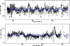 |
Fig. 1 Light curve of 28 Cyg observed with BTr (+) and UBr (°) in 2015 (top) and BTr in 2016 (bottom). Fitted constant-amplitude sine curves with frequencies 0.0508 c/d (2015) and 0.0496 c/d (2016) are overplotted in blue and trace the respective fΔ32 (≈ f3 − f2). JD = Julian Date. The zero points of the magnitude scales are arbitrary. It should be noted that the difference in magnitude scale between 2015 and 2016. Fifty-seven BeSS spectra were obtained between mJD 632 and 733 (see Figs. 19 and 20). |
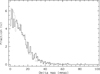 |
Fig. 2 Histogram of the magnitude differences between directly consecutive orbits (data points) of BRITE satellite BTr in 2015 (dotted line) and 2016 (solid line). |
 |
Fig. 3 B-band (crosses) and V -band (circles) fluxes (from SIMBAD) in annuli of 3 arcmin width around 28 Cyg. In both bands, the flux of 28 Cyg was set to unity. For BRITE observations in chopping (nodding) mode, the two positions of the point spread function (PSF) are contained in a window of 11 × 24 arcmin2. The PSF of SMEI was elongated, ~60 arcmin wide, and not box-car shaped. |
BRITE photometry of 28 Cyg with satellite BTr in 2015.
BRITE photometry of 28 Cyg with satellite BTr in 2016.
2.2 SolarMass Ejection Imager (SMEI)
The SMEI (Jackson et al. 2004; Howard et al. 2013) was a secondary payload on board the Coriolis spacecraft and tasked with monitoring space weather in the inner solar system. The signal recorded for this purpose was the Thomson-scattered solar light from ejected interplanetary electrons. Coriolis was launched in 2003 January into an orbit with a period of 101.6 min. The goal design lifetime was five years, but SMEI was eventually powered off only in 2012 September.
The SMEI delivered nearly 4π surface brightness measurements with three cameras with a field of view of 3 × 120 deg2 each and a basic angular sampling of 0.2° (0.1° for Camera 3). An inner zone of avoidance of 20° radius enabled some overlap between cameras. Camera 3 observed the region closest to the Sun and Camera 1 observed the zone farthest away from it. Point sources drifted through the combined field of view within ~1.5 min, and continuous 4-s exposures were obtained with one frame-transfer CCD per camera. The core unfiltered photometric passband ranged from 450 nm to 950 nm with a maximum near 700 nm. After an electronics failure in 2006, the temperature of Camera 3 rose, and its performance gradually degraded substantially.
The PSF of the deliberately defocussed cameras measures ~ 1° across, is highly asymmetric,and varies strongly over the path along which an object moved through the field of view (Hick et al. 2007). With its aperture of 1.76 cm2, SMEI could detect point sources of ~ 10m. Surface-brightness measurements with a precision of 0.1% required careful removal of stars brighter than ~ 6m from the images (Hick et al. 2007). In addition to direct and scattered light from discrete solar-system objects, the strongest background signal by far was the zodiacal light, which in some directions exceeded the signal from solar mass ejections by two orders of magnitude. It was removed by careful modelling. However, apart from any systematic issues, the stellar SMEI data inherited much photon noise from this background, to which the South Atlantic Anomaly made additional contributions. Radiation damage of the CCDs caused a loss in sensitivity of 1.6% per year and cosmetic problems.
Stellar fluxes (in SMEI magnitudes; Buffington et al. 2007) extracted by the UCSD pipeline (Hick et al. 2005) are available on the Web4. The only accompanying telemetry are observing dates and times so that it is not possible to analyse the observations separately for each camera. This has major repercussions as demonstrated below. So many years after the termination of the SMEI mission, the contact address provided at the UCSD SMEI Web site seems no longer actively supported. An example of observations with SMEI of relatively faint objects (novae) is available from Hounsell et al. (2010) who provide overall absolute errors around maximum (3.5−5.4 mag) of 0.01−0.02 mag.
The SIMBAD (Wenger et al. 2000) database lists 443 sources within 0.6° from 28 Cyg. Only relatively few have magnitudes in the R band, which is the best match of the sensitivity of SMEI. B and V fluxes for 323 and 314 sources, respectively, in SIMBAD account for 1.2 and 2.2 times as much flux as 28 Cyg alone. The distribution of these fluxes in annuli of 3 arcmin width is shown in Fig. 3.
The SMEI observations of 28 Cyg extended over 7.9 yr from February 4, 2003 to December 30, 2010 such that the nominal frequency resolution is ≤0.001 c/d. This dataset comprises a total of 34 335 data points. Since each data point results from one 101.6 min orbit, more than 80% of all orbits contributed, and the nominal Nyquist frequency is ~7.1 c/d. After removal of extreme outliers, the raw light curve (Fig. 4) revealed a strong need for correction for instrumental annual and other long-term variability. In addition, at some phases, the distribution of data points is bimodal, which is possibly due to the combination of data from different cameras. After pre-whitening for the annual variability by subtracting means in phase intervals of 0.01, a considerable annual pattern was still left because of season-dependent excess noise. These annual phase intervals were removed from the dataset, which thereby shrunk to 26 157 data points. Another 1184 presumed outliers were eliminated after its inspection.
Next, the spacing in time of the remaining 24 973 observations was studied. It can vary if the posted times correspond to the mean time of the 4-s exposures co-added for each orbit and the number of the latter varies because of rejected exposures. It was hypothesized that the best orbital data points are those that result from orbits without rejected measurements and that they can be identified by their spacing corresponding closely to the orbital period of 101.6 min. This selection reduced the number of data points to 23 708. Before this scheme was adopted, various others were explored, including permutations of the above steps. When the filtering according to the time elapsed between consecutive data points was performed at the beginning, it eliminated far more measurements than when done at the end. This demonstrates that the filtering of the annual light curve, which contains some subjective elements, has an objective background.
In addition to the annual variability (Fig. 4), SMEI data suffer instrumental variabilities faster than a year but slower than those measured in the BRITE observations of 28 Cyg (Sect. 3.1 and Table 5). Figure 5 depicts the full light curve with all corrections applied as described above. For the observations with SMEI of α Eri (B6 Ve), ζ Pup, and ζ Oph (O9.5 V), Goss et al. (2011), Howarth & Stevens (2014), and Howarth et al. (2014), respectively, used a boxcar filter of width 10 d to remove spurious non-stellar signals. In spite of the low accuracy of the individual SMEI measurements, their large number and long time span permitted these studies to detect significant variabilities at frequencies 0.7−7.2 c/d with amplitudes down to a few mmag. Experiments with filter widths between 6 d and 15 d showed that in the range above 0.5 c/d, where most of the BRITE frequencies occur, the results of the TSA are not very sensitive to the choice of the filter width, and it was decided to not apply any such filtering. The frequencies in common with both BRITE observing runs and their amplitudes are included in Table 5. All values therein are averages over the full range in time.
Figure 5 indicates the presence of some very slow regular variability. In the frequency spectrum, there is a strong, well-isolated peak at ff = 0.00471 c/d. The associated semi-amplitude is 16.7 mmag, i.e. far higher than any of the variations seen with BRITE. A sine fit with this frequency is overplotted in Fig. 5. Between phases 0.7 and 1.0, a similar bi-modal distribution of values as in the annual light curve (Fig. 4) is seen. The variability may, therefore, be due to an imperfect relative calibration of the cameras. For comparison, the SMEI data of some stars with similar positions in the sky ( λ Cyg [B5 V], υ Cyg [B2 Vne], QR Vul [B3 Ve]) were analysed. Very strong variability with 0.00411 c/d was found in υ Cyg and in QR Vul with 0.00473 c/d. Accordingly, f = 0.00471 c/d is not thought to be intrinisic to 28 Cyg.
The statistical properties of the SMEI data at their high-frequency end are illustrated by Fig. 6 which presents a histogram of the magnitude differences between immediately consecutive orbits. A comparison to the analogous Fig. 2 for BTr shows that the stellar-to-instrumental ratio of the contributions to these differences is smaller for SMEI, which has about the same orbital period as the BRITE satellites. This difference is owed to the systematics of the SMEI observations and the large noise from the bright background due to zodiacal and scattered solar light.
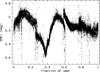 |
Fig. 4 Mean annual SMEI light curve of 28 Cyg (in SMEI magnitudes and clipped to the range shown). The bimodal distribution of values during some phases is probably the result of imperfect cross-calibration of the cameras. Fraction 0.0 corresponds to 1 January. |
SMEI photometry of 28 Cyg with satellite BTr in 2016.
Mean seasonal values of frequencies and semi-amplitudes in 28 Cyg.
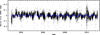 |
Fig. 5 SMEIlight curve of 28 Cyg after subtraction of the instrumental annual variation shown in Fig. 4 and after elimination of data from annual phases with elevated noise. In addition, some extreme outliers are clipped in this figure. No indication is visible of any photometric equivalent of the fading of the Hα emission between 2005/2007 and 2013 (Sect. 3.3). Overplotted in blue is a fitted sine curve with frequency 0.00471 c/d. |
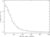 |
Fig. 6 Histogram of the magnitude differences between directly consecutive orbits (data points) of the SMEI data shown in Fig. 5. |
3 Analysis results
3.1 BRITE
3.1.1 Common periodic variations in 2015 and 2016
Figure 7 presents the frequency spectra of the BTr observations in 2015 and 2016 (Fig. 1). Beyond 3.5 c/d, no significant features can be found above the general noise floor. Obvious evidence for 1 c/d and related peaks cannot be seen either. A global pictorial overview of the variability of 28 Cyg as observed by BRITE is provided by the two time-frequency diagrams in Fig. 8.
In the BRITE frequency spectra, the three highest peaks above 0.5 c/d occur at f1 = 1.381 c/d, f2 = 1.545 c/d, and f3 = 1.597 c/d (here and in the following, all frequencies, etc. are from the combined analysis of the BTr observations in 2014, 2015, and 2016 unless explicitly identified otherwise). The strongest peak below 0.5 c/d appears at fΔ32 = 0.052 c/d. This slower variation is thought to be of initial relevance because the preparation of the raw data did not include any correction for slow variations. Growing evidence for the significance of fΔ32 will emerge during the course of this subsection. Despite the much shorter duration of the observations in 2014, fΔ32, f1, f2, and f3 were also clearly detected in this dataset alone.
Between the above frequencies, the following relation exists:
![Mathematical equation: \[ 0.0517\,\textrm{c/d} = f_{\Delta 32} \approx f_3 - f_2 = 0.0521\,\textrm{c/d}. \]](/articles/aa/full_html/2018/02/aa31187-17/aa31187-17-eq1.png)
The deviation from full equality amounts to 0.0004 c/d, which is of the order of the nominal single-season errors. Figure 1 presents the light curve associated with fΔ32 in 2015 and 2016.
In 2015, 28 Cyg did not undergo any obvious outburst signalling mass loss (Fig. 1). However, Fig. 9 suggests small enhancements of the photometric scatter during the maxima of the variability with fΔ32 = 0.051 c/d. The phase dependency of the scatter became very visible (Fig. 10) in 2016. The main contribution to this was made by the last three fΔ32 cycles in 2016, the amplitudes of which were up to an order of magnitude higher than in the five preceding cycles (Fig. 1). At the time of these brightenings, the light curve also exhibited interspersed short fadings well below the mean flux level.
Figure 7 shows also that the variability is clustered into three frequency groups with approximate ranges 0.1−0.5 c/d (g0), 1.0−1.7 c/d (g1 ), and 2.2−3.0 c/d (g2 ). The intervals between these groups are not perfectly devoid of power spikes. Contrary to g1, the frequencies in g2 common to 2015 and 2016 do not belong to the most prominent features of the group.
The large number of temporary frequencies prompted a search for frequency variations of f1, f2, f3, and other frequencies in single-season data. For each frequency, a sine curve was fitted to 40-d intervals of the dataset concerned, and this time window was shifted in steps of 1 d. No frequency appeared constant (Fig. 8). However, lower amplitude frequencies exhibited higher scatter, and the shorter time interval of 40 d implies larger uncertainties in general. Except for f1 to f3, which are discussed in the following, the results are, therefore, mostly inconclusive.
In both 2015 and 2016, f2 and f3 were modulated with their Δ frequency, fΔ32. The semi-amplitudes amounted to 0.005−0.007 c/d and f2 and f3 occurred nearly in anti-phase (Figs. 8 and 11). There is no signature of the large increase in amplitude of fΔ32 in the last two months of the 2016 observations. To test the robustness of the result, the time interval was varied between 20 d and 60 d in steps of 5 d. There was no elementary change, and the anti-phased modulation of f2 and f3 was confirmed in all cases. But the amplitude was much reduced at 60 d and f3 and f2 were no longer properly resolved towards 20 d because, in that case, the length of the interval corresponds to 1∕(f3 − f2).
A similar frequency modulation does not affect the nearby f1. The f1 frequency only suffered a major perturbation (Fig. 12) before the strong increase in amplitude of the fΔ32 variability around mJD = 610 (Fig. 1; mJD denotes a modified Julian Date: HJD − 2 457 000). However, during that phase of increased overall photometric amplitude, the amplitude of f1 displayed semi-regular large-amplitude variations with a cycle length comparable to, but clearly different from, that of fΔ32 (Fig. 13). There was similar activity at the end of the observations in 2015 (Fig. 13). By contrast, the amplitude variations off2 and f3 (Fig. 13) were an order of magnitude lower than those of f1. The difference between the stellar variabilities with f2 and f3 and the exophotospheric variability with f1 is very well visible in Fig. 8.
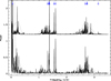 |
Fig. 7 BRITE frequency spectrum (in arbitrary units) of 28 Cyg. Top: frequency spectrum from 2015 for BTr and UBr satellites is shown; bottom: frequency spectrum from 2016 for BTr satellite is shown. Arrows denote the frequencies included in Table 5. The dashed lines represent the local sum of mean power and the × the scatter calculated after removal of the frequencies in Table 5. Between 3.5 c/d and the nominal Nyquist frequency near 7.2 c/d, there is virtually no power. Frequency groupings occur at the approximate ranges 0.1–0.5 c/d (g0 ), 1.0–1.7 c/d (g1), and 2.2–3.0 c/d (g2). |
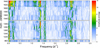 |
Fig. 8 Time vs. frequency diagrams for the BRITE red-filter photometry of 28 Cyg in 2014. The bottom panel shows a single time bin, the middle panel shows 2015, and the top panel represents 2016. The discrete Fourier transform frequency spectra werecalculated in 40-day intervals with a step of 1 d. The common amplitude scale appears on the right. Horizontal lines occur where data from different set-ups were stitched together. It should be noted that the diffuse appearance of fΔ32 (0.05 c/d) and f1 (1.38 c/d, the Štefl frequency) and the cyclic anti-phased variability of the two g modes f2 (1.54 c/d) and f3 (1.60 c/d). |
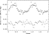 |
Fig. 9 Lightcurve from BTr 2015 from Fig. 1 binned to steps of 0.02 in phase of the 0.0508-c/d frequency (fΔ32). Zero points of flux and phase are arbitrary. For the same bins, the crosses indicate the scatter of the 2015 magnitudes in Fig. 1. It should be noted that the sign of the magnitude scale; the scatter is largest during light maxima. |
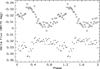 |
Fig. 10 Same as Fig. 9 except with BTr data from 2016 and fΔ32 = 0.0496 c/d. The offset in phase is arbitrary. |
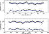 |
Fig. 11 Variability of f2 and f3 in 2015 (top) and 2016 (bottom). Frequencies were measured in a window of 40 d stepped by 1 d. The overplotted blue dotted lines are fitted sine curves with frequency 0.0508 c/d (2015) and 0.0496 c/d (2016), tracing the respective mean fΔ32. |
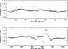 |
Fig. 12 Variability of f1 in 2015 (top) and 2016 (bottom). Frequencies were measured in a window of 40 d stepped by 1 d. |
 |
Fig. 13 Variability in amplitude of f1 (°), f2 (+), and f3 (×) in 2015 (top) and 2016 (bottom). Amplitudes were measured in windows of 10 d (f1 ) and 40 d (f2 and f3 ), stepped by 1d. |
3.1.2 Ephemeral variations
Figure 7 gives rise to the suspicion that ephemeral elements form a major part of the variability of 28 Cyg. Motivated by the strong changes around mJD 600, the 2016 data were split into two sets: mJD ≤ 600 and mJD > 600. The differences between their frequency spectra are stunning (Fig. 14). The extra features during the outburst may be mixtures of (i) combination frequencies; (ii) harmonics; (iii) side lobes due to the large-amplitude variation of fΔ32; (iv) circumstellar variations; and/or (v) stellar pulsations. Since none of these was detected in two or more independent datasets, their large number makes it next to impossible to identify the nature of any such single feature and their short lifespans prevent their characterization as periodic.
Temporarily enhanced visibility is not necessarily the same as increased amplitude or power. In very rapidly rotating stars, the angular parts of NRP eigenfunctions are described by a series of spherical harmonics (Lovekin & Deupree 2008). If the decomposition of eigenmodes into spherical harmonics changes during an outburst or brightening, this could also modify their visibility. In that case, such modes would not add to the cause of outbursts or brightenings. At the current level of analysis, only fΔ32 can be considered as causing mass loss.
The variability of Be stars is not erratic or even chaotic: the clear signature of low-order g-mode pulsations in high-resolution spectra (Rivinius et al. 2003) demonstrates coherent, and coherently varying, large-scale structures in the photosphere. Moreover, for several dozen spikes in the frequency spectrum the data were convolved with the corresponding frequencies, and in most cases the resulting light curve had an approximately sinusoidal shape.
Finally, the frequency spectra of the 2015/16 BTr data were searched for patterns by calculating histograms of nearest neighbour differences, frequency spectra (of the frequency spectra), and cross-correlation functions. The results were all negative, except for a possible overabundance of differences close to 0.01 c/d (e.g. 1.369 c/d – 1.360 c/d and 2.742 c/d – 2.732 c/d in Table 5; 1.369 and 2.742 c/d are harmonics). In the SMEI frequency spectrum, a feature exists at 0.00995 c/d; at 8.6 mmag, the amplitude is large. A similar light curve arises from the BTr observations in 2016.
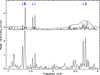 |
Fig. 14 Frequency spectra of the red 2016 BRITE observations before (top) and after (bottom) mJD 600 when a series of brightenings began (see Fig. 1). Power is given in arbitrary units. The arrows have the same meaning as in Fig. 7, and the full-season error curve (arbitrarily scaled) from Fig. 7 is also shown. In the top panel, frequency groups g1 (1.0–1.7 c/d)and g2 (2.2–3.0 c/d) are well separated. |
3.2 SolarMass Ejection Imager
The three main BRITE frequencies above 0.5 c/d also stand out in the SMEI data (Fig. 15). Peaks at fa = 1.3799 c/d, fb = 1.5447 c/d, and fc = 1.5970 c/d can be identified with f1, f2, and f3 (Table 5). That is, the mean frequencies in 2003−2010 (SMEI) and in 2014−2016 (BRITE) were the same. The long duration of the SMEI observations permits the constancy of the frequencies to be examined on shorter timescales. The results of single sine curves fitted to the data (Fig. 16: amplitudes; Fig. 17: frequencies) exhibit some commonalities of the amplitude variations of f2 and f3 whereas the behaviour of f1 is different and more pronounced. With a factor of ~3, the largest relative amplitude variation was associated with fΔ32.
In the SMEI observations, a similar relation exists between fa, fb, and fc as between f1, f2, and f3 with BRITE, i.e.
![Mathematical equation: \[ 0.05093\,\textrm{c/d} = f_{\Delta{cb}} \approx f_c - f_b = 0.05225\,\textrm{c/d}. \]](/articles/aa/full_html/2018/02/aa31187-17/aa31187-17-eq2.png)
The light curve after pre-whitening for 0.00471 c/d (Sect. 2.2) suggests that SMEI did not capture outbursts larger than 0.05 mag and longer than 100 d. This is in agreement with, but less stringent than, the BRITE observations (Sect. 3.1) and the findings of Percy & Bakos (2001). Even after this correction, no hint of a photometric counterpart of the fading of the Hα emission from 2005/2007 to 2013 (Sect. 3.3) is present.
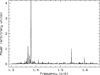 |
Fig. 15 Frequency spectrum (in arbitrary units) of the SMEI data in the region of the main BRITE frequencies above 0.5 c/d (fa: 1.381 c/d, fb: 1.545 c/d, and fc: 1.597 c/d). |
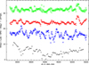 |
Fig. 16 Time-amplitude diagram for fΔ32 (black +), f1 (×), f2 (triangles), and f3 (°) in the SMEI data. The semi-amplitudes were derived from fits of single sine functions over windows of 100 d (fΔ32 : 300 d) stepped by 10 d (fΔ32: 30 d). From bottom to top, the curves are vertically shifted by 0, 10, 20, and 30 mmag, respectively. |
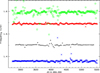 |
Fig. 17 Same as Fig. 16 except for time-frequency diagram. The frequency curve of fΔ32 ( ~0.05 c/d) was vertically shifted by 1.4 c/d. |
3.3 Spectroscopy
Tubbesing et al. (2000; see also Sect. 1) found two frequencies, ν1 = 1.54562 c/d and ν2 = 1.60033 c/d with radial velocity amplitudes of ~20 and ~10 km s−1, respectively. If corrected for a likely 1-c/yr alias, ν2 becomes 1.59726 c/d, and ν1 and ν2 can be perfectly identified with BRITE frequencies f2 = 1.5453 c/d and f3 = 1.5973 c/d, respectively. The associated line profile variability seems to be of the same ℓ = −m = 2 g-mode variety that is typical of classical Be stars (Rivinius et al. 2003). Accordingly, f2 and f3 are due to non-radial pulsation g modes.
As of February 2017, the BeSS database (Neiner et al. 2011) contained 118 wavelength-calibrated Hα line profiles contributed by more than a dozen amateurs between 1995 July and 2017 January; about half of these line profiles were contributed in 2016. Those observed since August 1997 were downloaded from the BeSS Web site. The equivalent widths derived from the line profiles are presented in Fig. 18. Like the photometry, the contemporaneous Hα spectroscopy conveys thepicture of 28 Cyg as one of the more quiet early-type Be stars. The Hα line emission was at a crudely constant high level through the end of 2002. From mid-2007 until early 2012 the Hα line emission was weak but again fairly constant. Thereafter, the line emission started to rise but did not reach the previous high level. The BRITE photometry started nearly three years after the onset of this partial recovery. During the BRITE observations the line emission stayed at some plateau with little variability. The overall timescale is at the long end of such cycles (e.g. Ghoreyshi et al. 2016).
There are no BeSS spectra from 1998 when Tubbesing et al. (2000) observed an outburst with HEROS. A single Hα profile 20 d before the amplitude maxima of fa, fb, and fc seen by SMEI (Sect. 3.2) is free of anomalies. Of the 62 BeSS spectra from 2016, 57 were obtained between mJD 630 and 740 in response to an alert when the online control of the BRITE observations had recognized the increased activity starting around mJD 600. The spectra were manually normalized with fitted splines, resampled from their original wavelength bins between 0.03 Å and 0.18 Å to a common 0.1 Å, and are plotted in Fig. 19.
The twoHα emission peaks are well, albeit not perfectly, approximated by Gaussians so that differential measurements from fitted Gaussians make sense. Figure 20 presents the variability in total equivalent width, peak-height (V∕R) ratio, and peak separation measured in the BeSS spectra; because of the inhomogeneous provenience of the observations only rough error estimates can be given. After mJD 650, there was a gentle increase by 25% in equivalent width. At about the same time, a fairly marked drop by more than 10% occurred in the peak separation. No attempt was made to search for repetitive variability on any timescale.
From 44 ground-based spectra Peters & Penrod (1988) derived an NRP period of 16.5 h (f: 1.45 c/d), which is a blend of f1 − f3, and found it co-phased with the equivalent width of C IV λλ 1548, 1551 in 17 R ≈ 10 000 spectra from the International Ultraviolet Explorer (IUE; Boggess et al. 1978). In 25 IUE spectra obtained within 56 h, Peters & Gies (2000) found a period of 0.646 ± 0.019 d (1.55 ± 0.05 c/d; i.e. very close to f2 = 1.545 c/d and still consistent with f3 = 1.600 c/d). Because the flux amplitude increased towards lower wavelengths, it was attributed to pulsational temperature variations. The C IV λ 1551 wind line exhibited correlated variability in equivalent width while the photospheric C III λ 124.7 nm and Si II λ 126.5 nm lines did not. However, Peters & Gies did not state whether the variability in line strength was above the escape velocity so that the relation to genuine mass loss is not clear.
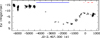 |
Fig. 18 Hα equivalentwidths in HEROS (Tubbesing et al. 2000, and unpublished; JD < 2 453 000) and BeSS (Neiner et al. 2011; JD > 2 453 000) spectra. Negative values mean net line emission. The 1σ scatter around JD 2452 000 is 0.5 Å; for BeSS errors see Fig. 20. The short red horizontal bars near the top right corner denote the BRITE observations. The long blue bar spans the SMEI observations. |
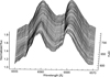 |
Fig. 19 Combination of 60 BeSS Hα profiles between mJD 589 and 733. The spectra were averaged over a window of 20 d stepped by 2 d. The spectral bin size is 0.1 Å. Only three spectra were obtained before mJD 633. The BRITE observations terminated on mJD 665. |
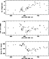 |
Fig. 20 Variability in total equivalent width (top; cf. Fig. 18) peak-height ratio (middle), and peak separation (bottom) of the violet and red Hα emission peaks in Fig.19. Estimated 1σ errors are 0.4 Å, 0.02, and 4 km s−1, respectively. |
3.4 Caveats and numerical limits
The analysis of the photometry of 28 Cyg reaches a fundamental mathematical limit: to measure a frequency f, a conservative rule of thumb is that the data should cover a time interval T ≥ 2/f. In the presence of noise, intervals larger by an order of magnitude are desirable. If the case of closely spaced power peaks, which, moreover, undergo independent variations, this minimal duration does often not suffice. The timescales of frequency and amplitude variations in 28 Cyg are comparable to this safe width of time windows. This touches upon the definition of a frequency.
Figure 8 illustrates the complexity of the variabilities, their variations in both frequency and power, in a single picture. For the numerous secondary frequencies (Sect. 3.1.2), error, and significance analyses attain a very limited meaning in the presence of the numerous interrelations.
The remainder of the paper only discusses frequencies f1, f2, f3, and fΔ32 (Table 5), all four of which were detected by BRITE in 2015 and 2016 (Sect. 3.1) and were confirmed with SMEI (Sect. 3.2). Moreover, f2 and f3 were spectroscopically discovered first. The maximal differences between the photometric values of these four frequencies are 0.0001, 0.0002, 0.0007, and 0.0013 c/d, respectively. Figure 8 suggests a frequency jitter above that level. Therefore, Table 5only contains frequencies detected in both BRITE datasets (from 2015 and 2016) and those agreeing to better than ~0.002 c/d. As becomes amply clear below, only very few of the many processes in 28 Cyg, if any, seem to be running on clocks with that precision. Moreover, the entries in Table 5 are seasonal averages. There are only 11 such seemingly persistent frequencies; these frequencies are indicated in Fig. 7.
A low-threshold search between 0 and 3.5 c/d at a sampling of 0.001 c/d found ≥60 frequency peaks in 2015 and ≥100 in 2016. For randomly distributed frequencies, the probability of chance coincidences within 0.002 c/d is, in that case, less than 6%. It is lower for the much fewer high-amplitude variabilities of Table 5. For a set of n lines in two independent observations (BRITE and SMEI), the single-frequency probability is raised to the nth power. The dashed lines in Fig. 7 indicate 3σ noise levels after subtraction of these variabilities. This rigorous approach does not take into account the large-amplitude variability of fΔ32, especially atthe end of the observations from 2016 (Fig. 1). Moreover, this approach attributes all other variability completely to stellar or instrumental noise. Such a classification system may be too crude for the variability of 28 Cyg (Sect. 3.1.2).
For reference, Kallinger et al. (2017) determined a total of 22 frequencies with errors between 0.9 and 92 × 10−5 c/d and amplitudes from 0.6 to 17 mmag from BRITE observations of the SPB star HD 201433. The SMEI and BRITE frequencies agreed at the 0.8 and 1.8σ level, respectively.In the longer SMEI observing sequences, nine rotationally split frequency pairs could be resolved.
Given the large PSFs of SMEI and BRITE, there is the risk that the main frequencies f1, f2, f3, and Δ32 are not intrinsicto 28 Cyg but are contributed by one or more other stars. Any such star would need to have fallen into the apertures of both SMEI and BRITE. The radius of a circle including the PSF at both nodding positions is ~12 arcmin. As of August 2017, the International Variable Star Index (Watson 2006) in VizieR (Ochsenbein et al. 2000) contains two variable stars within 15 arcmin from 28 Cyg. One (VSX J200906.4+365552) is an M5 V star that is listed as varying in R between 8.4 and 8.8 mag with unknown period. No period is known for the other star (VSX J201000.6+365111) as well and the stated R magnitude range is 11.8−12.4 mag.
In principle, this still leaves dozens of other objects as hypothetical real sources of the observed frequencies. However, since fΔ32 is the difference between f3 and f2, these three frequencies must be from one and the same star. Moreover, f2 and f3 were detected spectroscopically so that the common source of these three frequencies was in the aperture of the spectrograph. Only f1 could be from a second star; however, there are plausible reasons (Sect. 4.3) to identify it as the Štefl frequency of this Be star.
4 Discussion
4.1 Conceptual framework
Most Be stars undergo large-scale variations of their discs on timescales of years. Changes in total disc mass manifest themselves in varying Hα emission-line strengths and photometric amplitudes of several 0.1 mag (e.g. Keller et al. 2002). Evidence of more nearly periodic slow photometric variability in Be stars is still restricted to shorter timescales. Labadie-Bartz et al. (2017) present light curves of 11 Be stars with apparent periods >80 d. However, it is impossible to recognize any Be star by specific properties of this variability. Perhaps, this informational shallowness is the reason why the key to the understanding of the Be phenomenon has not been found therein.
Superimposed on this slow variability are outbursts. Their spectroscopic record is particularly rich and multifaceted for μ Cen, reaching from pulsationally triggered mass ejections (Rivinius et al. 1998a) via new matter settling in the circumstellar disc (Baade et al. 1988; Hanuschik et al. 1991)to gas moving towards the star at high velocity (Peters 1986). Neiner et al. (2002) also captured an outburst in spectra of ω Ori.
The build-up of line emission, i.e. a disc, as well as super-equatorial velocities associated with Štefl frequencies (Štefl et al. 1999)are evidence of star-disc mass transfer. There may also be numerous failed mass-loss events, during which matter is tossed up but does not reach an orbit as suggested by rapid variability in broadband polarimetry (Carciofi et al. 2007). Such cases are not easily diagnosed by spectroscopy but may still emit additional light or remove light from the line of sight, or both. Therefore, in the following we discuss brightenings and leave open from which level on they may be photometricequivalents of spectroscopic mass-loss events. Inspection of the light curve (Fig. 1) shows that 28 Cyg fairly regularly experiences brightenings with amplitudes well above the higher frequency variability floor.
For the interpretation of apparent exophotospheric photometric variability, the model calculations by Haubois et al. (2012) are used as the foundation. These models imply that at an inclination angle near 70° the photometric variability due to emission from variable amounts of near-stellar matter vanishes. On this basis, estimates of the inclination angle of 28 Cyg, 40° < i < 75° (Sect. 1), suggest that matter ejected into the equatorial plane produces extra emission that ought to reveal itself as brightenings (see also Fig. 21, top panel). However, the sensitivity may be small. In the wavelength region covered by BRITE Constellation, the matter involved is expected within about two radii of (one radius above) the stellar photosphere(Haubois et al. 2012). Photometry alone cannot determine whether this matter is already part of the disc, drifting towards it, or falling back to the star. It may form one large contiguous structure or be fractionated into numerous small blobs. Therefore, in the following we use the term exophotospheric emission regions (EERs) to allude to such situations.
The aspect-angle dependence may be different if matter were also lost at higher stellar latitudes (as also considered by Štefl et al. 2003a; Wisniewski et al. 2010). The ejecta may initially subtend an angle comparable to or smaller than the photosphere so that theyabsorb photospheric radiation as they quickly cool radiatively below the photospheric temperature. With time, the material spreads out, becomes much less dense, and partly reaches a Keplerian orbit. Most of this matter is not be seen projected on the stellar disc but, while close to the star, produce a brightening resulting from the reprocessing of stellar radiation.
To date, in the BRITE sample of Be stars, only η Cen has been examined (Paper I) in similar detail as 28 Cyg. In μ Cen (Paper I) strong emission from irregularly variable EERs seen at high inclination prevented detection of the stellar variability. The top-level variability of η Cen comprises the following: (i) two spectroscopically confirmed g modes; (ii) their Δ frequency with a much larger amplitude than the sum of the two g-mode amplitudes; and (iii) a so-called Štefl frequency that is exophotospheric in nature (cf. Sect. 4.5), ~10% slower than the g-modes, and has a very large amplitude. Paper I has argued that the Δ frequency modulates the star-to-disc mass transfer and the amplitude of the Štefl frequency traces the degree of orbital circularization of matter in the inner disc. A transient 0.5-c/d variability that Neiner et al. (2002) attribute to a cloud revolving ω CMa for a few orbits may be of a similar nature.
The structural similarity of the variabilities of η Cen and 28 Cyg is easily recognizable. 28 Cyg also features two g modes (f2 and f3 ); their Δ frequency fΔ32, whose average amplitude is not much smaller than those of f2 and f3 together; and f1, which is ~10% lower than f2 and f3 but has the largest mean amplitude (see Fig. 16). The structure of this section follows the structure of the variability. The stellar variability is evaluated in Sect. 4.3. Section 4.4 compiles the evidence that fΔ32 regulates the mass loss, and Sect. 4.5 examines f1 as a circumstellar Štefl frequency. The discussion begins with the slow irregular variability.
4.2 Slow and irregular variability
The clearest indicator of structural variations of Be discs is the violet-to-red ratio of emission peaks, V∕R. It is a robust estimator as it only requires a differential measurement. In high-inclination stars such as 28 Cyg, the large rotational peak separation makes V∕R variations easily detectable. This peak separation can be induced on very different timescales as global disc oscillations by the quadrupole moment of a rotationally distorted central star (Okazaki 1997), dynamically by any sufficiently massive and close companion (Štefl et al. 2007; Panoglou et al. 2018), radiatively by a hot companion (e.g. Peters et al. 2013; Mourard et al. 2015), and by non-axisymmetric mass injections. Also in this respect, 28 Cyg is at the far quiet end of the activity scale of early-type Be stars.
The persistent high degree of symmetry of the Hα line emission suggests that any undetected companion star is too ineffective in affecting the disc. Therefore, the explanation of the slow equivalent-width variations of the Hα profiles (Fig. 18), which leave no doubt that the disc around 28 Cyg was eroded for some years and was replenished around 2013, must be sought in a single-star context. Contrary to many years of ground-based photometric monitoring, Tubbesing et al. (2000) recorded a discrete mass-loss event in 1998, when the absolute value of the Hα equivalent width dropped by ~30%. The event lasted 10−15 d and was the only one observed in two seasons. The low level of disc activity is confirmed by the five-months BeSS snapshot (Figs. 19 and 20), during which no such event was observed (i.e. after the brightening starting around mJD600). The slow variability is probably due to oscillatory disc instabilities (Okazaki 1997).
The low variability in line emission is noteworthy because in the VDD model, without replenishment, Be discs are re-accreted within months to years (Carciofi et al. 2012; Vieira et al. 2017). Radiative ablation may accelerate this process (Kee et al. 2016a). Therefore, one might expect the Hα line emission to be fairly variable. The simplest resolution of this puzzle may consist of quasi-continuous star-to-disc mass transfer, which could also include small outbursts every couple of weeks.
4.3 The g modes f2 and f3 and other stellar variabilities
The most remarkable fact about the variability of 28 Cyg is the tight link, via fΔ32, between the two g modes with f2 and f3. Neither the reason nor the geometric depth of the combination is known. It could be just a linear superposition and merely appear as a coupling due to the extra emission from the mass ejections it causes, perhaps amplified by a non-linear response of the atmosphere to this slow and possibly non-adiabatic variability. There could also be non-linear mode coupling deep inside the star (Dziembowski 1982).
Two closely spaced frequencies also form part of an anchor variability pattern (cf. Sect. 4.1) in many other (early-type) Be stars. Examples include η Cen (Paper I), ψ Per, 25 ψ1 Ori (Baade et al. 2017a), 10 CMa, and 27 CMa (Baade et al. 2017b). However, in pole-on stars, the light curves are dominated by emission from varying amounts of near-stellar matter that blanket any underlying stellar variability. μ Cen (Paper I), κ CMa, and ω CMa (Baade et al. 2017b) are such cases. Therefore, the fraction of (early-type) Be stars with observed photometric Δ frequencies is always lower than the genuine incidence of Δ frequencies. If many Be stars exhibit large-amplitude Δ frequencies, the conditions for their formation should not be too special.
Among the frequencies investigated, f2 and f3 are the most stable (Figs. 8, 11, and 17; Table 5). However, these frequencies undergo a subtle modulation with fΔ32, i.e. their own difference. Not any less mysterious is that f2 and f3 vary in anti-phase (Figs. 8 and 11). This may harbour some hint as to how and where the coupling of these two NRP modes takes place. While it is still conceivable that the Δ frequency modulates the position of the layer where the waves associated with the g modes are reflectedand thereby modulates their apparent frequencies, it is not at all clear why two very closely spaced frequencies are affected in anti-phase.
Also the constancy in amplitude of f2 and f3 stands out above much of the rest (Figs. 8, 13, and 16). If the mass-loss modulation and apparent driving with fΔ32 (Sect. 4.4) were ultimately powered by these two g modes, one might not expect this. Comparison to ground-based studies shows that most of them found some blend of f1, f2, and f3 but could not resolve it. The implied apparent variability of the frequencies contributed to the notion prevailing at that time that the rapid variability of Be stars is mostly semi-regular. Thanks to BRITE and SMEI it is now clear that stellar variabilities can persist for decades (see also Paper I).
4.4 The variability associated with fΔ32: the brightening in 2016 and other mass-loss indicators
The difference frequency fΔ32 was not detected by ground-based observations; the value 0.09 c/d, reported by Ružić et al. (1994), is close to the first harmonic. The frequency fΔ32 is the only peak in group g0 that occurred in both 2015 and 2016. This frequency represents a variability in its own right as plain beat frequencies do not appear in power spectra. Figure 1 illustrates the difference well. The rise in amplitude of fΔ32 at the end of the observations in 2016 sets in rather suddenly and after an extended period of quiescence. Similarly rapid rises and drops in the amplitude of Δ frequencies have also been seen in 25 ψ1 Ori (Baade et al. 2017b). A simple beating of two frequencies looks different.
During its maximum, the amplitude of fΔ32 reaches a PTV value of 100 mmag. This is well outside the domain of non-radial pulsations in other B-type stars and exceeds the (time-independent; see Fig. 13) amplitude sum of its parent frequencies f2 and f3 by a factor of 4−5. Other stars with Δ amplitudes above the sum of the parent amplitudes include η Cen (Paper I), 10 CMa, and 25 ψ1 Ori (Baade et al. 2017b). Moreover, the variability with fΔ32 is highly non-sinusoidal and the range above the inflection points of the light curve is much larger than that below (Fig. 1). This asymmetry and the large amplitude can be understood as near-circumstellar matter emitting extra light (Haubois et al. 2012; Baade et al. 2016). Such large-amplitude asymmetries have also been observed by BRITE Constellation in 25 ψ1 Ori (Baade et al. 2017b). Because of the EER effects, it is not possible to infer the real photospheric amplitude associated with fΔ32 and the above comparison of Δ-frequency amplitude and parent g-mode amplitudes has no energetic meaning.
Figure 1 reveals another important detail. In the fΔ32 cycle around mJD 630, several measurements appear up to ~100 mmag below the upper envelope of the light curve. These measurements reach well below the mean brightness so that there is a temporary deficit of light. These fadings should not be instrumental because both UBr and BTr independently recorded a similar, slightly weaker, event around mJD 198 (Fig. 1). The reality of this dimming is undoubtable. But the absence of simultaneous observations at all other times makes it impossible to assess the reality of any of the other, mostly much sparser, groups of bright and faint points. However, Figs. 9 and 10 point to increased scatter around extrema of the fΔ32 light curve.
Comparable rapid switching between increased and attenuated brightness during phases of maximal Δ amplitude has been observed by BRITE in 25 ψ1 Ori (Baade et al. 2017b). This star has a spectral type and v sin i similar to 28Cyg such that it is also viewed from a similar perspective. One possible interpretation (cf. Sect. 4.1) is, therefore,that ejecta span some range in stellar latitude. The emission by the lifted-up matter is permanent (but not constant) whereas the only temporary removal of light implies strong variability in the amount of matter along the line of sight to the photosphere. This corroborates the conclusion that at the end of the BRITE observations in 2016 28 Cyg suffered a (small) series of mass ejections. That is, these brightenings probably were real outbursts.
With this behaviour of 28 Cyg (and 25 ψ1 Ori) there are three ways in which a Δ frequency can sculpt mass loss from Be stars:
- 1)
Spectroscopy of μ Cen (Rivinius et al. 1998a) has shown that major enhancements of the Hα line emissionhappen every time when the vectorial sum of at least two out of three specific NRP modes exceeds a threshold in amplitude.
- 2)
In η Cen (Paper I), the mass loss is basically permanent as is suggested by the continuous presence of the Štefl frequency in emission lines, which seems to be the response by the disc to mass transfer. The latter is continually modulated by fΔ32 with minor apparently stochastic deviations superimposed.
- 3)
The same may be at work in 28 Cyg but at a lower level (Fig. 9, Sect. 4.5). Much more prominent are single events spaced with the Δ period. But the series of such events starts suddenly and, by inference from 25 ψ1 Ori, also declines quickly; the observations of 28 Cyg in 2016 were terminated before the end of the active phase because the Sun was too close. This confirms the report by Tubbesing et al. (2000) that they saw only one Hα line-emission outburst and could rule out repetitions with fΔ32 = 0.05 c/d during their 100-d and 65-d observing windows.
It remains to be seen whether these three categories are genuine or the artefact of incomplete temporal sampling. There is no explanation of the timing of the brightenings in 28 Cyg. They may involve a third clock (in addition to f2 and f3).
4.5 The nature of f1 as a Štefl frequency and other circumstellar variabilities
Paper I called the high-amplitude 1.56-c/d frequency of η Cen a Štefl frequency after the discoverer of this kind of variability (Štefl et al. 1998). In η Cen, the Štefl frequency was spectroscopically detected (Rivinius et al. 2003). Typical Štefl frequencies occur during outbursts, are best seen in emission lines and absorption lines formed high in the atmosphere, and – for unknown or accidental reasons – appear to have values ~10% below the main spectroscopic frequency. Condensed to the capabilities of photometry, this is a good initial description of f1 in 28 Cyg.
In η Cen, both amplitude and frequency of the Štefl frequency are strongly variable and appear modulated with the Δ frequency (Paper I). In 28 Cyg, the variations are also large but there is no regularity in the frequency, only a major perturbation just before the series of brightenings in 2016 (Figs. 8 and 12). This large frequency jitter is also reminiscent of Achernar, in which Goss et al. (2011) meticulously documented phase shifts of one of the two detected frequencies.
The maxima of the brightenings are roughly matched by strong amplitude maxima of f1 (compare Figs. 1, 8, and 13). This is compatible with the spectroscopically established notion of Paper I. When an outburst or brightening occurs, the distribution of matter in the inner disc is not yet homogeneous (Baade et al. 1988; Hanuschik et al. 1991). The level of inhomogeneity reveals itself by the amplitude of the Štefl frequency. As in η Cen and other Be stars observed by BRITE, f1 is embedded in a frequency group (g1; Figs. 7, 14, and 15) the strength of which is crudely related to that of the f1. In 28 Cyg, a fair part of the neighbourhood of f1 changes during a major brightening (Fig. 14). Both observations probably strengthen the notion that these apparent companion frequencies are circumstellar. On all these the grounds, the classification of f1 as the Štefl frequency of 28 Cyg appears safe.
At 9 M⊙, the model ofHaubois et al. (2012) should be a good match to a B2 star such as 28 Cyg (cf. Harmanec 1988). At the assumed typical fractional critical rotation rate of 80% (Frémat et al. 2005; Meilland et al. 2012; Rivinius et al. 2013) its equatorial radius is increased from 5.7 R⊙ to 6.5 R⊙. The orbital radius of matter circling this star with the Štefl frequency, 1.4 c/d, amounts to 6.9 R⊙. A comparison of the two radii not only supports the exophotospheric interpretation of the Štefl frequency but is also consistent with the model prediction that, at optical wavelengths, the emission from exophotospheric matter arises from a region measuring less than about two equatorial radii.
In spite of all these details, the net effect of the brightenings in 2016 remains uncertain. The event reported by Tubbesing et al. (2000) impacted a fair part of the disc. But the cadence of the spectroscopy did not trace accompanying star-disc connections. The BRITE photometry has the necessary sampling but cannot equally clearly distinguish between photospheric and exophotospheric variability. Photometry by BRITE and HEROS spectroscopy can be reconciled if the 1998 drop in Hα emission strength was caused by a short increase of the continuum flux similar to that recorded by BRITE in 2016. This would also be in good agreement with the models of Haubois et al. (2012).
The contemporaneous BeSS spectroscopy (Fig. 20) exhibits no direct counterpart of the photometric brightenings. A most sensitive indicator could be the wings of the Hα line emission. The effects of the high orbital velocity of, and Thomson scattering by, inner disc matter should both strengthen the wings (Baade 1986), but only in dense discs. At the time of the BeSS spectroscopy in 2016 the disc of 28 Cyg was only moderately developed. This probably explains why enhanced Hα wings were not detected (Fig. 19) in the wake of the brightening around mJD 630.
Figure 20 could be read as follows: at some moment, fresh matter was injected into the disc. With the help of viscosity, part of it drifted outwards but most of it lost angular momentum and fell back to the star. Because the disc is optically thick in Hα, the equivalent width did not change immediately after the outburst but only started to increase when the outwards drifting matter reached a domain that was not optically thick before. Since this region is farther away from the star and the disc is Keplerian, the separation of the emission peaks decreased.
This description is consistent with VDD hydrodynamic simulations coupled with radiative transfer calculations (Haubois et al. 2012). Figure 21 illustrates a periodic model (see Fig. 7 of Haubois et al. 2012), which alternates between one year of disc build-up at a fixed disc-feeding rate with one year of disc dissipation when the mass loss is shut off. At t = 8 yr, the outburst begins, replenishing the remnant of the disc from the previous two-year cycle with fresh material. Initially the line equivalent width drops slightly, as a result of the increased EER continuum emission. But then this line equivalent width raises steadily and continues to grow past the cessation of the disc feeding at t = 9 yr owing to the quick decrease in the EER continuum emission. As observed in 28 Cyg (Fig. 20), the peak separation anti-correlates with line emission, but this is no longer true during disc dissipation.
Although f1 exhibits large-amplitude variations, it never disappears completely. If Štefl frequencies are indeed close tracers of star-to-disc mass transfer, the implication is that this mass transfer was variable but permanent during the BRITE observations of 28 Cyg. Such a continuous, albeit variable, process may make larger contributions to the regular disc replenishment needed to overcome the demolishing effect of the viscosity than outbursts. This is another important commonality with η Cen (Paper I). It also seems supported by the persistence, for five months, of fairly strong wings of the not-so-strong Hα line emission(Fig. 19). Even in a late-type Be star, whose disc may additionally be truncated by a companion star, the Hα line emission forms over many stellar radii (Klement et al. 2015). Therefore, the inner disc volume, when well filled, acts as a buffer that is insensitive to minor variations of the mass inflow.
The amplitude of f1 was also increased at the end of the observations in 2015 (Figs. 8 and 13) when there was no hint of a major brightening (Fig. 1). This might indicate that the steady mass-loss component can also lead to inhomogeneous mass distributions close to the star (unless due to intrinsic local instabilities), or the outburst was not strong enough to develop a disc.
Unless winds of Be stars originate from the circumstellar discs (Rivinius et al. 2013), in which case a direct link to pulsation is not expected, it would be interesting to repeat the simultaneous UV and optical spectroscopy by Peters & Gies (2000) to identify which of f1, f2, and f3, if any, correlates with UV flux and wind. To date, in no Be star, including 28 Cyg, has precision photometry or spectroscopy found mass loss clearly modulated with the frequency of a single NRP mode. Instead, timescales 20−50 times longer (occurring as Δ frequencies) have been inferred. It would be useful to extend UV observations to this range and also to check for the distribution of the variability between sub- and super-escape velocities. The sampling should permit detection of the circumstellar f1.
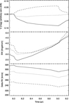 |
Fig. 21 Temporal evolution of the V -band brightness (top), Hα line equivalent width (middle), and peak separation (bottom) computed with the periodic model of Haubois et al. (2012, their Fig. 7) consisting of a series of one-year disc build-up phases followed by one-year dissipation phases. Solid, dotted, and dashed lines represent inclination angles 80°, 70°, and 60°, respectively. It should be noted that the difference in sign between the V magnitude changes at 80° and 60°. The outburst begins at t = 8 yr and ends at t= 9 yr. |
5 Conclusions and outlook
In the photometric variability of early-type Be stars some incipient commonalities emerge as a set of frequencies that follow a common pattern whose numerical values form the specific fingerprint of every star. The top-level variability of 28 Cygni is structurally the same as that of the very similar star η Cen (Paper I):
(i) Most frequencies are concentrated in groups (Fig. 7).
(ii) Four frequencies dominate the short- and medium-term variability. They fall into three different categories:
(iia) Two spectroscopically confirmed g modes (f2 and f3, Tubbesing et al. 2000).
(iib) One Štefl frequency (f1), which originates from the star-disc transition zone and is about 10% lower in value than f2 and f3. This frequency may occasionally become undetectable, and it can drastically increase around brightenings but does not contribute to the brightenings (Fig. 13). Its frequency is much less stable than the frequencies of the g modes (Figs. 8 and 12). But its average value is roughly constant at all times.
(iic) One Δ frequency (fΔ32) of the two g modes. It has the largest amplitude. During amplitude maxima, star-to-disc mass loss seems increased as indicated by the enhancement of the Štefl variability of emission lines in η Cen (Paper I; for 28 Cyg, see Figs. 1, 9, and 10). This process may also be persistently modulated with the Δ frequency.
At this level, η Cen and 28 Cyg only differ in the numerical values of the parameters quantifying the frequencies and their amplitudes. Both stars also share the long-term persistence of their basic variability patterns, including considerable amplitude variations especially of f1 and fΔ32.
The existence of a second star, such as η Cen, lends considerable support to the description of the variability given in Paper I. An inner “engine” clocked by the g modes and powered by the Δ variability lifts matter above the photosphere. In the inner disc, a viscosity-ruled outer engine sorts the matter delivered to it into two categories, namely super- and sub-Keplerian specific angular momentum. Part of this process is observed as Štefl frequency, the amplitude of which increases with the total amount of inner-disc matter and its deviation from circular symmetry. It is not yet possible to guess whether or not η Cen and 28 Cyg are representative of a significant fraction of all early-type Be stars.
Walker et al. (2005, MOST), Huat et al. (2009, CoRoT), Neiner et al. (2012, CoRoT), Kurtz et al. (2015, Kepler), and others have argued that the myriads of frequencies in Be stars are due to pulsations. With so much support, this conclusion is not to be dismissed lightly. However, Papers I and II of this series have suggested on several grounds that a circumstellar origin may be a fairly reasonable alternative for a good part of this variability. The coming and going of many features in the frequency spectrum also of 28 Cyg (Sect. 3.1.2 and Fig. 8) may also point at the Štefl frequency as the tip of the iceberg.
Therefore, it makes sense to search for the key to the understanding of the Be phenomenon in the small set of anchor frequencies instead of transient variations. Only for these frequencies is there any plausible direct observed link to mass loss (Figs. 1, 9, and 10). Ultimately, this requires that undulations of the short-term variability can also explain disc life cycles of up to a decade inferred from the Hα emission-line strength (taken as a proxy of the total amount of matter in the circumstellar disc). In 28 Cyg, anchor frequencies have persisted for several decades, which is long enough to allow such frequencies to contribute to the explanation.
The simplest extrapolation in timescale to nearly a decade (0.1 c/yr) would be a combination of modes with Δ frequencies of order 0.1 c/yr. However, viscosity does not let single big outbursts every 10 yr create photometric high states lasting several years. In the VDD paradigm, a photometric high state of a disc could result from outbursts with a frequency and effectiveness sufficient to sustain a massive disc. The lowest level would be formed by mini-outbursts with single Δ frequencies. A second clock could come into play for outbursts perhaps associated with the brightening in 28 Cyg around mJD 630. At least a third level would be required to regulate the first two processes and cause cycles of a few years length. The example of the brightening around mJD 630 illustrates that the amplitude amplification can be a highly non-linear process, either in true NRP amplitudes or their effect on mass loss or both.
One way of achieving slow clocking could be “hierarchical” Δ frequencies, i.e. combinations of Δ frequencies. In 28 Cyg, they could be fΔ32 and, if real, 0.00995 c/d (Sect. 3.1.2). In their most basic form, these frequencies might explain seemingly particularly simple cases as depicted in Fig. 5 of Keller et al. (2002) in which long-lasting bright states cyclically repeat on two similar timescales of order 500−1000 d.
Irrespective of how several NRP wave patterns combine to Δ frequencies, it seems plausible that for best coupling efficiency their angular structures must be the same, i.e. they should agree in their ℓ and m indices. In μ Cen (Rivinius et al. 1998b) and 28 Cyg (Tubbesing et al. 2000) the available spectroscopic evidence supports this expectation. The work of Rivinius et al. (2003) has furthermore demonstrated that ℓ = − m = 2 modes dominate the spectral variability of many Be stars. If equality of the mode indices is a requirement for mass-loss-modulating difference frequencies, this could be an important filter, meaning that no two arbitrary NRP modes can combine to cause mass loss. Indications of mass lift-ups occurring over some range in stellar latitude may place first constraints on the pulsational velocity field (ℓ and m). However, spectroscopic searches for Δ frequencies could be more effective in determining the geometry of the variability. It would be desirable to learn from models whether energy leakage from pulsations to mass loss can establish another effective filter of the NRP mode spectrum.
A robust distinction between stellar and circumstellar phenomena is critical for the identification of frequencies for asteroseismology. High-cadence long-term space photometry has the potential of achieving this. For the understanding of the Be phenomenon at large, it is comforting that with the VDD model a tool is available that permits observed circumstellar variabilities to be cast into coherent sequences of dynamical states.
Acknowledgements
The authors thank the BRITE operations staff for their untiring efforts to deliver data of the quality that enabled this investigation. We are also very grateful to the many amateur astronomers who, in response to a specific request, took numerous Hα spectra and shared them through BeSS. This research has made use of the SIMBAD database, operated at CDS, Strasbourg, France. This research hasmade use of NASA’s Astrophysics Data System. This work has made use of the BeSS database, operated at LESIA, Observatoire de Meudon, France: http://basebe.obspm.fr. A.C.C. acknowledges the support from CNPq (grant 307594/2015-7) and FAPESP (grant 2015/17967-7). D.P. acknowledges financial support from Conselho Nacional de Desenvolvimento Científico e Tecnológico (CNPq-MCTIC Brazil; grant 300235/2017-8). M.R.G. acknowledges the support from CAPES PROEX Programa Astronomia. G.H. thanks the Polish NCN for support (grant 2015/18/A/ST9/00578). A.F.J.M. is grateful for financial aid from NSERC (Canada) and FRQNT (Quebec). A.Pi. acknowledges support from the Polish NCN grant No. 2016/21/B/ST9/01126. A.Po. acknowledges support through NCN grant No. 2016/21/D/ST9/00656. G.A.W. acknowledges Discovery Grant support from the Natural Sciences and Engineering Research Council (NSERC) of Canada. The Polish contribution to the BRITE project is supported by Polish Ministry of Science and Higher Education, and the Polish National Science Center (NCN, grant 2011/01/M/ST9/05914).
References
- Ando, H. 1986, A&A, 163, 97 [NASA ADS] [Google Scholar]
- Baade, D. 1986, Bull. Inf. Etoiles Be, 13, 5 [NASA ADS] [Google Scholar]
- Baade, D., Dachs, J., van de Weygaert, R., & Steeman, F. 1988, A&A, 198, 211 [NASA ADS] [Google Scholar]
- Baade, D., Rivinius, T., Pigulski, A., et al. 2016, A&A, 588, A56 (Paper I) [NASA ADS] [CrossRef] [EDP Sciences] [Google Scholar]
- Baade, D., Rivinius, T., Pigulski, A., Carciofi, A., & BEST Collaboration 2017a, in ASP Conf. Ser. 508, eds. A. Miroshnichenko, S. Zharikov, D. Kor cáková, & M. Wolf, 93 [Google Scholar]
- Baade, D., Rivinius, T., Pigulski, A., et al. 2017b, in Second BRITE-Constellation Science Conf.: Small Satellites Big–Science, Proc. of the Polish Astronomical Society, 5, 196 [Google Scholar]
- Boggess, A., Carr, F. A., Evans, D. C., et al. 1978, Nature, 275, 372 [NASA ADS] [CrossRef] [Google Scholar]
- Boley, P. A., Linz, H., van Boekel, R., et al. 2013, A&A, 558, A24 [NASA ADS] [CrossRef] [EDP Sciences] [Google Scholar]
- Bossi, M., Guerrero, G., & Zanin, F. 1993, A&A, 269, 343 [NASA ADS] [Google Scholar]
- Buffington, A., Morrill, J. S., Hick, P. P., et al. 2007, in Solar Physics and Space Weather Instrumentation II, Proc. SPIE, 6689, 66890 [CrossRef] [Google Scholar]
- Carciofi, A. C., & Bjorkman, J. E. 2006, ApJ, 639, 1081 [NASA ADS] [CrossRef] [Google Scholar]
- Carciofi, A. C., Magalhães, A. M., Leister, N. V., Bjorkman, J. E., & Levenhagen, R. S. 2007, ApJ, 671, L49 [NASA ADS] [CrossRef] [Google Scholar]
- Carciofi, A. C., Bjorkman, J. E., Otero, S. A., et al. 2012, ApJ, 744, L15 [NASA ADS] [CrossRef] [Google Scholar]
- Ducati, J. R. 2002, VizieR Online Data Catalog: II/237 [Google Scholar]
- Dziembowski, W. 1982, Acta Astron., 32, 147 [NASA ADS] [Google Scholar]
- Frémat, Y., Zorec, J., Hubert, A.-M., & Floquet, M. 2005, A&A, 440, 305 [NASA ADS] [CrossRef] [EDP Sciences] [Google Scholar]
- Ghoreyshi, M. R., Carciofi, A. C., Bjorkman, J., et al. 2016, in Bright Emissaries: Be Stars as Messengers of Star-Disk Physics, eds. T. A. A. Sigut, & C. E. Jones, ASP Conf. Ser., 506, 315 [NASA ADS] [Google Scholar]
- Gies, D. R., & Percy, J. R. 1977, AJ, 82, 166 [NASA ADS] [CrossRef] [Google Scholar]
- Goss, K. J. F., Karoff, C., Chaplin, W. J., Elsworth, Y., & Stevens, I. R. 2011, MNRAS, 411, 162 [NASA ADS] [CrossRef] [Google Scholar]
- Hahula, M. E., & Gies, D. R. 1994, in Pulsation; Rotation; and Mass Loss in Early-Type Stars, eds. L. A. Balona, H. F. Henrichs, & J. M. Le Contel, IAU Symp., 162, 100 [NASA ADS] [Google Scholar]
- Hanuschik, R. W., Baudzus, M., Thimm, G., & Dachs, J. 1991, in European Southern Observatory Conference and Workshop Proc. 36, ed. D. Baade, 185 [Google Scholar]
- Harmanec, P. 1983, Hvar Observatory Bulletin, 7, 55 [Google Scholar]
- Harmanec, P. 1988, Bull. Astron. Inst. Czechoslovakia, 39, 329 [Google Scholar]
- Haubois, X., Carciofi, A. C., Rivinius, T., Okazaki, A. T., & Bjorkman, J. E. 2012, ApJ, 756, 156 [NASA ADS] [CrossRef] [Google Scholar]
- Hick, P., Buffington, A., & Jackson, B. V. 2005, in Solar Physics and Space Weather Instrumentation, eds. S. Fineschi, & R. A. Viereck, Proc. SPIE, 5901, 340 [NASA ADS] [Google Scholar]
- Hick, P., Buffington, A., & Jackson, B. V. 2007, in Solar Physics and Space Weather Instrumentation II, Proc. SPIE, 6689, 66890 [Google Scholar]
- Hounsell, R., Bode, M. F., Hick, P. P., et al. 2010, ApJ, 724, 480 [NASA ADS] [CrossRef] [EDP Sciences] [Google Scholar]
- Howard, T. A., Bisi, M. M., Buffington, A., et al. 2013, Space Sci. Rev., 180, 1 [NASA ADS] [CrossRef] [Google Scholar]
- Howarth, I. D., & Stevens, I. R. 2014, MNRAS, 445, 2878 [NASA ADS] [CrossRef] [Google Scholar]
- Howarth, I. D., Goss, K. J. F., Stevens, I. R., Chaplin, W. J., & Elsworth, Y. 2014, MNRAS, 440, 1674 [NASA ADS] [CrossRef] [Google Scholar]
- Huat, A.-L., Hubert, A.-M., Baudin, F., et al. 2009, A&A, 506, 95 [NASA ADS] [CrossRef] [EDP Sciences] [Google Scholar]
- Jackson, B. V., Buffington, A., Hick, P. P., et al. 2004, Sol. Phys., 225, 177 [Google Scholar]
- Jiménez-Vicente, J., Mediavilla, E., Muñoz, J. A., & Kochanek, C. S. 2012, ApJ, 751, 106 [NASA ADS] [CrossRef] [Google Scholar]
- Kallinger, T., Weiss, W. W., Beck, P. G., et al. 2017, A&A, 603, A13 [NASA ADS] [CrossRef] [EDP Sciences] [Google Scholar]
- Kee, N. D., Owocki, S., & Sundqvist, J. O. 2016a, MNRAS, 458, 2323 [NASA ADS] [CrossRef] [Google Scholar]
- Kee, N. D., Owocki, S., Townsend, R., & Müller, H.-R. 2016b, in Bright Emissaries: Be Stars as Messengers of Star-Disk Physics, eds. T. A. A. Sigut, & C. E. Jones, ASP Conf. Ser., 506, 47 [NASA ADS] [Google Scholar]
- Keller, S. C., Bessell, M. S., Cook, K. H., Geha, M., & Syphers, D. 2002, AJ, 124, 2039 [NASA ADS] [CrossRef] [Google Scholar]
- Klement, R., Carciofi, A. C., Rivinius, T., et al. 2015, A&A, 584, A85 [NASA ADS] [CrossRef] [EDP Sciences] [Google Scholar]
- Krtička J. 2014, A&A, 564, A70 [Google Scholar]
- Kurtz, D. W., Shibahashi, H., Murphy, S. J., Bedding, T. R., & Bowman, D. M. 2015, MNRAS, 450, 3015 [NASA ADS] [CrossRef] [Google Scholar]
- Labadie-Bartz, J., Pepper, J., McSwain, M. V., et al. 2017, AJ, 153, 252 [Google Scholar]
- Lee, U., Osaki, Y., & Saio, H. 1991, MNRAS, 250, 432 [NASA ADS] [CrossRef] [Google Scholar]
- Lovekin, C. C., & Deupree, R. G. 2008, ApJ, 679, 1499 [NASA ADS] [CrossRef] [Google Scholar]
- Meilland, A., Millour, F., Kanaan, S., et al. 2012, A&A, 538, A110 [NASA ADS] [CrossRef] [EDP Sciences] [Google Scholar]
- Mourard, D., Monnier, J. D., Meilland, A., et al. 2015, A&A, 577, A51 [NASA ADS] [CrossRef] [EDP Sciences] [Google Scholar]
- Neiner, C., Hubert, A.-M., Floquet, M., et al. 2002, A&A, 388, 899 [NASA ADS] [CrossRef] [EDP Sciences] [Google Scholar]
- Neiner, C., de Batz, B., Cochard, F., et al. 2011, AJ, 142, 149 [Google Scholar]
- Neiner, C., Floquet, M., Samadi, R., et al. 2012, A&A, 546, A47 [NASA ADS] [CrossRef] [EDP Sciences] [Google Scholar]
- Ochsenbein, F., Bauer, P., & Marcout, J. 2000, A&AS, 143, 23 [NASA ADS] [CrossRef] [EDP Sciences] [Google Scholar]
- Okazaki, A. T. 1997, A&A, 318, 548 [NASA ADS] [Google Scholar]
- Okazaki, A. T. 2007, in Active OB-Stars: Laboratories for Stellare and Circumstellar Physics, eds. A. T. Okazaki, S. P. Owocki, & S. Stefl, ASP Conf. Ser., 361, 230 [NASA ADS] [Google Scholar]
- Okazaki, A. T., Bate, M. R., Ogilvie, G. I., & Pringle, J. E. 2002, MNRAS, 337, 967 [NASA ADS] [CrossRef] [Google Scholar]
- Pablo, H., Whittaker, G. N., Popowicz, A., et al. 2016, PASP, 128, 125001 [NASA ADS] [CrossRef] [Google Scholar]
- Panoglou, D., Faes, D. M., Carciofi, A. C., et al. 2018, MNRAS, 473, 3039 [NASA ADS] [CrossRef] [Google Scholar]
- Pavlovski, K., & Ruzic, Z. 1990, A&A, 236, 393 [NASA ADS] [Google Scholar]
- Pavlovski, K., Harmanec, P., Bozic, H., et al. 1997, A&AS, 125, 75 [NASA ADS] [CrossRef] [EDP Sciences] [Google Scholar]
- Percy, J. R., & Bakos, A. G. 2001, PASP, 113, 748 [NASA ADS] [CrossRef] [Google Scholar]
- Percy, J. R., & Lane, M. C. 1977, AJ, 82, 353 [NASA ADS] [CrossRef] [Google Scholar]
- Pereira-Santaella, M., Diamond-Stanic, A. M., Alonso-Herrero, A., & Rieke, G. H. 2010, ApJ, 725, 2270 [NASA ADS] [CrossRef] [Google Scholar]
- Peters, G. J. 1986, ApJ, 301, L61 [NASA ADS] [CrossRef] [Google Scholar]
- Peters, G. J., & Gies, D. R. 2000, in IAU Colloq. 175: The Be Phenomenon in Early-Type Stars, eds. M. A. Smith, H. F. Henrichs, & J. Fabregat, ASP Conf. Ser., 214, 375 [NASA ADS] [Google Scholar]
- Peters, G. J., & Penrod, G. D. 1988, in ESA SP, 281, 117 [Google Scholar]
- Peters, G. J., Pewett, T. D., Gies, D. R., Touhami, Y. N., & Grundstrom, E. D. 2013, ApJ, 765, 2 [NASA ADS] [CrossRef] [Google Scholar]
- Popowicz, A. 2016, in Space Telescopes and Instrumentation 2016: Optical, Infrared, and Millimeter Wave, Proc. SPIE, 9904, 99041 [NASA ADS] [Google Scholar]
- Popowicz, A., Pigulski, A., Bernacki, K., et al. 2017, A&A, 605, A26 [NASA ADS] [CrossRef] [EDP Sciences] [Google Scholar]
- Prinja, R. K. 1989, MNRAS, 241, 721 [NASA ADS] [CrossRef] [Google Scholar]
- Rivinius, T., Baade, D., Š tefl, S., et al. 1998a, in A Half Century of Stellar Pulsation Interpretation, eds. P. A. Bradley, & J. A. Guzik, ASP Conf. Ser., 135, 343 [NASA ADS] [Google Scholar]
- Rivinius, T., Baade, D., Štefl, S., et al. 1998b, A&A, 336, 177 [NASA ADS] [Google Scholar]
- Rivinius, T., Baade, D., Štefl, S., & Maintz, M. 2001, A&A, 379, 257 [NASA ADS] [CrossRef] [EDP Sciences] [Google Scholar]
- Rivinius, T., Baade, D., & Štefl S. 2003, A&A, 411, 229 [NASA ADS] [CrossRef] [EDP Sciences] [Google Scholar]
- Rivinius, T., Štefl, S., & Baade, D. 2006, A&A, 459, 137 [NASA ADS] [CrossRef] [EDP Sciences] [Google Scholar]
- Rivinius, T., Carciofi, A. C., & Martayan, C. 2013, A&ARv, 21, 69 [Google Scholar]
- Rivinius, T., Baade, D., & Carciofi, A. C. 2016, A&A, 593, A106 (Paper II) [NASA ADS] [CrossRef] [EDP Sciences] [Google Scholar]
- Rivinius, T., Baade, D., & Carciofi, A. C. 2017, in Second BRITE-Constellation Science Conf.: Small satellites Big–Science, Proc. of the Polish Astronomical Society, 5, 188 [Google Scholar]
- Ruzić, Z., Vujnović, V., Pavlovski, K., et al. 1994, in Pulsation; Rotation; and Mass Loss in Early-Type Stars, eds. L. A. Balona, H. F. Henrichs, & J. M. Le Contel, IAU Symp., 162, 102 [NASA ADS] [Google Scholar]
- Sigut, T. A. A., & Jones, C. E. 2007, ApJ, 668, 481 [NASA ADS] [CrossRef] [Google Scholar]
- Slettebak, A. 1982, ApJS, 50, 55 [NASA ADS] [CrossRef] [Google Scholar]
- Spear, G. G., Mills, J. Jr., & Snedden, S. A. 1981, PASP, 93, 460 [NASA ADS] [CrossRef] [Google Scholar]
- Stee, P., & Bittar, J. 2001, A&A, 367, 532 [NASA ADS] [CrossRef] [EDP Sciences] [Google Scholar]
- Štefl, S., Baade, D., Rivinius, T., et al. 1998, in A Half Century of Stellar Pulsation Interpretation, eds. P. A. Bradley, & J. A. Guzik, ASPConf. Ser., 135, 348 [Google Scholar]
- Štefl, S., Aerts, C., & Balona, L. A. 1999, MNRAS, 305, 505 [NASA ADS] [CrossRef] [Google Scholar]
- Štefl, S., Baade, D., Rivinius, T., et al. 2003a, A&A, 402, 253 [NASA ADS] [CrossRef] [EDP Sciences] [Google Scholar]
- Štefl, S., Baade, D., Rivinius, T., et al. 2003b, A&A, 411, 167 [NASA ADS] [CrossRef] [EDP Sciences] [Google Scholar]
- Štefl, S., Okazaki, A. T., Rivinius, T., & Baade, D. 2007, in Active OB-Stars: Laboratories for Stellare and Circumstellar Physics, eds. A. T. Okazaki, S. P. Owocki, & S. Stefl, ASP Conf. Ser., 361, 274 [NASA ADS] [Google Scholar]
- Tubbesing, S., Rivinius, T., Wolf, B., & Kaufer, A. 2000, in IAU Colloq. 175,The Be Phenomenon in Early-Type Stars, eds. M. A. Smith, H. F. Henrichs, & J. Fabregat, ASP Conf. Ser., 214, 232 [NASA ADS] [Google Scholar]
- Vieira, R. G., Carciofi, A. C., & Bjorkman, J. E. 2015, MNRAS, 454, 2107 [NASA ADS] [CrossRef] [Google Scholar]
- Vieira, R. G., Carciofi, A. C., Bjorkman, J. E., et al. 2017, MNRAS, 464, 3071 [NASA ADS] [CrossRef] [Google Scholar]
- Wade, G. A., Petit, V., Grunhut, J. H., Neiner, C., & MiMeS Collaboration 2016, in Bright Emissaries: Be Stars as Messengers of Star-Disk Physics, eds. T. A. A. Sigut, & C. E. Jones, ASP Conf. Ser., 506, 207 [NASA ADS] [Google Scholar]
- Walker, G. A. H., Kuschnig, R., Matthews, J. M., et al. 2005, ApJ, 635, L77 [NASA ADS] [CrossRef] [Google Scholar]
- Watson, C. L. 2006, Soc. Astron. Sci. Ann. Symp., 25, 47 [NASA ADS] [Google Scholar]
- Weiss, W. W., Rucinski, S. M., Moffat, A. F. J., et al. 2014, PASP, 126, 573 [NASA ADS] [CrossRef] [Google Scholar]
- Wenger, M., Ochsenbein, F., Egret, D., et al. 2000, A&AS, 143, 9 [NASA ADS] [CrossRef] [EDP Sciences] [Google Scholar]
- Wisniewski, J. P., Draper, Z. H., Bjorkman, K. S., et al. 2010, ApJ, 709, 1306 [NASA ADS] [CrossRef] [Google Scholar]
- Zhao, M., Gies, D., Monnier, J. D., et al. 2008, ApJ, 684, L95 [NASA ADS] [CrossRef] [Google Scholar]
All Tables
All Figures
|
Fig. 1 Light curve of 28 Cyg observed with BTr (+) and UBr (°) in 2015 (top) and BTr in 2016 (bottom). Fitted constant-amplitude sine curves with frequencies 0.0508 c/d (2015) and 0.0496 c/d (2016) are overplotted in blue and trace the respective fΔ32 (≈ f3 − f2). JD = Julian Date. The zero points of the magnitude scales are arbitrary. It should be noted that the difference in magnitude scale between 2015 and 2016. Fifty-seven BeSS spectra were obtained between mJD 632 and 733 (see Figs. 19 and 20). |
| In the text | |
|
Fig. 2 Histogram of the magnitude differences between directly consecutive orbits (data points) of BRITE satellite BTr in 2015 (dotted line) and 2016 (solid line). |
| In the text | |
|
Fig. 3 B-band (crosses) and V -band (circles) fluxes (from SIMBAD) in annuli of 3 arcmin width around 28 Cyg. In both bands, the flux of 28 Cyg was set to unity. For BRITE observations in chopping (nodding) mode, the two positions of the point spread function (PSF) are contained in a window of 11 × 24 arcmin2. The PSF of SMEI was elongated, ~60 arcmin wide, and not box-car shaped. |
| In the text | |
|
Fig. 4 Mean annual SMEI light curve of 28 Cyg (in SMEI magnitudes and clipped to the range shown). The bimodal distribution of values during some phases is probably the result of imperfect cross-calibration of the cameras. Fraction 0.0 corresponds to 1 January. |
| In the text | |
|
Fig. 5 SMEIlight curve of 28 Cyg after subtraction of the instrumental annual variation shown in Fig. 4 and after elimination of data from annual phases with elevated noise. In addition, some extreme outliers are clipped in this figure. No indication is visible of any photometric equivalent of the fading of the Hα emission between 2005/2007 and 2013 (Sect. 3.3). Overplotted in blue is a fitted sine curve with frequency 0.00471 c/d. |
| In the text | |
|
Fig. 6 Histogram of the magnitude differences between directly consecutive orbits (data points) of the SMEI data shown in Fig. 5. |
| In the text | |
|
Fig. 7 BRITE frequency spectrum (in arbitrary units) of 28 Cyg. Top: frequency spectrum from 2015 for BTr and UBr satellites is shown; bottom: frequency spectrum from 2016 for BTr satellite is shown. Arrows denote the frequencies included in Table 5. The dashed lines represent the local sum of mean power and the × the scatter calculated after removal of the frequencies in Table 5. Between 3.5 c/d and the nominal Nyquist frequency near 7.2 c/d, there is virtually no power. Frequency groupings occur at the approximate ranges 0.1–0.5 c/d (g0 ), 1.0–1.7 c/d (g1), and 2.2–3.0 c/d (g2). |
| In the text | |
|
Fig. 8 Time vs. frequency diagrams for the BRITE red-filter photometry of 28 Cyg in 2014. The bottom panel shows a single time bin, the middle panel shows 2015, and the top panel represents 2016. The discrete Fourier transform frequency spectra werecalculated in 40-day intervals with a step of 1 d. The common amplitude scale appears on the right. Horizontal lines occur where data from different set-ups were stitched together. It should be noted that the diffuse appearance of fΔ32 (0.05 c/d) and f1 (1.38 c/d, the Štefl frequency) and the cyclic anti-phased variability of the two g modes f2 (1.54 c/d) and f3 (1.60 c/d). |
| In the text | |
|
Fig. 9 Lightcurve from BTr 2015 from Fig. 1 binned to steps of 0.02 in phase of the 0.0508-c/d frequency (fΔ32). Zero points of flux and phase are arbitrary. For the same bins, the crosses indicate the scatter of the 2015 magnitudes in Fig. 1. It should be noted that the sign of the magnitude scale; the scatter is largest during light maxima. |
| In the text | |
|
Fig. 10 Same as Fig. 9 except with BTr data from 2016 and fΔ32 = 0.0496 c/d. The offset in phase is arbitrary. |
| In the text | |
|
Fig. 11 Variability of f2 and f3 in 2015 (top) and 2016 (bottom). Frequencies were measured in a window of 40 d stepped by 1 d. The overplotted blue dotted lines are fitted sine curves with frequency 0.0508 c/d (2015) and 0.0496 c/d (2016), tracing the respective mean fΔ32. |
| In the text | |
|
Fig. 12 Variability of f1 in 2015 (top) and 2016 (bottom). Frequencies were measured in a window of 40 d stepped by 1 d. |
| In the text | |
|
Fig. 13 Variability in amplitude of f1 (°), f2 (+), and f3 (×) in 2015 (top) and 2016 (bottom). Amplitudes were measured in windows of 10 d (f1 ) and 40 d (f2 and f3 ), stepped by 1d. |
| In the text | |
|
Fig. 14 Frequency spectra of the red 2016 BRITE observations before (top) and after (bottom) mJD 600 when a series of brightenings began (see Fig. 1). Power is given in arbitrary units. The arrows have the same meaning as in Fig. 7, and the full-season error curve (arbitrarily scaled) from Fig. 7 is also shown. In the top panel, frequency groups g1 (1.0–1.7 c/d)and g2 (2.2–3.0 c/d) are well separated. |
| In the text | |
|
Fig. 15 Frequency spectrum (in arbitrary units) of the SMEI data in the region of the main BRITE frequencies above 0.5 c/d (fa: 1.381 c/d, fb: 1.545 c/d, and fc: 1.597 c/d). |
| In the text | |
|
Fig. 16 Time-amplitude diagram for fΔ32 (black +), f1 (×), f2 (triangles), and f3 (°) in the SMEI data. The semi-amplitudes were derived from fits of single sine functions over windows of 100 d (fΔ32 : 300 d) stepped by 10 d (fΔ32: 30 d). From bottom to top, the curves are vertically shifted by 0, 10, 20, and 30 mmag, respectively. |
| In the text | |
|
Fig. 17 Same as Fig. 16 except for time-frequency diagram. The frequency curve of fΔ32 ( ~0.05 c/d) was vertically shifted by 1.4 c/d. |
| In the text | |
|
Fig. 18 Hα equivalentwidths in HEROS (Tubbesing et al. 2000, and unpublished; JD < 2 453 000) and BeSS (Neiner et al. 2011; JD > 2 453 000) spectra. Negative values mean net line emission. The 1σ scatter around JD 2452 000 is 0.5 Å; for BeSS errors see Fig. 20. The short red horizontal bars near the top right corner denote the BRITE observations. The long blue bar spans the SMEI observations. |
| In the text | |
|
Fig. 19 Combination of 60 BeSS Hα profiles between mJD 589 and 733. The spectra were averaged over a window of 20 d stepped by 2 d. The spectral bin size is 0.1 Å. Only three spectra were obtained before mJD 633. The BRITE observations terminated on mJD 665. |
| In the text | |
|
Fig. 20 Variability in total equivalent width (top; cf. Fig. 18) peak-height ratio (middle), and peak separation (bottom) of the violet and red Hα emission peaks in Fig.19. Estimated 1σ errors are 0.4 Å, 0.02, and 4 km s−1, respectively. |
| In the text | |
|
Fig. 21 Temporal evolution of the V -band brightness (top), Hα line equivalent width (middle), and peak separation (bottom) computed with the periodic model of Haubois et al. (2012, their Fig. 7) consisting of a series of one-year disc build-up phases followed by one-year dissipation phases. Solid, dotted, and dashed lines represent inclination angles 80°, 70°, and 60°, respectively. It should be noted that the difference in sign between the V magnitude changes at 80° and 60°. The outburst begins at t = 8 yr and ends at t= 9 yr. |
| In the text | |
Current usage metrics show cumulative count of Article Views (full-text article views including HTML views, PDF and ePub downloads, according to the available data) and Abstracts Views on Vision4Press platform.
Data correspond to usage on the plateform after 2015. The current usage metrics is available 48-96 hours after online publication and is updated daily on week days.
Initial download of the metrics may take a while.