| Issue |
A&A
Volume 609, January 2018
|
|
|---|---|---|
| Article Number | A18 | |
| Number of page(s) | 7 | |
| Section | The Sun | |
| DOI | https://doi.org/10.1051/0004-6361/201731827 | |
| Published online | 22 December 2017 | |
Guided flows in coronal magnetic flux tubes⋆
1 INAF–Osservatorio Astronomico di Palermo, Piazza del Parlamento 1, 90134 Palermo, Italy
e-mail: This email address is being protected from spambots. You need JavaScript enabled to view it.
2 Dipartimento di Fisica & Chimica, Università di Palermo, Piazza del Parlamento 1, 90134 Palermo, Italy
3 Smithsonian Astrophysical Observatory, 60 Garden Street, MS 58, Cambridge, MA 02138, USA
Received: 25 August 2017
Accepted: 27 October 2017
Abstract
Context. There is evidence that coronal plasma flows break down into fragments and become laminar.
Aims. We investigate this effect by modelling flows confined along magnetic channels.
Methods. We consider a full magnetohydrodynamic (MHD) model of a solar atmosphere box with a dipole magnetic field. We compare the propagation of a cylindrical flow perfectly aligned with the field to that of another flow with a slight misalignment. We assume a flow speed of 200 km s-1 and an ambient magnetic field of 30 G.
Results. We find that although the aligned flow maintains its cylindrical symmetry while it travels along the magnetic tube, the misaligned one is rapidly squashed on one side, becoming laminar and eventually fragmented because of the interaction and back-reaction of the magnetic field. This model could explain an observation made by the Atmospheric Imaging Assembly on board the Solar Dynamics Observatory of erupted fragments that fall back onto the solar surface as thin and elongated strands and end up in a hedge-like configuration.
Conclusions. The initial alignment of plasma flow plays an important role in determining the possible laminar structure and fragmentation of flows while they travel along magnetic channels.
Key words: magnetohydrodynamics (MHD) / Sun: activity / Sun: corona
Movies are available in electronic form at http://www.aanda.org
© ESO, 2017
1. Introduction
Plasma flows are ubiquitous in the solar corona. They can be generated by many different processes characterized by the interaction between the strong and complex magnetic field of the corona and its plasma. The interaction can be relatively weak – leading to confined flows, e.g. spicules (Beckers 1968; de Pontieu et al. 2007), siphon flows (Rueedi et al. 1992; Brekke et al. 1997; Mariska & Dowdy 1992; Winebarger et al. 2001, 2002; Teriaca et al. 2004), and coronal rain (Parker 1953; Field 1965; Antolin & Rouppe van der Voort 2012) – or it can be strong – leading to violent ejection of plasma outside of the Sun in coronal mass ejections (CMEs, Chen 2011; Webb & Howard 2012).
In an impressive eruption event that occurred on 7 June 2011, the ejected material fell back along parabolic trajectories and impacted the solar surface (Carlyle et al. 2014; van Driel-Gesztelyi et al. 2014; Innes et al. 2012), producing brightenings (Reale et al. 2013). In this case, the dynamics were strongly influenced by the intensity and the complexity of the magnetic field close to the impact region. In particular, impacts where the magnetic field is weak brighten because of the shock heating of their outer shells (Reale et al. 2013, 2014), other plasma blobs are channelled by a strong magnetic field, and the shocks brighten the whole channel ahead (Petralia et al. 2016). Petralia et al. (2017) show that the misalignment between the velocity of the blobs and the magnetic field lines determines a significant disruption of the blobs.
The misalignment between plasma flows and the ambient magnetic field can therefore be important. Magnetohydrodynamic (MHD) modelling of the solar chromosphere up to the corona has shown that chromospheric flows are not always aligned with the magnetic field (Martínez-Sykora et al. 2016). As we show, there is evidence for this misalignment from the observations as well.
In this work, we address specifically the possible role of the initial field alignment or misalignment of a persistent outflow ejected in a magnetized atmosphere. Our approach is to model flows which are pushed upward from the chromosphere along closed magnetic flux tubes in the corona by means of 3D MHD simulations able to capture the relevant physics behind the process and to take into account other important effects, such as the natural expansion of the magnetic channel cross section with the height and its effect on the dynamics, or possible transversal motions of the flow (e.g. Petralia et al. 2016). We first show an observed sample case of laminar fragmented flow in Sect. 2. The model is described in Sect. 3. The simulations and the results are presented in Sect. 4, and we discuss them in Sect. 5.
2. Observed sample case
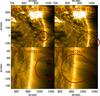 |
Fig. 1 Evolution of falling material observed in the 171 Å band of SDO/AIA on 4 November 2015 at the labelled times (see the associated movie). |
After a solar eruption on 4 November 2015, SDO/AIA observed dense fragments falling back onto the solar surface. During the fall they elongated, spread, and then impacted the solar surface in a row in a hedge-like configuration, as shown in Fig. 1 and in the associated movie. This evolution might not appear obvious, but our present model may explain it. The fragments are observed in absorption and this allows us to estimate their density and temperature according to the method in Landi & Reale (2013). We obtain a density of ~1.5 × 1010 cm-3 and a temperature of ~4 × 10⁴ K. We also estimate the impact velocity perpendicular to the solar surface by assuming a parabolic motion. We measure the vertical distance (H) covered from the apex of the trajectory to the impact region and we obtained a final velocity of  km s-1, where g⊙ is the solar gravity. The observed evolution and destiny of the erupted fragments suggest that this is an example of an outflow that is initially not perfectly aligned with the magnetic field coming out of the solar surface, as illustrated in the following sections.
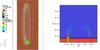 |
Fig. 2 Initial model conditions for the misaligned flow. Rendering of the density (units of 2 × 1010 cm-3, logarithmic scale) viewed from above, i.e. the line of sight is aligned with the Z-axis (left panel), and from the side, i.e. on an XZ plane (right panel), in the computational domain (axis in units of 109 cm). A bundle of magnetic field lines (in gauss) is also shown. |
3. Model
We use the model presented in Petralia et al. (2016) and the numerical code PLUTO (Mignone et al. 2012) to describe the dynamics of a persistent flow injected upwards and confined inside a closed coronal magnetic flux tube. This is very similar to the dynamics of siphon flows. We consider two slightly different flow directions, one perfectly aligned to the field and the other slightly inclined with respect to the field lines. In the following, we will call the former “Aligned Flow” and the latter “Misaligned Flow”.
The ambient atmosphere is made by a stratified million-degree corona linked to a much denser chromosphere through a steep transition region. The corona is a hydrostatic atmosphere (Rosner et al. 1978; Serio et al. 1981) that extends upwards for 1010 cm. The chromosphere below is hydrostatic and isothermal at 104 K with a density at the base of ~1016 cm-3. The atmosphere is made plane-parallel along the vertical direction (Z).
The closed magnetic loop is obtained by setting a dipole magnetic field centred on and parallel to the solar surface (XY). The field intensity is ~30 G at the top of the chromosphere and rapidly decreases with the height (Fig. 2). The field confines the flow, but can be perturbed by it; indeed, the ratio between the ram pressure carried by the flow and the magnetic pressure is  at the top of the transition region. This ratio may be expected in an active region loop.
We consider the same ambient atmosphere as the “Dense Model” described in Petralia et al. (2016), that – combined with the field intensity – gives an Alfvén speed of ~2000 km s-1 at the top of the chromosphere close to the footpoint of the loop.
Figures 2 and 3 show our initial conditions. The flow is injected upwards from a localized area of the chromosphere and is continuously fed from the lower domain boundary, i.e. the injection is set as a boundary condition inside the flow area at the base of the chromosphere. The flow area is a circle with a radius RF = 2 × 108 cm. The flow has been present since the beginning of the model inside the domain above the lower boundary, as shown in Fig. 2, in the shape of a cylinder with a vertical length of LF = 109 cm. Its initial density and temperature are uniformly 3 × 1010 cm-3 and 4 × 10⁴ K, respectively. Since the thickness of the chromosphere is ≈7 × 108 cm, the tip of the jet protrudes into the corona.
The misaligned flow is injected at a distance X = 1.3 × 109 cm from the left boundary where the magnetic field lines rapidly curve and leads to a misalignment of the flow. The flow propagates in the quasi semi-circular flux tube that has a distance between the footpoints of ~4 × 109 cm and a height of 2.5 × 109 cm above the chromosphere.
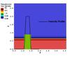 |
Fig. 3 Same as Fig. 2 (right), but including the initial spatial profile of the velocity across the flow (black line) in units of 100 km s-1. |
As shown in Fig. 3, the velocity of the flow is uniform along the Z direction vZ = 200 km s-1 inside an inner circular area with radius R = 108 cm, and then linearly decreases to zero in an outer shell to the cylinder boundary R = 2 × 108 cm. This initial velocity is such that the flow has enough kinetic energy to reach and surpass the apex of the closed flux tube.
The aligned flow is injected instead at a smaller distance X = 0.9 × 109 cm from the left boundary, where the magnetic field lines are nearly open and thus vertical because closer to the magnetic pole and aligned with the vertical direction of the flow. This flow will travel to a much greater height along the flux tube (Fig. 3).
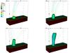 |
Fig. 4 Simulation of the aligned flow. Rendering of the density (109 cm-3, logarithmic scale) at times t = 0, 20, 40, 100 s, where a bundle of magnetic field lines are shown (see the associated movie). |
The computational box is three-dimensional and Cartesian (X, Y, Z) and extends over 6 × 109 cm in the X direction, 1 × 109 cm in the Y direction, and 6 × 109 cm in the Z direction, which is perpendicular to the solar surface. The mesh of the 3D domain is adaptively refined to strong gradients of density. The roughest level has a total of 120 × 20 × 120 cells and it is refined up to three levels. Each level refines locally the mesh by a factor of 2, giving a cell size of ~60 km at the highest level of refinement. The geometry of the system is symmetric with respect to the Y = 0 plane, allowing us to simulate only half of the domain.
Therefore, at the Y = 0 plane boundary we impose reflecting conditions. At all the other boundaries the magnetic field is fixed. For the other physical variables, we impose outflow conditions at all boundaries except for the plane at the base of the chromosphere, i.e. at Z = 0. There, we have fixed values and zero velocity outside the flow area, and inflow condition inside the flow area, i.e. a fixed velocity with the same radial dependence as in the inner domain. Thus, the flow velocity at the boundary is also constant in time.
4. Results
4.1. Aligned flow
Figure 4 shows four snapshots of the evolution of the aligned flow. The flow propagates in a flux tube that is almost vertical at the injection site; therefore, it reaches a maximum height and eventually falls back onto the chromosphere.
The jet is initially uniform along the vertical direction, while the surrounding atmosphere is not. This means that the flow is not in pressure equilibrium with the ambient atmosphere; in particular, below the transition region (not shown in Fig. 4, see Fig. 5), at the lower boundary, the ambient chromosphere is very dense and the thermal pressure (pchrom> 104 dyn cm-2) is much higher than inside the flow (pflow ~ 10-1 dyn cm-2, pmag ~ 4 × 10² dyn cm-2). Therefore, at its origin, both the flow and the magnetic field inside it are rapidly squeezed by the outside pressure and the flow is de facto quenched after ~40 s of evolution. This might not be entirely realistic, although we expect that such rapid flows do not have enough time to reach pressure equilibrium while crossing the chromosphere. However, the initial supply is large enough to sustain the flow along the magnetic channel. This also applies to the case of misaligned flow described in Sect. 4.2.
Since the initial speed of the flow (vflow = 200 km s-1) exceeds the (isothermal) sound speed ( km s-1, with T ~ 8 × 10⁵ K), a shock front is generated. This is a slow-mode shock that moves ahead of the flow (see the pale blue cocoon in Fig. 5) along the magnetic field lines. Its initial compression ratio of the density is ρpost−shock/ρpre−shock ≈ 2.8, and the temperature grows by ~15% in the post-shock. The overall propagation is similar to that shown in Petralia et al. (2016).
The flow moves upwards without deviating from the initial direction and as a uniform cylinder. Since its thermal pressure is much greater than that of the surrounding corona, the flow expands at the tip and pushes apart the magnetic field where it propagates. However, since the magnetic field is tightly anchored at the footpoint of the flux tube, its expansion rapidly stops (with Alfvénic time scales) and the tension constrains the flow. As a result, a thin shell of overdense plasma forms all around the head of the flow, as shown in Figs. 5 and 6, which is progressively smoothed out. Overall, the flow keeps its uniformity and cylindrical symmetry while it propagates upwards.
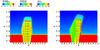 |
Fig. 5 Density maps (units of 109 cm-3, logarithmic scale) on an XZ cross section across the centre of the domain at time t = 20 s, for the aligned (left) and for the misaligned flow (right). A bundle of magnetic field lines (in gauss) and the velocity field (km s-1) are also shown. |
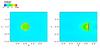 |
Fig. 6 Density maps (units of 109 cm-3, logarithmic scale) on an XY cross section at Z = 2 × 109 cm and at time t = 100 s, for the aligned (left) and for the misaligned flow (right). |
4.2. Misaligned flow
Figure 7 shows some snapshots of the evolution of the misaligned flow (see also the associated movie). Although overall the flow still moves along the magnetic flux tube, the detailed evolution is very different from that of the strictly aligned flow. Again a shock (not visible) is generated and moves ahead of the flow along the tube and the injection is quenched from below. Both the compression ratio of density (~1.7) and the temperature increase (~10%) are smaller than in the aligned case. This is mainly due to the misalignment, as only the component of the velocity along the field lines contributes. The shock propagates in the hot ambient corona and is potentially visible in the EUV band. Although this is the case closer to the observation described in Sect. 2, we are actually unable to detect the shock in the data, probably because it is not dense enough to stand out in the thick bright solar limb.
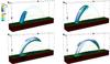 |
Fig. 7 Snapshots from our simulation of a misaligned flow: Rendering of the density (109 cm-3, logarithmic scale) at times t = 80, 160, 320, 480 s where a bundle of magnetic field lines (in gauss) is shown (see the associated movie). |
Since the magnetic flux tube is closed on the chromosphere, the shock hits the other footpoint, at t = 260 s (when the flow has just crossed the apex of the magnetic channel). Its average speed is therefore vsh ~ 220 km s-1.
The bulk plasma motion visible in Fig. 7 and the associated movie has a small component perpendicular to the magnetic field, which has been present since the beginning. Although the plasma is forced to move along the field lines, its misaligned momentum distorts the field above the chromosphere. The flux tube still expands, but the expansion is no longer symmetric.
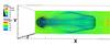 |
Fig. 8 Simulation of the misaligned flow: top view of the density rendering (109 cm-3, logarithmic scale) at time t = 320 s where a bundle of magnetic field lines (in gauss) is shown. |
In turn, the deformed field deviates the flow in the direction of the tube curvature, already at t = 20 s, as we can see in Fig. 5. Since the dense plasma is forced to flow in a direction different from the initial one, its structure becomes asymmetric. It converges and thus is squashed on the side of the curvature, where the magnetic field offers more resistance to deformation. It expands more freely on the other side.
The interplay between the magnetic back-effects (magnetic pressure and tension) and the upward push of the flow is very strong until the flow reaches the apex of the magnetic channel at t ~ 200 s. After this time, the magnetic field starts to relax to the initial configuration, while the flow falls on the other side of the magnetic channel. The relaxation of the field lines acts as a press that flattens the flux tube and deforms the flow inside it even more. The flow expands laterally at t ~ 320 s (Fig. 8). The relaxation of the field is untidy and frays the flow; as the flow moves along the tube, it splits and becomes highly substructured at the end of the evolution at t ~ 480 s (Fig. 7).
Overall, we observe an initially cylindrical and uniform flow becoming laminar and filamentary, basically because of the initial misalignment of its direction to the field lines.
Figures 5 and 6 compare density maps in different cross sections at early times and emphasize the difference between the symmetric structure of the aligned flow and the strong bending of the misaligned flow. Figure 6 shows how the thin dense shell all around the aligned flow is squashed on the side of the curved field in the misaligned flow and eventually determines the laminar structure of the flow.
5. Discussion and conclusions
In this work, we analyse the dynamics of a continuous flow perfectly or not perfectly aligned to the field lines of a magnetic channel anchored to the solar surface by means of a 3D MHD model analogous to that presented in Petralia et al. (2016).
Summarizing, we find that the aligned flow travels mostly unperturbed along the magnetic channel, except for some expansion at the tip and for the formation of a dense outer shell. If instead the field lines are strongly curved and the flow is forced to change its direction to follow the magnetic channel, the evolution is significantly different. Because of the stiffness of the field, the flow is squashed to the side of the curved lines and converts into a dense laminar flow, strikingly different from the symmetric dense shell found when the alignment is perfect. As the flow travels through regions of weaker field, it causes some deformation of the field and its untidy back-reaction makes the flow split. The propagation has been monitored until the flow hits the chromosphere at the other side of the closed channel.
We expect that the result can change somewhat for different conditions in the model, but we are unable to quantify the change without a relevant exploration of the parameter space. For instance, we might expect that a weaker field and/or a more tenuous ambient atmosphere should make the flow expansion easier and perhaps smooth down the dense shell of the aligned flow. A faster outflow in the curved loop should determine a stronger deformation of the field and we might expect an even larger back-reaction and flow splitting.
The transformation of the initially cylindrical, symmetric, and uniform flow into a strongly laminar and substructured flow might explain the puzzling evidence of hedge-like downfalls observed with SDO/AIA (Fig. 1 and associated movie). We might be simply in the presence of a relatively long-fed flow that is not launched in the direction of the local magnetic field, probably not particularly strong, and therefore considerably deviated by the field during its journey. Our estimate of the flow conditions supports this hypothesis, and also gives us an idea of the intensity of the ambient magnetic field, which might be similar to that in our model, e.g. ~30 G. This scenario may not be uncommon (Martínez-Sykora et al. 2016).
The results we found are general and could be applied to many flows moving in a magnetized medium: if the flow motion is not aligned to the magnetic field, the flow tends to be flattened and split by the deviation of the direction of motion. If the alignment is nearly perfect the flow simply travels along the field lines, without significant deformations, as expected for plasma strictly confined in magnetic coronal loops. This effect might also determine the morphology of coronal flows into interplanetary space, such as those that are detectable and that will be studied by Solar Orbiter instruments.
Movies
Movie of Fig. 1 Access Supplementary Material
Movie of Fig. 4 Access Supplementary Material
Movie of Fig. 7 Access Supplementary Material
Acknowledgments
We thank Carolus J. Schrijver for pointing out the SDO observation. A.P. and F.R. acknowledge support from the Italian Ministero dell’Università e Ricerca. PLUTO was developed at the Turin Astronomical Observatory in collaboration with the Department of Physics of the Turin University. We acknowledge the CINECA Award HP10B59JKR. The simulations have been partly run on the Pleiades cluster through the computing project SMD-16-7704 from the High End Computing (HEC) division of NASA. P.T. was supported by NASA grants NNX14AI14G, NNX15AF50G, and NNX15AF47G. This work has benefited from discussions at the International Space Science Institute (ISSI) meetings on “New Diagnostics of Particle Acceleration in Solar Coronal Nanoflares from Chromospheric Observations and Modeling” where topics relevant to this work were discussed with other colleagues.
References
- Antolin, P., & Rouppe van der Voort, L. 2012, ApJ, 745, 152 [NASA ADS] [CrossRef] [Google Scholar]
- Beckers, J. M. 1968, Sol. Phys., 3, 367 [NASA ADS] [Google Scholar]
- Brekke, P., Kjeldseth-Moe, O., & Harrison, R. A. 1997, Sol. Phys., 175, 511 [NASA ADS] [CrossRef] [Google Scholar]
- Carlyle, J., Williams, D. R., van Driel-Gesztelyi, L., et al. 2014, ApJ, 782, 87 [NASA ADS] [CrossRef] [Google Scholar]
- Chen, P. F. 2011, Liv. Rev. Sol. Phys., 8, 1 [Google Scholar]
- de Pontieu, B., McIntosh, S., Hansteen, V. H., et al. 2007, PASJ, 59, S655 [Google Scholar]
- Field, G. B. 1965, ApJ, 142, 531 [NASA ADS] [CrossRef] [Google Scholar]
- Innes, D. E., Cameron, R. H., Fletcher, L., Inhester, B., & Solanki, S. K. 2012, A&A, 540, L10 [NASA ADS] [CrossRef] [EDP Sciences] [Google Scholar]
- Landi, E., & Reale, F. 2013, ApJ, 772, 71 [NASA ADS] [CrossRef] [Google Scholar]
- Mariska, J. T., & Dowdy, Jr., J. F. 1992, ApJ, 401, 754 [NASA ADS] [CrossRef] [Google Scholar]
- Martínez-Sykora, J., De Pontieu, B., Carlsson, M., & Hansteen, V. 2016, ApJ, 831, L1 [NASA ADS] [CrossRef] [Google Scholar]
- Mignone, A., Zanni, C., Tzeferacos, P., et al. 2012, ApJS, 198, 7 [Google Scholar]
- Parker, E. N. 1953, ApJ, 117, 431 [NASA ADS] [CrossRef] [Google Scholar]
- Petralia, A., Reale, F., Orlando, S., & Testa, P. 2016, ApJ, 832, 2 [NASA ADS] [CrossRef] [Google Scholar]
- Petralia, A., Reale, F., & Orlando, S. 2017, A&A, 598, L8 [NASA ADS] [CrossRef] [EDP Sciences] [Google Scholar]
- Reale, F., Orlando, S., Testa, P., et al. 2013, Science, 341, 251 [NASA ADS] [CrossRef] [Google Scholar]
- Reale, F., Orlando, S., Testa, P., Landi, E., & Schrijver, C. J. 2014, ApJ, 797, L5 [NASA ADS] [CrossRef] [Google Scholar]
- Rosner, R., Tucker, W. H., & Vaiana, G. S. 1978, ApJ, 220, 643 [NASA ADS] [CrossRef] [Google Scholar]
- Rueedi, I., Solanki, S. K., & Rabin, D. 1992, A&A, 261, L21 [NASA ADS] [Google Scholar]
- Serio, S., Peres, G., Vaiana, G. S., Golub, L., & Rosner, R. 1981, ApJ, 243, 288 [NASA ADS] [CrossRef] [Google Scholar]
- Teriaca, L., Banerjee, D., Falchi, A., Doyle, J. G., & Madjarska, M. S. 2004, A&A, 427, 1065 [NASA ADS] [CrossRef] [EDP Sciences] [Google Scholar]
- van Driel-Gesztelyi, L., Baker, D., Török, T., et al. 2014, ApJ, 788, 85 [NASA ADS] [CrossRef] [Google Scholar]
- Webb, D. F., & Howard, T. A. 2012, Liv. Rev. Sol. Phys., 9, 3 [Google Scholar]
- Winebarger, A. R., DeLuca, E. E., & Golub, L. 2001, ApJ, 553, L81 [NASA ADS] [CrossRef] [Google Scholar]
- Winebarger, A. R., Warren, H., van Ballegooijen, A., DeLuca, E. E., & Golub, L. 2002, ApJ, 567, L89 [NASA ADS] [CrossRef] [Google Scholar]
All Figures
|
Fig. 1 Evolution of falling material observed in the 171 Å band of SDO/AIA on 4 November 2015 at the labelled times (see the associated movie). |
| In the text | |
|
Fig. 2 Initial model conditions for the misaligned flow. Rendering of the density (units of 2 × 1010 cm-3, logarithmic scale) viewed from above, i.e. the line of sight is aligned with the Z-axis (left panel), and from the side, i.e. on an XZ plane (right panel), in the computational domain (axis in units of 109 cm). A bundle of magnetic field lines (in gauss) is also shown. |
| In the text | |
|
Fig. 3 Same as Fig. 2 (right), but including the initial spatial profile of the velocity across the flow (black line) in units of 100 km s-1. |
| In the text | |
|
Fig. 4 Simulation of the aligned flow. Rendering of the density (109 cm-3, logarithmic scale) at times t = 0, 20, 40, 100 s, where a bundle of magnetic field lines are shown (see the associated movie). |
| In the text | |
|
Fig. 5 Density maps (units of 109 cm-3, logarithmic scale) on an XZ cross section across the centre of the domain at time t = 20 s, for the aligned (left) and for the misaligned flow (right). A bundle of magnetic field lines (in gauss) and the velocity field (km s-1) are also shown. |
| In the text | |
|
Fig. 6 Density maps (units of 109 cm-3, logarithmic scale) on an XY cross section at Z = 2 × 109 cm and at time t = 100 s, for the aligned (left) and for the misaligned flow (right). |
| In the text | |
|
Fig. 7 Snapshots from our simulation of a misaligned flow: Rendering of the density (109 cm-3, logarithmic scale) at times t = 80, 160, 320, 480 s where a bundle of magnetic field lines (in gauss) is shown (see the associated movie). |
| In the text | |
|
Fig. 8 Simulation of the misaligned flow: top view of the density rendering (109 cm-3, logarithmic scale) at time t = 320 s where a bundle of magnetic field lines (in gauss) is shown. |
| In the text | |
Current usage metrics show cumulative count of Article Views (full-text article views including HTML views, PDF and ePub downloads, according to the available data) and Abstracts Views on Vision4Press platform.
Data correspond to usage on the plateform after 2015. The current usage metrics is available 48-96 hours after online publication and is updated daily on week days.
Initial download of the metrics may take a while.