| Issue |
A&A
Volume 609, January 2018
|
|
|---|---|---|
| Article Number | A72 | |
| Number of page(s) | 13 | |
| Section | Cosmology (including clusters of galaxies) | |
| DOI | https://doi.org/10.1051/0004-6361/201731501 | |
| Published online | 09 January 2018 | |
Measuring the Hubble constant with Type Ia supernovae as near-infrared standard candles
1 European Southern Observatory, Karl-Schwarzschild-Strasse 2, 85748 Garching bei München, Germany
e-mail: This email address is being protected from spambots. You need JavaScript enabled to view it.
2 Excellence Cluster Universe, Technische Universität München, Boltzmannstrasse 2, 85748 Garching, Germany
3 Physik Department, Technische Universität München, James-Franck-Strasse 1, 85748 Garching bei München, Germany
4 Oskar Klein Centre, Department of Physics, Stockholm University, 106 91 Stockholm, Sweden
5 Department of Physics and Astronomy, Rutgers, the State University of New Jersey, 136 Frelinghuysen Road, Piscataway, NJ 08854, USA
Received: 3 July 2017
Accepted: 2 October 2017
Abstract
The most precise local measurements of H0 rely on observations of Type Ia supernovae (SNe Ia) coupled with Cepheid distances to SN Ia host galaxies. Recent results have shown tension comparing H0 to the value inferred from CMB observations assuming ΛCDM, making it important to check for potential systematic uncertainties in either approach. To date, precise local H0 measurements have used SN Ia distances based on optical photometry, with corrections for light curve shape and colour. Here, we analyse SNe Ia as standard candles in the near-infrared (NIR), where luminosity variations in the supernovae and extinction by dust are both reduced relative to the optical. From a combined fit to 9 nearby calibrator SNe with host Cepheid distances from Riess et al. (2016) and 27 SNe in the Hubble flow, we estimate the absolute peak J magnitude MJ = −18.524 ± 0.041 mag and H0 = 72.8 ± 1.6 (statistical) ±2.7 (systematic) km s-1 Mpc-1. The 2.2% statistical uncertainty demonstrates that the NIR provides a compelling avenue to measuring SN Ia distances, and for our sample the intrinsic (unmodeled) peak J magnitude scatter is just ~0.10 mag, even without light curve shape or colour corrections. Our results do not vary significantly with different sample selection criteria, though photometric calibration in the NIR may be a dominant systematic uncertainty. Our findings suggest that tension in the competing H0 distance ladders is likely not a result of supernova systematics that could be expected to vary between optical and NIR wavelengths, like dust extinction. We anticipate further improvements in H0 with a larger calibrator sample of SNe Ia with Cepheid distances, more Hubble flow SNe Ia with NIR light curves, and better use of the full NIR photometric data set beyond simply the peak J-band magnitude.
Key words: supernovae: general
© ESO, 2018
1. Introduction
The Hubble constant (H0) can be measured locally and also derived from the sound horizon observed from the cosmic microwave background (CMB), providing two absolute distance scales at opposite ends of the visible expansion history of the Universe. The “reverse” distance ladder, in which H0 is inferred from CMB and other high-redshift observations, requires a cosmological model. Thus, a comparison between this inference and a direct local measurement of H0 becomes a stringent test of the standard cosmological model and its parameters. For instance, a precise local determination of H0, combined with high-z Type Ia supernova (SN Ia; Betoule et al. 2014), baryon acoustic oscillation (BAO; Alam et al. 2017) and CMB (Planck Collaboration XIII 2016) can offer key insights into the dark energy equation of state (Freedman et al. 2012; Riess et al. 2011, 2016).
The calibrator sample of Cepheid-calibrated SN Ia, with tabulated absolute magnitudes MJ and uncertainties σM.
Improved measurements (3–5% precision) of H0 at low redshifts (z ≲ 0.5; e.g., Riess et al. 2009, 2011; Freedman et al. 2012; Suyu et al. 2013; Bonvin et al. 2017), along with recent progress in CMB measurements (Bennett et al. 2013; Hinshaw et al. 2013; Planck Collaboration XIII 2016) hint at mild tension (2–2.5σ) between the different determinations. The most precise estimates of the distances to local SNe Ia come from observations of Cepheid variables in host galaxies of 19 SNe Ia from the SH0ES program (Riess et al. 2016). Combined with a large SN Ia sample going to z ≈ 0.4 this calibration results in an uncertainty in H0 of just 2.4%, which appears to be in tension with the CMB inference from Planck at the 3.4σ level and with WMAP+SPT+ACT+BAO at a reduced, 2.1σ level. Moreover, recent re-analyses of the Riess et al. (2016) data confirm a high value of H0 (Feeney et al. 2017; Follin & Knox 2017)If this effect is corroborated by more future data and analyses, it would imply “new physics”, including possibilities like additional species of relativistic particles, non-zero curvature, dark radiation or even a modification of the equations of general relativity (e.g., see Verde et al. 2017; Di Valentino et al. 2017; Sasankan et al. 2017; Dhawan et al. 2017a; Renk et al. 2017). However, in order to be confident that we are uncovering a genuine shortcoming in our standard cosmological model, we need to ensure that systematic uncertainties are correctly estimated for both the local and distant probes.
The local distance ladder measurement of H0 with SNe Ia has been simplified to three main steps (Riess et al. 2016): 1. calibrating the Leavitt law (Leavitt & Pickering 1912) for Cepheids with geometric anchor distances (Milky Way parallaxes, LMC eclipsing binaries, or the Keplerian motion of masers in the nucleus of NGC 4258); 2. calibrating the luminosity of SNe Ia with Cepheid observations in supernova hosts; and 3. applying this calibration to SNe Ia in the smooth Hubble flow. Numerous instrumental and astrophysical systematics can apply in each of these three steps, and the increase in precision in the SN Ia H0 measurement can largely be attributed to mitigating these systematics, for example, by tying all the Cepheid observations to the same Hubble Space Telescope photometric system. The Cepheid measurements are further improved by calibrating them in the near-infrared (H-band using WFC3/IR) rather than the optical. In the NIR, Cepheids have a lower variability amplitude, reduced sensitivity to metallicity and uncertainties from dust extinction are minimized, leading to a Leavitt law with less scatter and thus more precise distances (Macri et al. 2015; Wielgorski et al. 2017).
However, unlike for the Cepheids, Riess et al. (2016) used SN Ia distances standardized from optical light curves, comprising the vast majority of SN Ia photometric data for which light-curve fitter and distance models have been developed (Guy et al. 2007; Jha et al. 2007; Scolnic et al. 2015). To mitigate against extinction, Riess et al. (2016) restrict their SN Ia samples to objects with low reddening (AV ≤ 0.5 mag). In this paper we use near-infrared (NIR) observations of nearby SNe Ia as an alternate route to measure H0. Like for Cepheids, NIR distances to SNe Ia have a few advantages: SNe observed in the NIR have a lower intrinsic scatter than those observed in the optical (Meikle 2000; Krisciunas et al. 2004; Wood-Vasey et al. 2008; Barone-Nugent et al. 2012; Dhawan et al. 2015), the corrections to the peak magnitude from the light curve shape and colour are smaller (Mandel et al. 2009, 2011; Kattner et al. 2012), and the effects of dust are mitigated. In particular, the J-band extinction is a factor of ~4 lower than in V for typical dust. By calibrating the NIR luminosity of SN Ia with the NIR Cepheid distances from Riess et al. (2016), we can test whether the locally measured H0 is consistent with the one derived from optical SN Ia light curves, and consequently determine whether the observed tension is robust to potential systematic uncertainties in the SN data that could be expected to vary with wavelength (e.g., colour/extinction corrections).
Because SNe Ia are nearly standard candles in the near-infrared (e.g., Barone-Nugent et al. 2012), in this work we take a much simpler approach to measuring SN Ia distances than traditional optical light-curve parametrisation and fitting. Here we derive distances based only on the peak magnitudes in the J-band, with no corrections for light curve shape or colour, and find this truly “standard” candle approach competitive with SN Ia distances derived with optical light curves.
In Sect. 2 we describe the SN sample. We then present the analysis method and results in Sects. 3 and 4. We discuss our findings and conclude in Sect. 5.
2. Data
For our analysis, we use NIR photometry for the calibrator and Hubble-flow samples from the literature. Our method (see Sect. 3 below) requires SNe with at least 3 J-band points between −6 and +10 days (relative to the time of B-band maximum) with at least one of them before the J-band maximum. Of the 19 Cepheid-calibrated SN Ia in Riess et al. (2016), 12 of them have published J-band data, and of these, 9 have the requisite sampling to precisely determine a peak magnitude. A summary of the sources for the calibrator sample data is provided in Table 1.
We compile our Hubble-flow sample from SNe with NIR photometry available in the literature. This includes the Carnegie Supernova Project (CSP; Contreras et al. 2010; Stritzinger et al. 2011) data releases 1 and 2, the Center for Astrophysics (CfA) IR program (Wood-Vasey et al. 2008; Friedman et al. 2015), and a Palomar Transient Factory (PTF) NIR follow-up program (Barone-Nugent et al. 2012, 2013). Table 3 of Friedman et al. (2015) presents a snapshot of published NIR SN Ia photometry. Of the 213 SN in the table, 149 have z> 0.01, which we take to be the lower limit of the Hubble flow1. However, only 30 meet our light curve sampling criterion. The vast majority of objects are observed only after maximum and/or are sparsely sampled, and hence cannot be included in our current analysis. In particular, we are not able to use any objects from the large sample of the Sweetspot survey Weyant et al. (2014, 2017). Our full Hubble-flow data set is shown in Table 2.
CMB frame redshifts, with and without corrections for local flows, peak J-band magnitudes and uncertainties for SNe in the Hubble flow.
3. Analysis
Our approach is simple: we take SNe Ia to be standard candles in their peak J-band magnitudes, which we derive directly from the observations. We take the published J-band photometry, correct for Milky Way extinction using the dust maps of Schlafly & Finkbeiner (2011), and apply a K-correction using the SED sequence of Hsiao et al. (2007) calculated with the SNooPy package (Burns et al. 2011).
Because we have constructed our sample to contain only objects with sufficient observations near peak (including pre-maximum data), we can estimate the peak J magnitude mJ through straightforward Gaussian process interpolation, using the Python pymc package, as implemented in SNooPy (Burns et al. 2011). This routine uses a uniform mean function and a Matern covariance function with 3 parameters: the time-scale at which the function varies (taken as 10 observer frame days, except as below), the amplitude by which the function varies on these scales (estimated from the photometric data), and the degree of differentiability or “smoothness” (taken to be 3). Our light curve fits are shown in Appendix A.
Note that we do not make the standard corrections used to measure SN Ia distances with optical light curves. We do not correct for light-curve shape, supernova colour, or host-galaxy extinction. We have opted for this approach because it is simple, and as seen below, effective. We describe shortcomings in our approach and potential improvements in Sect. 5.
The derived peak magnitudes mJ, with uncertainties estimated in the fit σfit, for the nearby calibrator sample are presented in Table 1. For these objects, we adopt Cepheid distances and uncertainties (μCeph,σCeph) as reported by Riess et al. (2016) to calculate absolute magnitudes. These distances are “approximate” in the sense that they are an intermediate step in the global model presented by Riess et al. (2016). Here, we take the Cepheid distances as independent in deriving statistical uncertainties, and treat their covariances (e.g., from the anchor distances or the form of the Leavitt Law) as separately-estimated systematic uncertainties (see Sect. 4.3). In that case the SN Ia J-band absolute magnitudes are given simply by MJ = mJ−μCeph and the calibrator absolute magnitude uncertainty is the quadrature sum  .
.
The 9 calibrator SN absolute magnitudes are listed in Table 1 and displayed in Fig. 1. The calibrator absolute magnitudes show a dispersion of just σcalib = 0.160 mag. This scatter, derived from treating the SN Ia as standard candles in J, is comparable to the typical scatter in SN Ia distances from optical light curves after light-curve-shape and colour corrections. The NIR dispersion, though small, is nevertheless larger than can be accounted for by the formal uncertainties σM, with χ2 = 55.2 for 8 degrees of freedom. This suggests that the SN Ia have an additional intrinsic (or more precisely, unmodeled) scatter, σint, that we need to include in our analysis. Such a term is also routinely used in optical SN Ia distances. If we neglect the intrinsic scatter term, the weighted mean peak absolute magnitude is ⟨MJ⟩ = −18.524 ± 0.021 mag.
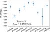 |
Fig. 1 The peak J absolute magnitude distribution for the calibrator SN Ia sample, based on the Cepheid distances of Riess et al. (2016). The data have been corrected for Milky Way extinction and K-corrections, but no further light curve shape or colour correction is applied. |
In the same way as for the calibrator sample, we derive peak apparent magnitudes mJ and uncertainties σfit for the Hubble-flow sample from the Gaussian process interpolation, applying Milky Way extinction and K-corrections as above. For the K-corrections, we warp the model SED to match the SN colour (using the mangle option in SNooPy; Burns et al. 2011). The difference between colour-matching and not colour-matching the SED is small (≲0.01 mag) for all SNe. For SNe that have Y and H band observations we use the Y, J, and H filters to match colours, otherwise we use J, H, and K filters. The former approach is more reliable, as pointed out by Boldt et al. (2014); nonetheless these differences are small for SNe in our sample (≲0.01 mag). For four objects (SN 2005eq, SN 2006lf, PTF10mwb, and PTF10ufj), the default Gaussian process covariance function parameters do not produce a satisfactory fit. For these objects, we reduce the scale and increase the amplitude of the covariance function (the parameters are specified in the fitting module code). Our final results are listed in Table 2.
We retrieved CMB-frame redshifts for the Hubble-flow host galaxies from NED2. These are largely consistent with values previously reported in the literature, except for NGC 2930, host of SN 2005M, which has a previously erroneous redshift now corrected in NED. Four of our Hubble-flow host galaxies are cluster members: for these we take the cosmological redshift as the cluster redshift reported in NED rather than the specific host galaxy redshift to avoid large peculiar velocities from the cluster velocity dispersion. These objects are noted in Table 2. Following the analysis of Riess et al. (2016), we also tabulate redshifts corrected for coherent flows derived from a model based on visible large scale structure (Carrick et al. 2015). Along with the reported redshift uncertainties σz, we adopt an additional peculiar velocity uncertainty of σpec = 150kms-1 (for all SNe except PTF10ufj the redshift uncertainty is sub-dominant compared to the peculiar velocity uncertainty).
The high precision of modern SN Ia H0 measurements (Riess et al. 2009, 2011, 2016) is due in part to selecting an “ideal” set of calibrator SN Ia, with low extinction and typical light curve shapes. The Hubble-flow SN Ia are a much more heterogeneous set than these ideal calibrators. Given that we are not applying colour or light curve shape corrections and treating the SN Ia as standard candles in their peak J magnitude, it is important to ensure that our Hubble-flow objects are on the whole similar to the calibrators. In Fig. 2, we plot the Hubble-flow Hubble diagram residuals and calibrator absolute magnitudes on the same scale, as a function of host-galaxy morphology and two parameters estimated from the optical light curves of these SN Ia: host galaxy reddening E(B−V) and light-curve decline rate Δm15(B) (Phillips 1993; Hamuy et al. 1996). These quantities are taken from the literature and tabulated in Table 3; we have not attempted to derive them in a uniform way. Rather, we are interested in comparing the Hubble-flow and calibrator SN Ia to suggest sample cuts. Beyond that, we do not use the optical photometry in any way in our results.
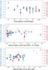 |
Fig. 2 A comparison of the calibrator and Hubble-flow samples in host-galaxy morphology, host-galaxy reddening, and optical light-curve decline rate. Blue circles show the Hubble-flow sample J-band Hubble-diagram residuals (left axis), while red squares show the calibrator absolute J magnitudes (right axis). The open circles indicate three fast-declining SN Ia that are excluded from our fiducial sample as outliers. These plots are used to define sample cuts only. Distances are based on the J-band photometry alone, with no corrections from these diagnostic parameters. |
Host-galaxy reddening, light-curve decline rate, and host-galaxy morphology for the calibrator and Hubble-flow SN Ia, compiled from the literature.
Figure 2 shows that the Hubble-flow SN Ia span a broader range of the displayed diagnostic parameters than the calibrators. This is to be expected. For example, the calibrator galaxies are chosen to host Cepheids, excluding early-type galaxies. Similarly the “ideal” calibrators have low host reddening and normal decline rates. Nonetheless, the visual impression from Fig. 2 is that the broader Hubble-flow sample does not show obvious trends with the parameters, except for the three fast-declining (Δm15(B) > 1.7) SN Ia, which are clear outliers (open circles). Indeed, Krisciunas et al. (2009), Kattner et al. (2012), and Dhawan et al. (2017b) have demonstrated that the NIR absolute magnitudes of fast-declining SN Ia diverge considerably from their more normal counterparts (similar to the behaviour in optical bands). We define a fiducial sample for analysis excluding these three SN Ia, and explore further sample cuts in Sect. 4.1.
The Hubble diagram of our fiducial sample, with 27 objects in the Hubble flow, is shown in Fig. 3. The standard deviation of the residuals is just σHflow = 0.106 mag in our simple standard-candle approach. Very few optical SN Ia samples have such a low scatter, even after light curve shape and colour correction. This scatter includes known components like the photometry and redshift measurement uncertainties and peculiar velocities. We convert the redshift/velocity uncertainties to magnitudes, with  (1)and adopt σpec = 150kms-1 as noted above. The individual Hubble-flow object uncertainty is then the quadrature sum of these terms and the Gaussian process fit peak magnitude uncertainty,
 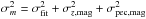 .
.
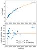 |
Fig. 3 Hubble diagram for our fiducial sample of 27 Hubble-flow SN Ia. |
As for the calibrators, though to a lesser extent, the Hubble-flow sample shows more scatter than can be explained by the formal uncertainties, here with χ2 = 62.8 for 26 degrees of freedom. Again, this points to the need for an additional intrinsic scatter component to explain the variance in the data.
Combining the calibrator sample and the Hubble-flow sample yields our estimate of H0, with  (2)for the luminosity distance dL measured in Mpc. Following Riess et al. (2016) we use a kinematic expression for the luminosity distance-redshift relation, with
 ![Mathematical equation: \begin{equation} d_{\rm L}(z) = \frac{cz}{H_0}\left[1+\frac{(1-q_0)z}{2} - \frac{(1 - q_0 - 3 q^2_0 + j_0)z^2}{6} + \mathcal{O}(z^3)\right] \label{eq:klumdist} \end{equation}](/articles/aa/full_html/2018/01/aa31501-17/aa31501-17-eq95.png) (3)and we fix q0 = −0.55 and j0 = 1. We have also explored the dynamic parametrisation of the luminosity distance in a flat, ΩM + ΩΛ = 1, Universe (see, e.g., Jha et al. 2007),
(3)and we fix q0 = −0.55 and j0 = 1. We have also explored the dynamic parametrisation of the luminosity distance in a flat, ΩM + ΩΛ = 1, Universe (see, e.g., Jha et al. 2007), ![Mathematical equation: \begin{equation} d_{\rm L}(z) = \frac{c(1+z)}{H_0}\int_0^z \left[\Omega_{\rm M}(1 + z')^3 + \Omega_\Lambda\right]^{-1/2} {\rm d}z'. \end{equation}](/articles/aa/full_html/2018/01/aa31501-17/aa31501-17-eq99.png) (4)Because our Hubble-flow sample is at quite low redshift, we find no significant differences in our results with either approach, nor when varying cosmological parameters within their observational limits.
(4)Because our Hubble-flow sample is at quite low redshift, we find no significant differences in our results with either approach, nor when varying cosmological parameters within their observational limits.
In estimating H0 from SN Ia it is traditional to rewrite Eqs. (2) and (3) as  (5)where MJ is constrained by the calibrator sample, and aJ is the “intercept of the ridge line” that can be determined separately from the Hubble-flow sample. Ignoring higher order terms, the intercept is given by
 ![Mathematical equation: \begin{equation} a_J = \log cz + \log \left[1+\frac{(1-q_0)z}{2} - \frac{(1 - q_0 - 3 q^2_0 + j_0)z^2}{6}\right] - 0.2 m_J. \label{eq:intercept} \end{equation}](/articles/aa/full_html/2018/01/aa31501-17/aa31501-17-eq102.png) (6)We vary the traditional analysis slightly to account for the necessary intrinsic scatter parameter, σint, that we interpret as supernova to supernova variance in the peak J luminosity. We introduce σint as a nuisance parameter that is to be constrained by the data and marginalized over. We assume that the intrinsic scatter is a property of the supernovae, independent of whether an object is in the calibrator sample or the Hubble-flow sample (and test this assumption in Sect. 4.2). In this case the full uncertainty for a given calibrator object i is
(6)We vary the traditional analysis slightly to account for the necessary intrinsic scatter parameter, σint, that we interpret as supernova to supernova variance in the peak J luminosity. We introduce σint as a nuisance parameter that is to be constrained by the data and marginalized over. We assume that the intrinsic scatter is a property of the supernovae, independent of whether an object is in the calibrator sample or the Hubble-flow sample (and test this assumption in Sect. 4.2). In this case the full uncertainty for a given calibrator object i is  (7)and the total uncertainty for a Hubble-flow object k is
  (8)Because the same intrinsic scatter affects the relative weights of both calibrator and Hubble-flow objects, we cannot solve for MJ and aJ independently. Instead we fit a joint Bayesian model to the combined data set, with MCMC sampling of the posterior distribution using the emcee package (Foreman-Mackey et al. 2013a,b). In principle we have four fit parameters: MJ, aJ, σint, and H0, but we can simplify this to just three using Eq. (5). We choose H0, MJ, and σint as our parameterisation, and simply calculate aJ for each MCMC sample given H0 and MJ. The results would be identical if we had fit for aJ and calculated H0. For convenience, rather than aJ, we tabulate −5aJ which can be expressed in units of magnitudes and interpreted in the same sense as the Hubble-flow peak magnitudes mJ. In our Bayesian analysis we take uninformative priors: uniform on H0> 0 and MJ, and scale-free on σint> 0, with p(σint) = 1 /σint. Our full analysis code, including notebooks that produce Figs. 1–4, is available online3.
4. Results
Our fiducial sample consists of the 9 calibrator SN Ia and 27 Hubble-flow SN Ia (i.e., excluding the three fast-declining outliers). We use the NED redshifts and uncertainties (Cols. 3 and 4 of Table 2) for the Hubble-flow objects. The results from 2 × 10⁵ posterior samples of our model are shown in Fig. 4 and tabulated in Table 4. We find a sample median  kms-1Mpc-1, where the uncertainty is statistical only, and is measured down (up) to the 16th (84th) percentile4. The 2.2% statistical uncertainty is impressive given the small sample size. The results show that the median calibrator peak magnitude (MJ = −18.524 ± 0.041) contributes approximately 2% uncertainty to H0 , whereas the Hubble flow sample contributes about 1% (−5aJ = −2.834 ± 0.023 mag), in line with the numbers of supernovae in each category.
We also see the intrinsic scatter parameter is estimated clearly to be non-zero:  . This has the effect of increasing the uncertainties in the other parameters, for instance, roughly doubling the uncertainty on the peak absolute magnitude MJ compared to the straight weighted mean calculated in Sect. 3. Though our analysis method was developed to allow the intrinsic scatter parameter to connect to both the calibrator and Hubble-flow samples, we further see in Fig. 4 that MJ and −5aJ do not have much correlation, reflecting the fact they are largely being constrained separately by the calibrators and Hubble-flow objects, respectively.
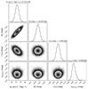 |
Fig. 4 Distribution and covariances of the model parameters for our fiducial sample. The uncertainties are statistical only, with the median value and 16th and 84th percentile differences listed. As discussed in the text, aJ is not a fit parameter; it is calculated from the other parameters for each sample. This plot uses the corner package by Foreman-Mackey (2017). |
Results with varying sample choices.
4.1. SN sample choices
To explore the sensitivity of our derived H0 , in Table 4 we present a number of different sample choices. First, we find that adopting the flow corrections to the CMB frame redshifts from Table 2 has only a small effect, raising H0 by 0.5% (0.4 kms-1Mpc-1), though also slightly increasing the Hubble-flow scatter from 0.106 mag to 0.115 mag. Because of the increased scatter, we do not adopt these flow corrections for our fiducial sample.
Similarly, restricting the Hubble-flow sample to low host reddening, low Milky Way extinction, or spiral galaxies only has little effect on the derived H0 or intrinsic scatter. Combining these three cuts does decrease the Hubble flow scatter slightly to 0.094 mag at the expense of eliminating nearly half of the Hubble flow sample; this combination yields H0 that is 1% higher than the fiducial sample.
Limiting the redshift range of the Hubble-flow sample similarly has little effect as shown in Table 4, 1.6% higher at most if the sample is reduced to just the 12 objects with 0.02 ≤ z ≤ 0.05. If we make an even more extreme cut, identifying both calibrator and Hubble flow objects that overlap in their diagnostics from Fig. 2, we retain only 7 calibrators and 8 Hubble-flow objects. Even so, the derived value of H0 in this “strictest overlap” sample shows no significant deviation than from the larger, fiducial sample.
On the other hand, if we include the three fast-declining “outlier” SN Ia, these fainter objects (Krisciunas et al. 2009; Dhawan et al. 2017b) pull the value of H0 down to 71.3 ± 2.1kms-1Mpc-1 (a 2.0% decrease), while increasing the Hubble flow scatter significantly, from 0.106 to 0.170 mag. As seen in Fig. 2, these fast-declining Hubble-flow objects clearly have no calibrator analogues and should be excluded.
4.2. Intrinsic scatter
The derived value of the intrinsic scatter for the fiducial sample, mag seems reasonable compared to optical SN Ia distances after standardization. Nevertheless, adopting a single intrinsic scatter may serve to obscure systematic uncertainties. In particular, we note that the dispersion of the residuals of the fiducial Hubble flow sample is 0.106 mag (which includes the measured photometric and redshift uncertainties as well as peculiar velocity uncertainties), substantially less than the scatter in the calibrators, 0.160 mag (including photometric and Cepheid distance uncertainties). We can test these for consistency by including two separate intrinsic scatter parameters, one for the calibrators and one for the Hubble flow. In that case, we find 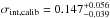 mag and
 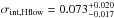 mag. These are only consistent at the ~2σ level. Marginalizing over both of these parameters, our fiducial value of H0 is not significantly changed, but has slightly higher uncertainty,
  kms-1Mpc-1, corresponding to 2.8% precision rather than 2.2%. This is mainly due to the higher intrinsic scatter in the calibrators, for which the peak absolute magnitude is now measured to lower precision: MJ = −18.524 ± 0.057 mag.
Separating the intrinsic scatter in this manner leads to some other complications. In principle the Hubble-flow intrinsic scatter parameter, which is independent of redshift, should be separable from the adopted peculiar velocity uncertainty (which for a fixed velocity uncertainty, corresponds to larger magnitude uncertainty at lower redshifts; Eq. (1)). However, because the redshift range of our Hubble-flow sample is small, in practice the Hubble-flow intrinsic scatter is largely degenerate with the adopted peculiar velocity uncertainty. Raising σpec to 250 kms-1, as used in Riess et al. (2016), completely accounts for all the Hubble flow scatter, and yields  mag, clearly inconsistent with the scatter in the calibrators. Conversely, if we unrealistically assume σpec = 0, the intrinsic scatter parameter increases to explain the observed scatter,
 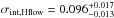 mag. Regardless of the exact choice, the marginalized result for H0 is largely unaffected, differing only by ±0.1 kms-1Mpc-1 relative to our fiducial choice of σpec = 150kms-1. Our choice is plausible (Radburn-Smith et al. 2004; Turnbull et al. 2012; Feindt et al. 2013) and previous studies have also used this value for the peculiar velocity uncertainty (Mandel et al. 2009, 2011; Barone-Nugent et al. 2012). Nevertheless, the higher scatter in the calibrator sample compared to the larger Hubble flow sample is a concern that should be noted; any systematic differences between the calibrators and the Hubble-flow objects could create a bias in H0 . Augmenting both of these samples in the future should clarify the situation.
4.3. Systematic uncertainties
In this study, we assume that SNe Ia are standard candles in the J-band; we do not correct for the light curve shape or host galaxy reddening. From Fig. 2 we see that these parameters are not significantly different for the calibrators and the Hubble flow objects. For example, the average difference (fiducial Hubble flow minus calibrators) in E(B−V)host is just 0.023 ± 0.043 mag. For AJ ≈ 0.8 E(B−V), this corresponds to a potential 1 ± 2% correction to H0 . Curiously, in the middle panel of Fig. 2, we do not see any evidence that objects with larger E(B−V)host are observed to be fainter (positive residuals). Given the data in Table 3 show a mild anti-correlation between E(B−V)host and Δm15(B), there could be a fortuitous cancellation between a colour correction and a light-curve shape dependence like that found by (Kattner et al. 2012). In Table 4 we note that restricting the samples to low E(B−V)host ≤ 0.3 mag does not change H0 significantly. Similarly, Fig. 2 shows that for the fiducial sample (excluding the fast-declining objects), there are no strong trends in residual with host galaxy morphology or optical light curve shape. Were we to regress these parameters and make corrections, our derived H0 would not significantly change. Based on this analysis, we adopt a ±1% systematic uncertainty from these potential sample differences.
Best fit J-band peak magnitudes for the two Hubble-flow SNe observed by both CSP and CfA.
One source of uncertainty that is systematically different between the calibrators and the Hubble-flow sample is K-corrections. There are not as many near infrared spectra of SNe Ia as in the optical, and ground-based observations are complicated by atmospheric absorption. Nevertheless, the median redshift of our Hubble-flow sample is only zmed = 0.018, where the K-correction uncertainties are ~0.015 mag (Boldt et al. 2014; Stanishev et al. 2015), corresponding to only a ~0.7% uncertainty in H0 .
Our Hubble-flow sample is drawn largely from two surveys: CSP (Contreras et al. 2010; Stritzinger et al. 2011) and CfA (Wood-Vasey et al. 2008; Friedman et al. 2015). Friedman et al. (2015) do an extensive comparison of CfA and CSP NIR photometry for 18 SNe Ia in common, and find a mean offset in J of just ⟨ΔmJ(CSP−CfA)⟩ = −0.004 ± 0.004 mag. Two of these objects, SN 2005el and SN 2008hv, have the requisite light-curve coverage to qualify for our Hubble-flow sample. Table 5 shows the excellent agreement in peak mJ for these objects when comparing the two surveys and justifies our combining the photometry for these two objects in our fiducial sample.
Despite these extensive cross-checks between the surveys, Table 4 shows the intercept of the ridge line (in the form of −5aJ) differs by 0.078 mag between the CSP and CfA Hubble-flow samples, translating into a ~3.7% difference in H0 . Unfortunately six of the nine calibrators have their J-band photometry from sources other than these surveys, so it is difficult to simply restrict our analysis to one system or the other. Table 4 presents results for the CSP Hubble-flow sample with the one calibrator with CSP photometry (SN 2007af) and similarly the CfA Hubble-flow sample with two CfA calibrators (SN 2011by and SN 2012cg), but these calibrator samples are too small to meaningfully estimate an intrinsic scatter and determine a secure value for H0 . The variety of photometric systems for the calibrator sample may help explain its higher scatter compared to the Hubble flow sample. Filter corrections (S-corrections; Stritzinger et al. 2002; Friedman et al. 2015) are expected to be modest in J-band at peak (the supernova NIR color is within the stellar locus), so zero-point differences may play the largest role. Here we adopt a ±3% systematic uncertainty on H0 from the average difference between the calibrators and Hubble-flow sample based on the different photometric systems. Our information is too limited here to better quantify this uncertainty, but this estimate makes it the largest component in the systematic error budget and a ripe target for future improvement.
Combining these effects our near infrared “supernova” standard candle systematic uncertainty amounts to 3.2%. Our estimate of H0 also relies on the Cepheid distances of Riess et al. (2016) and thus we adopt their systematic uncertainties (see their Table 7) for the lower rungs of the distance ladder including the primary anchor distance, the mean Leavitt Law in the anchors, the mean Leavitt Law in the calibrator host galaxies (corrected for the fact we only use 9 calibrators rather than 19 as in Riess et al. 2016), Cepheid reddening and metallicity corrections, and other Leavitt Law uncertainties. This gives a “Cepheid+anchor” systematic uncertainty of 1.8%.
To check this we have analysed our sample using the alternate Cepheid distances from Cardona et al. (2017), who introduce hyper-parameters to account for outliers and other potential systematic uncertainties in the data set. For our calibrators, the differences based on this reanalysis are minor, mainly somewhat increased uncertainties in a few of the Cepheid distances. The biggest change is for NGC 4424 (host of SN 2012cg), for which Cardona et al. (2017) find μCeph = 30.82 ± 0.19 mag compared to 31.08 ± 0.29 mag from Riess et al. (2016). In fact this reduces the scatter for the 9 calibrators from 0.160 mag to 0.133 mag, as shown in Table 4, and increases H0 by 1.4% compared to our fiducial analysis, well within the 1.8% Cepheid+anchor systematic uncertainty.
Summing our supernova (3.2%) plus Cepheid+anchor (1.8%) systematic uncertainties in quadrature yields our total systematic uncertainty of 3.7%, and gives our final estimate of H0 = 72.8 ± 1.6 (statistical) ±2.7 (systematic) kms-1Mpc-1. Our result is completely consistent with Riess et al. (2016). Because the Cepheid and anchor data we adopt is from that analysis, those uncertainties are in common and our near infrared cross-check of their result is actually more precise. Our result can be written H0 = 72.8 ± 1.6 (statistical) ±2.3 (separate systematics) ±1.3 (in common systematics) kms-1Mpc-1. Leaving out the in-common systematics we can compare our result 72.8 ± 2.8kms-1Mpc-1 with the Riess et al. (2016) result (also leaving out systematics in common, which dominate their error budget), 73.2 ± 0.8kms-1Mpc-1 and find excellent agreement5.
5. Discussion and conclusion
Our main conclusion is that replacing optical light curve standardized distances of SNe Ia with J-band standard candle distances gives a wholly consistent (at lower precision) distance ladder and measurement of the H0. This suggests that supernova systematic uncertainties that could be expected to vary with wavelength (e.g., dust extinction or colour correction) are not likely to play a dominant role in “explaining” the tension between the local measurement of H0 and its inference from CMB data in a standard cosmological model. Studies have sought to determine whether or not SN Ia luminosity variations relate to local environments in nearby samples (z ≲ 0.1; Rigault et al. 2013, 2015; Kelly et al. 2015; Jones et al. 2015; Roman et al. 2017). To play a dominant role, such environmental factors must affect both the optical and J-band light curves in common.
Our final result has lower precision than the Riess et al. (2016), with total (statistical+systematic) uncertainty of 4.3%: 72.8 ± 3.1kms-1Mpc-1. We can still compare this with the reverse distance ladder estimate from the 2016 Planck intermediate results: 66.93 ± 0.62kms-1Mpc-1 (Planck Collaboration Int. XLVI 2016), and find a 1.8σ “tension”. The significance of this would be increased had we posited a priori that we were only checking for a local value that was higher than the CMB value (i.e., a one-tailed test).
A number of aspects of our analysis can be improved, both in terms of statistical and systematic uncertainty. Our calibrator sample size is less than half that of Riess et al. (2016), and our Hubble-flow sample nearly an order of magnitude smaller (and at typically lower redshift, more susceptible to peculiar velocities). Our statistical uncertainty would be improved by more objects in both sets: more Cepheid-calibrated SN Ia and importantly, more well-sampled near infrared light curves of nearby and Hubble-flow SN Ia. Our limited sample is due in part to our stringent requirement for NIR data before J-band maximum light. This peak typically occurs a few days before B-band maximum light, and has been difficult to measure. New surveys that discover nearby SN Ia earlier, combined with rapid NIR follow-up will certainly help.
Of course, we do not need to use only the J-band peak magnitude. For example, H-band is even less sensitive to dust and may provide an even better standard candle (Kasen 2006; Wood-Vasey et al. 2008; Mandel et al. 2009, 2011; Weyant et al. 2014). However, the H-band “peak” is much broader in time and not as well-defined as in J, making it difficult to measure in our approach. Fitting template NIR light-curves (e.g. Wood-Vasey et al. 2008; Folatelli et al. 2010; Burns et al. 2011; Kattner et al. 2012) would allow for additional filters and sparser light-curve coverage. It will be important to test whether data from later epochs has increased scatter relative to the J-band peak; for instance, in the redder optical bands, the second maximum does show more variation among SNe (Hamuy et al. 1996; Jha et al. 2007; Dhawan et al. 2015). In addition, here we measure the peak J magnitude at the time of J maximum; previous studies have often measured the “peak” magnitude at the time of B maximum. These times of maxima can show systematic variations (Krisciunas et al. 2009; Kattner et al. 2012) that could lead to a different magnitude scatter between the two approaches.
Systematic uncertainties can also be mitigated. We have ascribed our dominant systematic uncertainty to photometric calibration of the J-band data, as evidenced by the difference in Hubble-flow intercepts from CSP and CfA, and perhaps the increased scatter in the calibrator sample (which has more heterogeneous photometric sources). Further in-depth analysis of the photometry (already discussed extensively in Friedman et al. 2015) could in principle significantly reduce this uncertainty. Augmented NIR spectroscopic templates could better quantify K- and S-correction uncertainties. Finally, we performed our analysis unblinded, raising the possibility of confirmation bias in our results. Future analyses can be designed with a blinded methodology, as recently applied to this problem by Zhang et al. (2017).
Perhaps the most remarkable of our results is how well a purely standard candle approach works, with intrinsic (unmodeled) scatter comparable to optical light curves after correction. Measuring and applying corrections to the NIR light curves (based on light-curve shape, colour, host galaxy properties, local environments, etc.) should only serve to increase the precision. NIR observations of SNe Ia may thus play a key role in a distance ladder that makes the best future measurements of the local value of H0 , an extremely valuable cosmological constraint.
Riess et al. (2016) also explore a limit of z > 0.0233 for the Hubble flow; only 99 of the 213 SNe Ia would pass this redshift cut.
As seen in Fig. 4, the marginal distributions are largely symmetric, so using the medians or means give similar results.
Because Riess et al. (2016) used flow corrections for the Hubble flow sample, perhaps the best comparison is our flow-corrected redshifts value (Table 4), which coincidentally matches their value.
Acknowledgments
We are grateful to Adam Riess and Dan Scolnic for helpful comments. We thank Michael Foley for supplying the flow model velocity corrections. We appreciate useful discussions with Arturo Avelino, Anupam Bhardwaj, Chris Burns, Regis Cartier, Andrew Friedman, Kate Maguire, Kaisey Mandel, and Michael Wood-Vasey. We thank the anonymous referee for helpful suggestions. B.L. acknowledges support for this work by the Deutsche Forschungsgemeinschaft through TRR33, The Dark Universe. This research was supported by the Munich Institute for Astro- and Particle Physics (MIAPP) of the DFG cluster of excellence “Origin and Structure of the Universe”. S.W.J. acknowledges support from US Department of Energy grant DE-SC0011636 and valuable discussion and collaboration opportunity during the MIAPP program “The Physics of Supernovae”.
References
- Alam, S., Ata, M., Bailey, S., et al. 2017, MNRAS, 470, 2617 [NASA ADS] [CrossRef] [Google Scholar]
- Barone-Nugent, R. L., Lidman, C., Wyithe, J. S. B., et al. 2012, MNRAS, 425, 1007 [NASA ADS] [CrossRef] [Google Scholar]
- Barone-Nugent, R. L., Lidman, C., Wyithe, J. S. B., et al. 2013, MNRAS, 432, L90 [NASA ADS] [CrossRef] [Google Scholar]
- Bennett, C. L., Larson, D., Weiland, J. L., et al. 2013, ApJS, 208, 20 [Google Scholar]
- Betoule, M., Kessler, R., Guy, J., et al. 2014, A&A, 568, A22 [NASA ADS] [CrossRef] [EDP Sciences] [Google Scholar]
- Boldt, L. N., Stritzinger, M. D., Burns, C., et al. 2014, PASP, 126, 324 [NASA ADS] [CrossRef] [Google Scholar]
- Bonvin, V., Courbin, F., Suyu, S. H., et al. 2017, MNRAS, 465, 4914 [NASA ADS] [CrossRef] [Google Scholar]
- Burns, C. R., Stritzinger, M., Phillips, M. M., et al. 2011, AJ, 141, 19 [NASA ADS] [CrossRef] [Google Scholar]
- Cardona, W., Kunz, M., & Pettorino, V. 2017, JCAP, 3, 056 [NASA ADS] [CrossRef] [Google Scholar]
- Carrick, J., Turnbull, S. J., Lavaux, G., & Hudson, M. J. 2015, MNRAS, 450, 317 [NASA ADS] [CrossRef] [Google Scholar]
- Cartier, R., Hamuy, M., Pignata, G., et al. 2014, ApJ, 789, 89 [NASA ADS] [CrossRef] [Google Scholar]
- Cartier, R., Sullivan, M., Firth, R. E., et al. 2017, MNRAS, 464, 4476 [NASA ADS] [CrossRef] [Google Scholar]
- Contreras, C., Hamuy, M., Phillips, M. M., et al. 2010, AJ, 139, 519 [NASA ADS] [CrossRef] [Google Scholar]
- Dhawan, S., Leibundgut, B., Spyromilio, J., & Maguire, K. 2015, MNRAS, 448, 1345 [NASA ADS] [CrossRef] [Google Scholar]
- Dhawan, S., Goobar, A., Mörtsell, E., Amanullah, R., & Feindt, U. 2017a, JCAP, 07, 040 [NASA ADS] [CrossRef] [Google Scholar]
- Dhawan, S., Leibundgut, B., Spyromilio, J., & Blondin, S. 2017b, A&A, 602, A118 [NASA ADS] [CrossRef] [EDP Sciences] [Google Scholar]
- Di Valentino, E., Melchiorri, A., & Mena, O. 2017, Phys. Rev. D, 96, 043503 [NASA ADS] [CrossRef] [Google Scholar]
- Feeney, S. M., Mortlock, D. J., & Dalmasso, N. 2017, MNRAS, submitted [arXiv:1707.00007] [Google Scholar]
- Feindt, U., Kerschhaggl, M., Kowalski, M., et al. 2013, A&A, 560, A90 [NASA ADS] [CrossRef] [EDP Sciences] [Google Scholar]
- Folatelli, G., Phillips, M. M., Burns, C. R., et al. 2010, AJ, 139, 120 [NASA ADS] [CrossRef] [Google Scholar]
- Follin, B., & Knox, L. 2017, ArXiv e-prints [arXiv:1707.01175] [Google Scholar]
- Foreman-Mackey, D. 2017, Astrophysics Source Code Library [record ascl:1702.002] [Google Scholar]
- Foreman-Mackey, D., Conley, A., Meierjurgen Farr, W., et al. 2013a, Astrophysics Source Code Library [record ascl:1303.002] [Google Scholar]
- Foreman-Mackey, D., Hogg, D. W., Lang, D., & Goodman, J. 2013b, PASP, 125, 306 [CrossRef] [Google Scholar]
- Freedman, W. L., Madore, B. F., Scowcroft, V., et al. 2012, ApJ, 758, 24 [NASA ADS] [CrossRef] [Google Scholar]
- Friedman, A. S., Wood-Vasey, W. M., Marion, G. H., et al. 2015, ApJS, 220, 9 [NASA ADS] [CrossRef] [Google Scholar]
- Guy, J., Astier, P., Baumont, S., et al. 2007, A&A, 466, 11 [NASA ADS] [CrossRef] [EDP Sciences] [Google Scholar]
- Hamuy, M., Phillips, M. M., Suntzeff, N. B., et al. 1996, AJ, 112, 2438 [NASA ADS] [CrossRef] [Google Scholar]
- Hicken, M., Challis, P., Jha, S., et al. 2009, ApJ, 700, 331 [NASA ADS] [CrossRef] [Google Scholar]
- Hicken, M., Challis, P., Kirshner, R. P., et al. 2012, ApJS, 200, 12 [NASA ADS] [CrossRef] [Google Scholar]
- Hinshaw, G., Larson, D., Komatsu, E., et al. 2013, ApJS, 208, 19 [NASA ADS] [CrossRef] [Google Scholar]
- Hsiao, E. Y., Conley, A., Howell, D. A., et al. 2007, ApJ, 663, 1187 [NASA ADS] [CrossRef] [Google Scholar]
- Jha, S., Riess, A. G., & Kirshner, R. P. 2007, ApJ, 659, 122 [NASA ADS] [CrossRef] [Google Scholar]
- Jones, D. O., Riess, A. G., & Scolnic, D. M. 2015, ApJ, 812, 31 [NASA ADS] [CrossRef] [Google Scholar]
- Kasen, D. 2006, ApJ, 649, 939 [NASA ADS] [CrossRef] [Google Scholar]
- Kattner, S., Leonard, D. C., Burns, C. R., et al. 2012, PASP, 124, 114 [NASA ADS] [CrossRef] [Google Scholar]
- Kelly, P. L., Filippenko, A. V., Burke, D. L., et al. 2015, Science, 347, 1459 [NASA ADS] [CrossRef] [Google Scholar]
- Krisciunas, K., Phillips, M. M., & Suntzeff, N. B. 2004, ApJ, 602, L81 [NASA ADS] [CrossRef] [Google Scholar]
- Krisciunas, K., Marion, G. H., Suntzeff, N. B., et al. 2009, AJ, 138, 1584 [NASA ADS] [CrossRef] [Google Scholar]
- Leavitt, H. S., & Pickering, E. C. 1912, Harvard College Observatory Circular, 173, 1 [Google Scholar]
- Macri, L. M., Ngeow, C.-C., Kanbur, S. M., Mahzooni, S., & Smitka, M. T. 2015, AJ, 149, 117 [NASA ADS] [CrossRef] [Google Scholar]
- Maguire, K., Sullivan, M., Ellis, R. S., et al. 2012, MNRAS, 426, 2359 [NASA ADS] [CrossRef] [Google Scholar]
- Mandel, K. S., Wood-Vasey, W. M., Friedman, A. S., & Kirshner, R. P. 2009, ApJ, 704, 629 [NASA ADS] [CrossRef] [Google Scholar]
- Mandel, K. S., Narayan, G., & Kirshner, R. P. 2011, ApJ, 731, 120 [NASA ADS] [CrossRef] [Google Scholar]
- Marion, G. H., Brown, P. J., Vinkó, J., et al. 2016, ApJ, 820, 92 [NASA ADS] [CrossRef] [Google Scholar]
- Matheson, T., Joyce, R. R., Allen, L. E., et al. 2012, ApJ, 754, 19 [NASA ADS] [CrossRef] [Google Scholar]
- Meikle, W. P. S. 2000, MNRAS, 314, 782 [NASA ADS] [CrossRef] [Google Scholar]
- Phillips, M. M. 1993, ApJ, 413, L105 [NASA ADS] [CrossRef] [Google Scholar]
- Planck Collaboration XIII. 2016, A&A, 594, A13 [NASA ADS] [CrossRef] [EDP Sciences] [Google Scholar]
- Planck Collaboration Int. XLVI. 2016, A&A, 596, A107 [NASA ADS] [CrossRef] [EDP Sciences] [Google Scholar]
- Radburn-Smith, D. J., Lucey, J. R., & Hudson, M. J. 2004, MNRAS, 355, 1378 [Google Scholar]
- Renk, J., Zumalacárregui, M., Montanari, F., & Barreira, A. 2017, JCAP, 10, 020 [NASA ADS] [CrossRef] [Google Scholar]
- Riess, A. G., Macri, L., Casertano, S., et al. 2009, ApJ, 699, 539 [NASA ADS] [CrossRef] [Google Scholar]
- Riess, A. G., Macri, L., Casertano, S., et al. 2011, ApJ, 730, 119 [NASA ADS] [CrossRef] [Google Scholar]
- Riess, A. G., Macri, L. M., Hoffmann, S. L., et al. 2016, ApJ, 826, 56 [NASA ADS] [CrossRef] [Google Scholar]
- Rigault, M., Copin, Y., Aldering, G., et al. 2013, A&A, 560, A66 [NASA ADS] [CrossRef] [EDP Sciences] [Google Scholar]
- Rigault, M., Aldering, G., Kowalski, M., et al. 2015, ApJ, 802, 20 [NASA ADS] [CrossRef] [Google Scholar]
- Roman, M., Hardin, D., Betoule, M., et al. 2017, ArXiv e-prints [arXiv:1706.07697] [Google Scholar]
- Sasankan, N., Gangopadhyay, M. R., Mathews, G. J., & Kusakabe, M. 2017, Phys. Rev. D, 95, 083516 [NASA ADS] [CrossRef] [Google Scholar]
- Schlafly, E. F., & Finkbeiner, D. P. 2011, ApJ, 737, 103 [NASA ADS] [CrossRef] [Google Scholar]
- Scolnic, D., Casertano, S., Riess, A., et al. 2015, ApJ, 815, 117 [NASA ADS] [CrossRef] [Google Scholar]
- Stanishev, V., Goobar, A., Benetti, S., et al. 2007, A&A, 469, 645 [NASA ADS] [CrossRef] [EDP Sciences] [Google Scholar]
- Stanishev, V., Goobar, A., Amanullah, R., et al. 2015, unpublished [arXiv:1505.07707] [Google Scholar]
- Stritzinger, M., Hamuy, M., Suntzeff, N. B., et al. 2002, AJ, 124, 2100 [NASA ADS] [CrossRef] [Google Scholar]
- Stritzinger, M. D., Phillips, M. M., Boldt, L. N., et al. 2011, AJ, 142, 156 [NASA ADS] [CrossRef] [Google Scholar]
- Suyu, S. H., Auger, M. W., Hilbert, S., et al. 2013, ApJ, 766, 70 [NASA ADS] [CrossRef] [Google Scholar]
- Turnbull, S. J., Hudson, M. J., Feldman, H. A., et al. 2012, MNRAS, 420, 447 [NASA ADS] [CrossRef] [Google Scholar]
- Verde, L., Bellini, E., Pigozzo, C., Heavens, A. F., & Jimenez, R. 2017, J. Cosmol. Astropart. Phys, 4, 023 [Google Scholar]
- Wang, X., Li, W., Filippenko, A. V., et al. 2009, ApJ, 697, 380 [NASA ADS] [CrossRef] [Google Scholar]
- Weyant, A., Wood-Vasey, W. M., Allen, L., et al. 2014, ApJ, 784, 105 [NASA ADS] [CrossRef] [Google Scholar]
- Weyant, A., Wood-Vasey, W. M., Joyce, R., et al. 2017, ApJS, submitted [arXiv:1703.02402] [Google Scholar]
- Wielgorski, P., Pietrzynski, G., Gieren, W., et al. 2017, ApJ, 842, 116 [NASA ADS] [CrossRef] [Google Scholar]
- Wood-Vasey, W. M., Friedman, A. S., Bloom, J. S., et al. 2008, ApJ, 689, 377 [NASA ADS] [CrossRef] [Google Scholar]
- Zhang, B. R., Childress, M. J., Davis, T. M., et al. 2017, MNRAS, 471, 2254 [NASA ADS] [CrossRef] [Google Scholar]
Appendix A: Gaussian process light curve fitting
In Sect. 3, we described the light curve fitting methodology for the SNe in our sample. In Fig. A.1 we plot the light curves of the 9 SNe in our calibration sample along with the Gaussian process fits to derive the peak magnitude. The same is plotted for the Hubble-flow sample in Fig. A.2.
 |
Fig. A.1 Gaussian Process Fits for SNe in the calibration sample. The errorbars are smaller than the point sizes in most cases. On the x-axis, the days from J-band maximum are in the observer frame. |
All Tables
The calibrator sample of Cepheid-calibrated SN Ia, with tabulated absolute magnitudes MJ and uncertainties σM.
CMB frame redshifts, with and without corrections for local flows, peak J-band magnitudes and uncertainties for SNe in the Hubble flow.
Host-galaxy reddening, light-curve decline rate, and host-galaxy morphology for the calibrator and Hubble-flow SN Ia, compiled from the literature.
Best fit J-band peak magnitudes for the two Hubble-flow SNe observed by both CSP and CfA.
All Figures
|
Fig. 1 The peak J absolute magnitude distribution for the calibrator SN Ia sample, based on the Cepheid distances of Riess et al. (2016). The data have been corrected for Milky Way extinction and K-corrections, but no further light curve shape or colour correction is applied. |
| In the text | |
|
Fig. 2 A comparison of the calibrator and Hubble-flow samples in host-galaxy morphology, host-galaxy reddening, and optical light-curve decline rate. Blue circles show the Hubble-flow sample J-band Hubble-diagram residuals (left axis), while red squares show the calibrator absolute J magnitudes (right axis). The open circles indicate three fast-declining SN Ia that are excluded from our fiducial sample as outliers. These plots are used to define sample cuts only. Distances are based on the J-band photometry alone, with no corrections from these diagnostic parameters. |
| In the text | |
|
Fig. 3 Hubble diagram for our fiducial sample of 27 Hubble-flow SN Ia. |
| In the text | |
|
Fig. 4 Distribution and covariances of the model parameters for our fiducial sample. The uncertainties are statistical only, with the median value and 16th and 84th percentile differences listed. As discussed in the text, aJ is not a fit parameter; it is calculated from the other parameters for each sample. This plot uses the corner package by Foreman-Mackey (2017). |
| In the text | |
|
Fig. A.1 Gaussian Process Fits for SNe in the calibration sample. The errorbars are smaller than the point sizes in most cases. On the x-axis, the days from J-band maximum are in the observer frame. |
| In the text | |
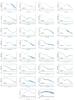 |
Fig. A.2 Same as Fig. A.1, but for the Hubble flow sample. |
| In the text | |
Current usage metrics show cumulative count of Article Views (full-text article views including HTML views, PDF and ePub downloads, according to the available data) and Abstracts Views on Vision4Press platform.
Data correspond to usage on the plateform after 2015. The current usage metrics is available 48-96 hours after online publication and is updated daily on week days.
Initial download of the metrics may take a while.