| Issue |
A&A
Volume 609, January 2018
|
|
|---|---|---|
| Article Number | A56 | |
| Number of page(s) | 6 | |
| Section | The Sun | |
| DOI | https://doi.org/10.1051/0004-6361/201731481 | |
| Published online | 05 January 2018 | |
Observing and modeling the poloidal and toroidal fields of the solar dynamo
Max-Planck-Institut für Sonnensystemforschung, 37077 Göttingen, Germany
e-mail: This email address is being protected from spambots. You need JavaScript enabled to view it.
Received: 30 June 2017
Accepted: 19 October 2017
Abstract
Context. The solar dynamo consists of a process that converts poloidal magnetic field to toroidal magnetic field followed by a process that creates new poloidal field from the toroidal field.
Aims. Our aim is to observe the poloidal and toroidal fields relevant to the global solar dynamo and to see if their evolution is captured by a Babcock-Leighton dynamo.
Methods. We used synoptic maps of the surface radial field from the KPNSO/VT and SOLIS observatories, to construct the poloidal field as a function of time and latitude; we also used full disk images from Wilcox Solar Observatory and SOHO/MDI to infer the longitudinally averaged surface azimuthal field. We show that the latter is consistent with an estimate of the longitudinally averaged surface azimuthal field due to flux emergence and therefore is closely related to the subsurface toroidal field.
Results. We present maps of the poloidal and toroidal magnetic fields of the global solar dynamo. The longitude-averaged azimuthal field observed at the surface results from flux emergence. At high latitudes this component follows the radial component of the polar fields with a short time lag of between 1−3 years. The lag increases at lower latitudes. The observed evolution of the poloidal and toroidal magnetic fields is described by the (updated) Babcock-Leighton dynamo model.
Key words: Sun: magnetic fields
© ESO, 2018
1. Introduction
The basic periodicity of the global dynamo of the Sun is about 22 years (Hale et al. 1919), consisting of two approximately 11 year activity cycles (Schwabe 1849). Typically, the first sunspots of an activity cycle appear before solar minimum, which is the traditional start time of a cycle, at latitudes of about ± 35°. The latitude at which they subsequently appear decreases as the cycle progresses until they reach about ± 8° at the end of the activity cycle (Carrington 1858; Spörer 1879). The appearance of sunspots marks the emergence of magnetic flux in the range of 5 × 10²¹ Mx to 3 × 10²² Mx through the solar surface (Schrijver & Zwaan 2000). The flux emerging in active regions (with fluxes from 1 × 10²⁰ to 3 × 10²² Mx) mostly obeys Hale’s law; this indicates that this flux comes from the subsurface toroidal field, which switches orientation from one cycle to the next.
Ephemeral regions have fluxes in the range of 3 × 10¹⁸ to 1 × 10²⁰ Mx. These regions have a statistical tendency to obey Hale’s law and begin emerging before the first sunspots of a cycle at higher latitudes (Martin & Harvey 1979; Harvey 1992). The earlier high-latitude emergences form part of the extended activity cycle (Wilson et al. 1988), which groups the activity at different latitudes associated with one cycle. The extended activity cycle is revealed in several different ways: coronal bright points and green-line emission (Altrock 1988; McIntosh et al. 2014), chromospheric plage (Harvey 1992), the emergence of bipoles preferentially obeying Hale’s law (Martin & Harvey 1979), the longitudinally averaged azimuthal inclination of photospheric magnetic flux (Howard 1974; Shrauner & Scherrer 1994; Lo et al. 2010), and the longitudinally averaged photospheric radial (Hathaway 2015) and azimuthal field (Duvall et al. 1979; Ulrich & Boyden 2005; Lo et al. 2010).
2. Observations of the radial and azimuthal fields
We determined the longitudinally averaged surface azimuthal field using the technique described in Duvall (1978) and Duvall et al. (1979) applied to WSO and SOHO/MDI observations. In brief, the technique first creates a very-deep line-of-sight magnetogram consisting of a yearly average of the line-of-sight magnetic field on the solar disk (for the SOHO/MDI data, each day is remapped first to account for B-angle variations). This average magnetogram is split into a component that is symmetric with respect to the solar meridian and a component that is anti-symmetric. Assuming that the position of the Earth does not affect the location of flux emergence, the anti-symmetric component at any latitude is proportional to the yearly and longitudinally averaged azimuthal field, shown in Fig. 1. Some differences between the results from the WSO and SOHO/MDI observations are expected because the two instruments have different spatial resolutions; for example, the WSO magnetograms do not resolve pores and spots.
During the years near solar maximum (2000 to 2003), the inferred surface azimuthally averaged azimuthal field in the active latitudes is between 1 G and 2 G. Around this time the inferred surface azimuthally averaged azimuthal field at high latitudes reverses and then grows to about 0.1 G, i.e., the overall level from 2007 to 2009 when the solar activity was low. The high-latitude azimuthal field after 2003 has the opposite sign in each hemisphere to the field in the low latitudes during maximum.
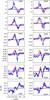 |
Fig. 1 Surface longitudinally averaged azimuthal field determined from MDI (blue) and Wilcox Solar Observatory (red). The pink and light blue shadings show the formal error bars of the fittings. |
The observable that corresponds to the relevant poloidal field of the global dynamo is the longitudinally averaged radial field at the solar surface (Cameron & Schüssler 2015), for which we have four activity cycles of observations, presented in the form of a time-latitude magnetic butterfly map (Hathaway 2015).
3. Observed surface toroidal flux as the result of flux emergence
While the observations are of the surface field, the relevant toroidal field for the solar dynamo is the subsurface longitudinally averaged azimuthal field, which we can only detect when it emerges through the surface. Emergences occur in the form of active regions at low latitudes during solar maximum and in the form of ephemeral regions over the entire Sun and throughout the cycle (Martin & Harvey 1979; Harvey 1992). Both active regions and ephemeral regions have a statistical tendency to follow Hale’s law; i.e., these regions are preferentially aligned in the east-west direction with the orientation corresponding to a particular activity cycle in each hemisphere. This means that more flux emerges with an east-west alignment corresponding to Hale’s law than disobeying Hale’s law. The difference between these two fluxes is a proxy for the underlying (axisymmetric) toroidal field. The preferential east-west alignment of the emerging flux in ephemeral regions shows up in the longitudinally averaged azimuthal field at the solar surface, which is directly observable as discussed in the previous section.
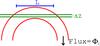 |
Fig. 2 Simplified geometry of a flux emergence event. The tube (shown in red) has flux Φi. The spatial extent of the emergence, the separation of the footpoints, is L. During emergence, the tube crosses the photospheric layer Δz (shown in green) where the polarimetric magnetograph signal is formed. |
To quantitatively estimate the average surface azimuthal field due to flux emergence, we use the simplified geometry shown in Fig. 2.
We are interested in the average over some area of the solar surface A and time T. Consider a single flux emergence event: a flux loop with azimuthal flux Φi that emerges over a length Li with tilt angle γi with respect to the azimuthal (EW) direction. The flux traverses the Zeeman-sensitive layer in the photosphere with an average radial speed, vr,i; the observable azimuthal field, Bφ,i(λ,φ,t), is only non-zero across the emerging region and during the emergence time, te, during which the full amount of the flux, Φi, traverses the Zeeman sensitive layer of the photosphere. Integrating over area A and time T we therefore have 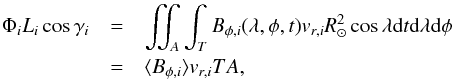 (1)where ⟨ Bφ,i ⟩ is the contribution of the emergence event to the average azimuthal field. The total average azimuthal field, ⟨ Bφ,i ⟩ is then given by the sum over all the emergence events across A and during time T, hence
 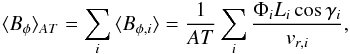 (2)where ⟨ ... ⟩ AT indicates the average over area A and time interval T.
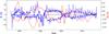 |
Fig. 3 High-latitude (λ> 50°) surface longitudinally averaged azithmuthal field from WS0 (red) and polar (λ> 80°) surface longitudinally averaged radial field from KPNSO/VT (blue). The northern (southern) polar data are shown with the solid (dashed) curves. |
In the case of ephemeral regions emerging in the quiet Sun, we use the results from Hagenaar (2001): the total amount of unsigned radial flux emerging in the form of ephemeral regions over the entire solar surface is about 5 × 10²³ Mx/day (1.8 × 1026 Mx/year), their spatial extent, L, is about 9 Mm, and about 60% of the ephemeral regions obey Hale’s law. This means 40 percent disobey Hale’s law compared to the 60% that obey Hale’s law. The resulting net flux preferentially obeying Hale’s law is hence 20% of the total emerging in the form of ephemeral regions, and the E-W aligned component of this is 63% of this total, assuming the regions obeying Hale’s law emerge with tilts with respect to the equator uniformly distributed in the range −90° to +90°. The rise velocity, vr, is on the order of about 1 km s-1 (e.g., Guglielmino et al. 2012), resulting in ⟨ Bφ ⟩ = 0.11 G (from Eq. (1)), where we have taken the average over T = 1 year and area A, which is the entire solar surface.
Considering the contribution from active regions emerging during maxima, we restrict the area A to the latitudinal extent of both butterfly wings (each of which has a latitudinal extent of about 16°; Cameron & Schüssler 2016), and again consider a yearly averaging. The rate at which flux emerges in the form of active regions was 2.3 × 1024 Mx/year during maximum of cycle 21 (Schrijver & Harvey 1994). The rise velocity, vr, of the toroidal flux through the photosphere in active regions can be estimated from the work of Centeno (2012). In that paper a range of radial velocities advecting the horizontal magnetic field across the photosphere in an emerging active region are reported. These include both radially outward and inward motions. We adopt vr = 100 m s-1 as the characteristic rise velocity, L = 40 Mm for a typical active region size, cosγ = 1 since there is less scatter in the tilt angle of large active regions than for ephemeral regions and T = 1 yr. Applying Eq. (1) results in a longitudinally averaged azimuthal field value of 1.7 G over the activity belts.
We therefore, find that the observed azimuthal field is quantitatively consistent with what we expect from flux emergence. In the quiet Sun, where flux emergence in the form of ephemeral regions dominates (e.g., most of the Sun during 2008), the observed average azimuthal field is on the order of 0.1 G (see Fig. 1), which is comparable to the estimate for the azimuthal field due to ephemeral regions. In the active Sun, where emergence in the form of active regions dominates, the observed field is on the order of 1 G, which is consistent with the expected value from flux emergence in the form of active regions.
Since flux emergence necessarily depends on the underlying toroidal field, the axisymmetric component of the azimuthal field determined at the surface in Fig. 1 represents a proxy of the subsurface toroidal field distribution of the global solar dynamo.
At high latitudes, the axisymmetric component of the azimuthal field follows the axisymmetric component of the radial component of the polar fields with a slight lag (1−3 yr), as can be seen in Fig. 3. The toroidal field at lower latitudes then follow at increasing time lags. This is very highly suggestive of a Babcock-Leighton flux transport dynamo where the field threading the poles is wound up by differential rotation and the resulting toroidal flux is advected equatorward. The advection of toroidal field away from the pole means that the toroidal field near the pole follows the polar fields with only a short delay, whereas at low latitudes the toroidal field of the new cycle must first replace the toroidal field that has already been transported equatorward owing to advection from higher latitudes.
4. Consistency with the Babcock-Leighton dynamo
A useful way of presenting the time and latitude dependence of the azimuthally averaged observed radial and azimuthal magnetic fields is in the form of magnetic butterfly diagrams, as shown in Fig. 4.
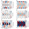 |
Fig. 4 Time-latitude diagrams of the observed (left) and simulated (right) magnetic fields. Panel a: observed surface longitudinally averaged radial field based on KPNSO/VT and SOLIS data. Panel b: observed surface longitudinally averaged toroidal magnetic field based on WSO observations, and panel c is the same as panel b except saturated to bring out the weaker high-latitude fields. Panel d: surface radial field from the updated Babcock-Leighton model (Cameron & Schüssler 2017), panel e: subsurface toroidal flux density from the Babcock-Leighton model, and panel f shows a saturated version of panel e. The black lines in all the panels show the zero contours from the model. |
Given that the observational data cover four cycles, we may now ask whether the observed evolution is captured by a Babcock-Leighton type dynamo. For this purpose we use the updated formulation of the model as presented in Cameron & Schüssler (2017). The model consists of two 1D evolution equations. The first describes the surface evolution of the poloidal field, 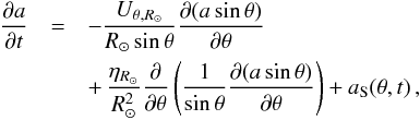 (3)where
 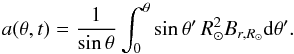 (4)The value Uθ,R⊙ is the surface meridional flow, ηR⊙ is the turbulent diffusion coefficient for the dispersion of radial field at the surface in the latitudinal direction, and as is the source term, which corresponds to flux emergence of active regions preferentially obeying Joy’s law (discussed below). This is the azimuthally averaged form of the surface flux transport model (Jiang et al. 2014). The second evolutionary equation governs the evolution of the subsurface toroidal flux (per radian in latitude),
  ,
, ![Mathematical equation: \begin{eqnarray} \frac{\partial b}{\partial t} &=& \sin\theta\, R_\odot^2 B_{r,{R_{\odot}}} \epsilon \left( \Omega_{R_\odot} - \Omega_{R_{\rm NSSL}} \right) \nonumber \\ & & - \,\frac{\partial \Omega_{R_{\rm NSSL}}}{\partial \theta} \int_0^{\theta} \sin\theta\, R_{\odot}^2 B_{r,{R_{\odot}}} \mathrm{d}\theta \nonumber \\ & & -\,\frac{1}{\rsun} \frac{\partial}{\partial\theta} \left( V_\theta \, b \right) + \frac{\eta_0}{\rsun^2} \frac{\partial}{\partial\theta}\left[ \frac{1}{\sin\theta}\frac{\partial}{\partial\theta} (\sin\theta\,b)\right] \,, \label{eq:btor_1} \end{eqnarray}](/articles/aa/full_html/2018/01/aa31481-17/aa31481-17-eq44.png) (5)where ΩR⊙ and ΩRNSSL are the rotation rates as a function of latitude, at the surface, and at the bottom of the near-surface shear layer, respectively; Vθ is the effective velocity advecting the subsurface toroidal flux in the latitudinal direction; η0 is the effective diffusivity of the azimuthal field in the latitudinal direction; and ϵ is a parameter that determines how much of the near-surface rotational shear affects the evolution of the subsurface field. The η and Vθ appearing in this formula can include the effects of correlations between the small-scale field and flows, in particular turbulent diffusion and latitudinal pumping. The generation of toroidal field by an alpha-effect is explicitly assumed to be negligible.
(5)where ΩR⊙ and ΩRNSSL are the rotation rates as a function of latitude, at the surface, and at the bottom of the near-surface shear layer, respectively; Vθ is the effective velocity advecting the subsurface toroidal flux in the latitudinal direction; η0 is the effective diffusivity of the azimuthal field in the latitudinal direction; and ϵ is a parameter that determines how much of the near-surface rotational shear affects the evolution of the subsurface field. The η and Vθ appearing in this formula can include the effects of correlations between the small-scale field and flows, in particular turbulent diffusion and latitudinal pumping. The generation of toroidal field by an alpha-effect is explicitly assumed to be negligible.
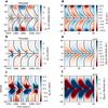 |
Fig. 5 Similar to Fig. 4 except that a simple decay of the poloidal and toroidal fields, with a decay time of 22 years, is included in the evolution equations for a and b, and a diffusivity η0 = 38 km2 s-1 is assumed in the bulk of the convection zone. |
Some of the quantities in these two formulae have been directly measured: Uθ,R⊙ = −27.9cosθsinθ + 17.7cos3θsinθ (Hathaway & Rightmire 2011); ΩR⊙ = 14.437−1.48cos2θ−2.99cos4θ (Hathaway & Rightmire 2011); and ΩRNSSL = 14.18−1.59cos2θ−2.61cos4θ + 0.53, following Schou et al. (1998) who give the surface rate and a near equator difference of 0.53°/day between the surface and bottom of the near-surface shear layer and Barekat et al. (2014), who report that the radial gradient at the top of the near-surface shear layer is independent of latitude.
The surface diffusivity ηR⊙ due to the advection of the surface field by the turbulent near-surface convective flows lies in the range of about 140 km2 s-1 to 600 km2 s-1 (Schrijver & Zwaan 2000). In previous studies we used a value of 250 km2 s-1, however, for this paper we found a slightly better match with the observations for ηR⊙ = 500 km2 s-1.
The source of poloidal flux as in the Babcock-Leighton framework is associated with Joy’s law and the emergence of active regions. We model it here as as = α0sinθcosθb(θ,t). For Vθ we chose the simplest functional form Vθ = V0sin(2θ). The parameters, ϵ, α0, and V0, are not directly given by observations. The effect of varying the parameters is discussed in Cameron & Schüssler (2017). The solutions are not very sensitive to the parameter ϵ, which lies in the range of 0 to 1, and we set it to 1 for this study (similar results can be found with ϵ = 0).
We chose α0 = 1 m s-1, V0 = 2 m s-1 and η0 = 90 km2 s-1 because these values (α0, η0, V0) give a reasonable correspondence of the model results to the observed azimuthally averaged radial and azimuthal field evolution, as can be seen in Fig. 4. The values used here seem plausible in comparison to the surface meridional flow of about 15 m s-1, and the subsurface diffusivity of mixing length theory.
The linear Eqs. (2)−(4) were solved numerically by discretizing the equations using a five point stencil and looking for the fastest growing eigensolutions. The match between the model and the observations, as shown in Fig. 4 is reasonable in the sense that the model captures most of the evolution of the large-scale field. Fine structure and cycle variability, introduced by the discreteness of emerge events, is beyond the scope of the model.
Our conclusion for this modeling part of the paper is that the updated Babcock-Leighton model presented in Cameron & Schüssler (2017) can explain important aspects of the observed evolution of the poloidal and azimuthal fields (including the extended solar cycle).
An important remaining issue is that the transport of average longitudinally averaged azimuthal flux through the solar photosphere during emergence reduces the subsurface toroidal field. To obtain an upper limit for the amount of flux lost, we consider that all of the toroidal flux calculated above as passing through the solar photosphere is lost to the interior. The average toroidal field strength of 0.1 G (from the ephemeral regions) carried across the entire solar surface with an average velocity of 1 km s-1 would carry 7.6 × 10²³ Mx of toroidal flux across the solar surface each 11 years. This should be compared with 2.4 × 1024 Mx of flux generated per (strong) cycle by the latitudinal differential rotation (Cameron & Schüssler 2015). The loss of toroidal field through the photosphere is therefore at most modest. In most flux transport dynamos, flux loss through the photosphere is included through a diffusive flux, which is consistent with the usually employed boundary condition where the toroidal field vanishes at the photosphere. In the original Babcock-Leighton formulation of Leighton (1969), this loss is treated with a simple decay term. In the formulation of Cameron & Schüssler (2017), used here, this loss term was ignored on the basis that the success of the surface flux transport model indicated that the decay timescale should not be less than a few cycles (Cameron et al. 2012). At such levels the decay term is not expected to produce qualitative changes in either the surface evolution of the radial field (Baumann et al. 2006) or the evolution of the subsurface toroidal field (Cameron & Schüssler 2015). To confirm this, Fig. 5 shows the result for a case where we included a simple loss term  and
and  with τ = 22 yr in Eqs. (3) and (5) and set η0 = 38 km2 s-1 such that the growth rate of the dynamo is positive but close to zero (all other parameters were the same as for Fig. 4). The results of this experiment are shown in Fig. 5. Including this flux loss, therefore, does not qualitatively affect our conclusions.
5. Conclusions
We have almost four cycles of observations of both the radial and azimuthal magnetic fields relevant for the global solar dynamo. To the extent that the solar dynamo is a cycle in which the poloidal field is generated from the toroidal field, followed by the generation of the toroidal field from the poloidal field, the observation of both these fields as a function of time and latitude, for almost four solar cycles, is a stringent constraint for dynamo models.
The (updated) Babcock-Leighton model is able to reproduce basic features of the observations with reasonable values of the free parameters of the model.
Acknowledgments
Data provided by the SOHO/MDI consortium. SOHO is a project of international cooperation between ESA and NASA. Wilcox Solar Observatory data used in this study were obtained via the web site http://wso.stanford.edu, courtesy of J. T. Hoeksema. NSO/Kitt Peak data used here are produced cooperatively by NSF/NOAO, NASA/GSFC, and NOAA/SEL. This work uses SOLIS data obtained by the NSO Integrated Synoptic Program (NISP), managed by the National Solar Observatory, which is operated by the Association of Universities for Research in Astronomy (AURA), Inc. under a cooperative agreement with the National Science Foundation.
References
- Altrock, R. C. 1988, in Solar and Stellar Coronal Structure and Dynamics, ed. R. C. Altrock, 414 [Google Scholar]
- Barekat, A., Schou, J., & Gizon, L. 2014, A&A, 570, L12 [NASA ADS] [CrossRef] [EDP Sciences] [Google Scholar]
- Baumann, I., Schmitt, D., & Schüssler, M. 2006, A&A, 446, 307 [NASA ADS] [CrossRef] [EDP Sciences] [Google Scholar]
- Cameron, R., & Schüssler, M. 2015, Science, 347, 1333 [NASA ADS] [CrossRef] [Google Scholar]
- Cameron, R. H., & Schüssler, M. 2016, A&A, 591, A46 [NASA ADS] [CrossRef] [EDP Sciences] [Google Scholar]
- Cameron, R. H., & Schüssler, M. 2017, A&A, 599, A52 [NASA ADS] [CrossRef] [EDP Sciences] [Google Scholar]
- Cameron, R. H., Schmitt, D., Jiang, J., & Işık, E. 2012, A&A, 542, A127 [NASA ADS] [CrossRef] [EDP Sciences] [Google Scholar]
- Carrington, R. C. 1858, MNRAS, 19, 1 [NASA ADS] [CrossRef] [Google Scholar]
- Centeno, R. 2012, ApJ, 759, 72 [NASA ADS] [CrossRef] [Google Scholar]
- Duvall, Jr., T. L. 1978, Ph.D. Thesis, Stanford Univ., CA [Google Scholar]
- Duvall, Jr., T. L., Scherrer, P. H., Svalgaard, L., & Wilcox, J. M. 1979, Sol. Phys., 61, 233 [NASA ADS] [CrossRef] [Google Scholar]
- Guglielmino, S. L., Martínez Pillet, V., Bonet, J. A., et al. 2012, ApJ, 745, 160 [NASA ADS] [CrossRef] [Google Scholar]
- Hagenaar, H. J. 2001, ApJ, 555, 448 [NASA ADS] [CrossRef] [Google Scholar]
- Hale, G. E., Ellerman, F., Nicholson, S. B., & Joy, A. H. 1919, ApJ, 49, 153 [NASA ADS] [CrossRef] [Google Scholar]
- Harvey, K. L. 1992, in The Solar Cycle, ed. K. L. Harvey, ASP Conf. Ser., 27, 335 [Google Scholar]
- Hathaway, D. H. 2015, Liv. Rev. Sol. Phys., 12, 4 [Google Scholar]
- Hathaway, D. H., & Rightmire, L. 2011, ApJ, 729, 80 [Google Scholar]
- Howard, R. 1974, Sol. Phys., 39, 275 [NASA ADS] [CrossRef] [Google Scholar]
- Jiang, J., Hathaway, D. H., Cameron, R. H., et al. 2014, Space Sci. Rev., 186, 491 [Google Scholar]
- Leighton, R. B. 1969, ApJ, 156, 1 [Google Scholar]
- Lo, L., Hoeksema, J. T., & Scherrer, P. H. 2010, in SOHO-23: Understanding a Peculiar Solar Minimum, eds. S. R. Cranmer, J. T. Hoeksema, & J. L. Kohl, ASP Conf. Ser., 428, 109 [Google Scholar]
- Martin, S. F., & Harvey, K. H. 1979, Sol. Phys., 64, 93 [NASA ADS] [CrossRef] [Google Scholar]
- McIntosh, S. W., Wang, X., Leamon, R. J., et al. 2014, ApJ, 792, 12 [NASA ADS] [CrossRef] [Google Scholar]
- Schou, J., Antia, H. M., Basu, S., et al. 1998, ApJ, 505, 390 [NASA ADS] [CrossRef] [Google Scholar]
- Schrijver, C. J., & Harvey, K. L. 1994, Sol. Phys., 150, 1 [NASA ADS] [CrossRef] [Google Scholar]
- Schrijver, C. J., & Zwaan, C. 2000, Solar and Stellar Magnetic Activity (Cambridge University Press) [Google Scholar]
- Schwabe, M. 1849, Astron. Nachr., 28, 302 [NASA ADS] [Google Scholar]
- Shrauner, J. A., & Scherrer, P. H. 1994, Sol. Phys., 153, 131 [NASA ADS] [CrossRef] [Google Scholar]
- Spörer, F. W. G. 1879, Astron. Nachr., 96, 23 [NASA ADS] [CrossRef] [Google Scholar]
- Ulrich, R. K., & Boyden, J. E. 2005, ApJ, 620, L123 [NASA ADS] [CrossRef] [Google Scholar]
- Wilson, P. R., Altrocki, R. C., Harvey, K. L., Martin, S. F., & Snodgrass, H. B. 1988, Nature, 333, 748 [NASA ADS] [CrossRef] [Google Scholar]
All Figures
|
Fig. 1 Surface longitudinally averaged azimuthal field determined from MDI (blue) and Wilcox Solar Observatory (red). The pink and light blue shadings show the formal error bars of the fittings. |
| In the text | |
|
Fig. 2 Simplified geometry of a flux emergence event. The tube (shown in red) has flux Φi. The spatial extent of the emergence, the separation of the footpoints, is L. During emergence, the tube crosses the photospheric layer Δz (shown in green) where the polarimetric magnetograph signal is formed. |
| In the text | |
|
Fig. 3 High-latitude (λ> 50°) surface longitudinally averaged azithmuthal field from WS0 (red) and polar (λ> 80°) surface longitudinally averaged radial field from KPNSO/VT (blue). The northern (southern) polar data are shown with the solid (dashed) curves. |
| In the text | |
|
Fig. 4 Time-latitude diagrams of the observed (left) and simulated (right) magnetic fields. Panel a: observed surface longitudinally averaged radial field based on KPNSO/VT and SOLIS data. Panel b: observed surface longitudinally averaged toroidal magnetic field based on WSO observations, and panel c is the same as panel b except saturated to bring out the weaker high-latitude fields. Panel d: surface radial field from the updated Babcock-Leighton model (Cameron & Schüssler 2017), panel e: subsurface toroidal flux density from the Babcock-Leighton model, and panel f shows a saturated version of panel e. The black lines in all the panels show the zero contours from the model. |
| In the text | |
|
Fig. 5 Similar to Fig. 4 except that a simple decay of the poloidal and toroidal fields, with a decay time of 22 years, is included in the evolution equations for a and b, and a diffusivity η0 = 38 km2 s-1 is assumed in the bulk of the convection zone. |
| In the text | |
Current usage metrics show cumulative count of Article Views (full-text article views including HTML views, PDF and ePub downloads, according to the available data) and Abstracts Views on Vision4Press platform.
Data correspond to usage on the plateform after 2015. The current usage metrics is available 48-96 hours after online publication and is updated daily on week days.
Initial download of the metrics may take a while.