| Issue |
A&A
Volume 608, December 2017
|
|
|---|---|---|
| Article Number | A83 | |
| Number of page(s) | 10 | |
| Section | Celestial mechanics and astrometry | |
| DOI | https://doi.org/10.1051/0004-6361/201731654 | |
| Published online | 11 December 2017 | |
Application of time transfer functions to Gaia’s global astrometry
Validation on DPAC simulated Gaia-like observations
1 INAF, Astrophysical Observatory of Torino, via Osservatorio 20, 10025 Pino Torinese (Torino), Italy
e-mail: This email address is being protected from spambots. You need JavaScript enabled to view it.
2 SYRTE, Observatoire de Paris, PSL Research University, CNRS, Sorbonne Universités, UPMC Univ. Paris 06, LNE, 61 avenue de l’Observatoire, 75014 Paris, France
3 Shanghai Astronomical Observatory, Chinese Academy of Sciences, 80 Nandan Road, 200030 Shanghai, PR China
4 EURIX SRL, via Giulio Carcano 26, 10153 Torino, Italy
Received: 26 July 2017
Accepted: 31 August 2017
Abstract
Context. A key objective of the ESA Gaia satellite is the realization of a quasi-inertial reference frame at visual wavelengths by means of global astrometric techniques. This requires accurate mathematical and numerical modeling of relativistic light propagation, as well as double-blind-like procedures for the internal validation of the results, before they are released to the scientific community at large.
Aims. We aim to specialize the time transfer functions (TTF) formalism to the case of the Gaia observer and prove its applicability to the task of global sphere reconstruction (GSR), in anticipation of its inclusion in the GSR system, already featuring the Relativistic Astrometric MODel (RAMOD) suite, as an additional semi-external validation of the forthcoming Gaia baseline astrometric solutions.
Methods. We extended the current GSR framework and software infrastructure (GSR2) to include TTF relativistic observation equations compatible with Gaia’s operations. We used simulated data generated by the Gaia Data Processing and Analysis Consortium (DPAC) to obtain different least-squares estimations of the full (five-parameter) stellar spheres and gauge results. These were compared to analogous solutions obtained with the current RAMOD model in GSR2 (RAMOD@GSR2) and to the catalog generated with the Gaia RElativistic Model (GREM), the model baselined for Gaia and used to generate the DPAC synthetic data.
Results. Linearized least-squares TTF solutions are based on spheres of about 132 000 primary stars uniformly distributed on the sky and simulated observations spanning the entire 5 yr range of Gaia’s nominal operational lifetime. The statistical properties of the results compare well with those of GREM. Finally, comparisons to RAMOD@GSR2 solutions confirmed the known lower accuracy of that model and allowed us to establish firm limits on the quality of the linearization point outside of which an iteration for non-linearity is required for its proper convergence. This has proved invaluable as RAMOD@GSR2 is prepared to go into operations on real satellite data.
Key words: astrometry / gravitation / methods: data analysis / space vehicles: instruments
Present address: Astronomical Institute, University of Bern, Sidlerstrasse 5, 3011 Bern, Switzerland.
© ESO, 2017
1. Introduction
The Gaia space satellite, operational since 2014, performs 4π (steradians) absolute astrometry, aiming at the definition of a global astrometric reference frame at visual wavelengths to unprecedented accuracies. Within this context, it will be very difficult to identify possible errors in the measurements or in the data reduction process by using external comparisons of similar accuracies across the sky as they are simply not available. For this reason, beside the main processing pipeline, the Gaia Data Processing and Analysis Consortium (DPAC) has established an astrometric verification unit (AVU) to verify crucial steps in the baseline data processing chain and report on any significant difference (Vecchiato et al. 2012). This step is essential in order to guarantee a high quality catalog to the larger scientific community.
Moreover, the processing of astrometric observations at the μas (micro-arcsecond) accuracy required by the Gaia mission demands to take into account relativistic effects on clock synchronization, reference frame transformations as well as on light propagation. Indeed, the behavior of electromagnetic waves (EW) in the solar system is highly sensitive to space-time curvature. Most of the available models are based on the solution of null geodesic equations, including those currently used to process Gaia observations: Gaia RElativistic Model (GREM; Klioner 2003) for the main processing pipeline of the Astrometric Global Iterative Solution (AGIS; Lindegren et al. 2012) and the Relativistic Astrometric MODel family (RAMOD; Crosta et al. 2017, 2015, and references therein) for the AVU as implemented in the Global Sphere Reconstruction (GSR; Abbas et al. 2011) subsystem hosted at the Italian Data Processing Center in Torino (DPCT, Messineo et al. 2012).
Nevertheless, other approaches exist, such as the one first based on the Synge World Function (Le Poncin-Lafitte et al. 2004) and then improved with the use of the time transfer functions (TTF; see Teyssandier & Le Poncin-Lafitte 2008). Similarly to the other methods this approach provides “ready-to-use” analytical formulas to describe light propagation in the field of multiple axisymmetric bodies moving with arbitrary velocities in the post-Minkowskian framework (Hees et al. 2014a) and up to the second and third order for static perturbing bodies (Linet & Teyssandier 2013; Hees et al. 2014b). The equivalence of the TTF approach has been verified analytically with RAMOD in the static case and with GREM in the case of slowly moving monopoles (Bertone et al. 2014). However, equivalence on the analytical side does not guarantee equivalence of the numerical results (Vecchiato et al. 2014).
The task of providing the best possible confidence in the data reduction process is precisely the main responsibility of AVU. To this aim, having the possibility of reducing data with different approaches would surely increase the level of reliability from the point of view of the theoretical understanding of the data.
In this paper, we present results of the first application of the TTF approach to global astrometry in the framework of the Gaia mission, which is preparatory to its successive inclusion in the AVU/GSR operational infrastructure next to the models of the RAMOD family. In Sect. 2 we briefly recall the astrometric problem of processing Gaia observations and how it is addressed in GSR. In Sect. 3 we present our new implementation, GSR-TTF, by first describing how the TTF equations have been integrated in the GSR modeling of Gaia observations at the required accuracy. Then, we provide the equations of the coefficients required for the least-square solution of the sphere. We take advantage of the modularity of the GSR software infrastructure, which allows for an easy plugin of, for example, light propagation equations and reference frames transformations. Finally, we present in Sect. 4 the comparison of our modeling to the GREM implementation in GaiaTools (ter Linden & GaiaTools Committee 2009; Balm & GaiaTools Committee 2014) as well as solutions of a sphere of about 132 000 stars based on DPAC simulated data. Section 5 suggests possible developments and further applications for the results presented in this work and our concluding remarks.
2. The astrometric problem in GSR
2.1. Astrometric coordinates in Gaia
As shown in Fig. 1, each point of the celestial sphere can be fixed in the reference frame of the Gaia spacecraft by three direction cosines defined as  (1)with i = 1,2,3.
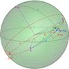 |
Fig. 1 Fundamental angles in the Gaia reference frame Eâ. The two Fields of View (FoV) directions are indicated by f+ and f− while the measured abscissa is given by n(i) = (α,β,δ) (from Vecchiato et al. 2012). |
From a geometrical point of view, Gaia measures the abscissa φ and the ordinate ζ, also called along-scan (AL) and across-scan (AC) coordinate, of such a point. In particular, the AL coordinate is the angle φ between the x-axis of the spacecraft, denoted Ex in Fig. 1, and the projection of the point along the great circle traced by the Ex and Ey axes, which identifies the instantaneous scanning direction of the satellite. The angle φ is related to the direction cosines n(i) by the following relations  As illustrated in Gaia Collaboration (2016) and Perryman et al. (2001), the Gaia spacecraft has two fields of view (FoV) called f+ and f− whose pointing directions are separated by a fixed base angle of Γ = 106.5° and which are symmetric with respect to the x-axis. Since the angular amplitude of each FoV is about 0.5°, the abscissae range is fixed in the intervals 53.25 ± 0.25 deg for f+ and −53.25 ± 0.25 deg for f−. Therefore, one of Eqs. (2)is enough to determine a univocal correspondence between the value of φ and that of the direction cosines. Gaia’s measurement is three times more sensitive in the AL direction than in the across one, so, in principle, the cosφ observation equation is sufficient to solve the sphere problem, which is what we have done in this paper; however, since to first order the abscissa measurement is independent from the orientation of the Ez axis, one should also build an observation equation using the AC measurement ζ to better constrain the attitude when the latter is being reconstructed along with the astrometric parameters. The abscissa is generally expressed as function of the astrometric parameters (namely, the right ascension α∗, declination δ∗, parallax ϖ∗, and proper motions μα ∗ and μδ ∗) and of the satellite attitude
  , where the index j refers to the time of observation, and i to the number of parameters used to model the attitude. The latter has to be considered unknown since the satellite attitude cannot be determined by other independent measurements at the accuracy required by the mission. For a similar reason Eq. (2a)also depends on a set of instrument parameters { cl } to provide a sort of long-term calibration. Moreover, when working within the parametrized post-Newtonian (PPN) formalism, one should add the parameter γ to the unknowns. A better determination of γ, which measures the amount of curvature induced by the mass-energy on space-time, shall be one of the important scientific contributions of Gaia (Perryman et al. 2001). As consequence, each AL observation can be modeled by a non-linear function of these four classes of unknowns, as
  (3)
(3)
2.2. The GSR approach to the processing of observations
The Gaia mission will perform several billion observations during its operational years, so that the problem of the so-called sphere reconstruction translates into the solution of a very large system of equations (up to 1010 × 108 in the case of Gaia). Solving such a big system of non-linear equations is not feasible, so the observation Eq. (3)are linearized about a convenient starting point, that is, the current best available estimate of the required unknowns. The problem is then converted in a corresponding system of linear equations 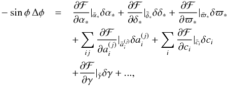 (4)where the unknowns are the corrections δx to the a-priori values (e.g., from stellar catalogs) while the derivatives of ℱ are the coefficients of the design matrix. The known-terms are then represented by the left-hand side of Eq. (4)as
  (5)where φobs represents the observed abscissa and formally includes the measurement errors so that it can be written as φobs = φtrue + Δφ, while φcalc is the computed value given by arccos(ℱ) at the starting point of the linearization (generally speaking, the value contained in the astrometric catalog).
The resulting system of equations is quite sparse since each observation refers to a single star among the millions considered in the reconstruction problem (and then only to its astrometric parameters). A similar reasoning is valid for the attitude and calibration parameters, while γ is a global parameter in the sense that it appears in each equation of the system. The number of observations being far larger than the number of unknown parameters, the system is over-determined and can be solved by a least-squares procedure. The final goal of the entire procedure is then to get better estimates of all the intervening parameters but for that, we first need to provide an accurate model of the direction cosines of the observation.
The input of the code are packets, each containing observations characterized by: the coordinate time of observation (necessary to retrieve Gaia state vector and the planetary ephemerides at the appropriate epoch), the catalog coordinates of the observed source and all quantities used in the setup of the observation equations for the astrometric problem, which we are going to detail in the following. The values contained in the packet are then updated by the processing of the observation. For each of the processed observations the following steps are performed:
-
Load the observations packets and launch the analysis routines;
-
Call, for each observation, the routines defining all needed quantities for the computation of the astrometric observable;
-
Define all needed vectors (star-observer, perturbing body-observer, ...) and tensors (tetrad components, metric, ...);
-
Define φobs and φcalc, compute the known-terms (5);
-
Compute the coefficients of the linearized observation Eq. (4);
-
Coefficients and known-terms are associated to an observation and stored in a packet to be then used for the setup of the observation equation and the astrometric solution in a least-squares sense.
The GSR software has been conceived to be as neutral as possible with respect to the astrometric model. In particular, as long as the latter agrees with some given input and output specifications, one can plug-in any relativistic model, which is seen as a black box by the pipeline. In the current version of GSR (GSR2, see Sect. 4) the direction cosines are provided using a relativistic model from the RAMOD family (more precisely, the version actually implemented in the operational infrastructure at DPCT is RAMOD@GSR2, Vecchiato et al., in prep.), but the modular structure of the software makes it easy to produce a GSR-compatible implementation of the TTF astrometric model, which we denote as GSR-TTF.
3. TTF implementation in GSR
The goal of this work is to setup the processing of astrometric observations (eventually made by Gaia) using the TTF formalism. To do it, we implement our model in the GSR software developed at Turin Observatory and we use it to generate a series of simulated observations. The result is a “GSR-TTF plug-in” which enables the pipeline to reduce the sphere with another model, which is actually more accurate than the RAMOD@GSR2 one. The TTF model can, in fact, be implemented at several different level of accuracy. We decided to limit the present one to a (v/c)3 version at the same level of GREM, where v is the velocity of the observer with respect to the Barycentric Celestial Reference System (BCRS). This allows to neglect all the complications coming from higher-orders of v/c and to non-spherically symmetric gravity fields, which are deemed negligible for the specific problem of the global sphere reconstruction. The implementation of the astrometric observable in GSR concerns the development of both sides of Eq. (4), as we detail in this section.
3.1. Setup of the observation abscissae
Let us show the procedure followed to build the abscissa φ using our astrometric model. First, following the definition of astrometric observable in the tetrad formalism (Brumberg 1991) given by Hees et al. (2014b), we define the direction cosines appearing in Eq. (2a), taken at the observation point xB as  (6)where we shall choose the direction triple
  (defining the barycentric direction of light) and the tetrad
  (i.e., the transformation matrix to the reference system comoving with the observer) according to the accuracy required by the Gaia mission.
The relations between the TTF and the wave vectors kμ = dxμ/ dλ at reception have been derived in Le Poncin-Lafitte et al. (2004) as ![Mathematical equation: \begin{equation} \left(\widehat{k}_i\right)_B = \left(\frac{k_i}{k_0}\right)_B = -c \, \frac{\partial {\cal T}_{\rm e}}{\partial x^{i}_{B}} \, = \, - c \, \frac{\partial {\cal T}_{r}}{\partial x^{i}_{B}} \left[1 - \frac{\partial {\cal T}_{r}} {\partial t_B}\right]^{-1} \cdot \label{eq:k} \end{equation}](/articles/aa/full_html/2017/12/aa31654-17/aa31654-17-eq51.png) (7)We put xA = (ctA,xA), the event of emission
(7)We put xA = (ctA,xA), the event of emission  and xB = (ctB,xB), the event of reception ℬ of a light signal. Moreover, we define
  and
and  as two distinct (coordinate) TTF defined as
  (8)where
  and
and  are evaluated at the event of emission and at the event of reception ℬ respectively. For astrometric applications, we are only interested in .
For applications in the solar system, we can work in the weak field approximation so that we can write  (9)with ημν = diag(−1, + 1, + 1, + 1) a Minkowskian background and hμν a small perturbation. Moreover, we shall consider only weak gravitational fields generated by self-gravitating extended bodies within the slow-motion, post-Newtonian approximation. So, we assume that the potentials hμν may be expanded as
 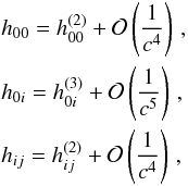 (10)where
  ,
,  and U is the Newtonian potential.
Under these hypotheses, the expression of the TTF  in the PPN approximation has been given in Linet & Teyssandier (2002) and in Teyssandier et al. (2008) as
  (11)where Δr is defined as
 ![Mathematical equation: \begin{equation} \Delta_{r} = \frac{1}{2}R_{AB}\int_{0}^{1}\left[h^{(2)}_{00} + 2 N_{AB}^{i} h^{(3)}_{0i} + N_{AB}^{i} N_{AB}^{j} h^{(2)}_{ij}\right]_{z^\alpha_{-}(\lambda)} {\rm d}\lambda \label{Tr1wIAUs} , \end{equation}](/articles/aa/full_html/2017/12/aa31654-17/aa31654-17-eq71.png) (12)and the integrals are taken along the Minkowskian paths
(12)and the integrals are taken along the Minkowskian paths  and we define
  ,
,  and
and  .
.
The derivatives needed in the definition of the wave vectors in Eq. (7)can then be computed as (see, e.g., Bertone et al. 2014; Hees et al. 2014b,a)  (13a)and
  (13b)where
 ![Mathematical equation: % subequation 1514 0 \begin{equation} \label{eq:dDr1PM} \frac{\partial \Delta_r }{\partial x^i_B} = -\frac{1}{2} \int_0^1 \left[ R^i_{AB} \lambda m_{,0} - R_{AB} (1-\lambda) m_{,i} - \tilde h_i \right]_{z_-^\alpha (\lambda)} {\rm d}\lambda , \end{equation}](/articles/aa/full_html/2017/12/aa31654-17/aa31654-17-eq78.png) (14a)and
(14a)and ![Mathematical equation: % subequation 1514 1 \begin{equation} \frac{\partial \Delta_r }{\partial t_B} = c \frac{R_{AB}}{2} \int_0^1 \left[ m_{,0} \right]_{z_-^\alpha (\lambda)} {\rm d}\lambda . \end{equation}](/articles/aa/full_html/2017/12/aa31654-17/aa31654-17-eq79.png) (14b)Moreover, we defined
(14b)Moreover, we defined  For most observations, at Gaia accuracy we shall only consider the PN gravitational potentials of all solar system bodies as point masses. Quadrupole terms might be significant for a limited number of observations grazing giant planets (e.g., closer than 152′′ from Jupiter’s limb at 1 μas accuracy Klioner 2003; Crosta & Mignard 2006), hence we are including them in our implementation.
Also, it has been shown (Vecchiato et al. 2003) that thanks to the satellite’s high measurement accuracy, the Gaia sphere reconstruction is sensitive to variations of the γ parameter of the PPN formalism up to the 10-6–10-7 level. This processing can thus be used as a tool to improve our knowledge of such parameter, which is currently set at the 10-5 level (Will 2014). With this application in mind γ can be straightforwardly introduced by using the PPN expression of the above metric coefficients hαβ, where  and wP(t) is the time-dependent gravitational potential of perturbing body P. This time-dependence would in principle require either to express w as a retarded potential, or to compute a full integral of the geodesic. However, it has been shown in Klioner (2003) and confirmed by our analysis in Bertone et al. (2014), that at the Gaia accuracy the effects of a time-dependent perturbation due to a moving body can be taken into account simply by computing the positions of the gravitating bodies at the retarded moment of time
  (18)where tB is the coordinate time of observation and xP(tB) is the position of body P at tB, and that the “gravitomagnetic” contributions proportional to vP(t) can be neglected.
Thus, using such constant value xP = xP(tC) in our computations yields to the following expression of the PN terms of the metric tensor:  Let us assume that the smallest sphere containing the body has a radius equal to the equatorial radius re of the body and that the segment joining xA and xB is outside this sphere. Also, let us restrict to the case of axisymmetric perturbing bodies with time-independent mass-multipoles. At any point x such that r ≥ re, the gravitational potentials w and w are then given (for each body P) by the multipole expansion (Linet & Teyssandier 2002)
 ![Mathematical equation: \begin{equation} \label{eq:gravpotmultip} w_P = \frac{G {\cal M} }{r_P}\left[1 - \sum_{n=2}^{\infty} J_n \left(\frac{r_{\rm e}}{r_P}\right)^n P_n \left(\frac{\bk .\bx}{r_P}\right)\right] \quad \mbox{and} \quad \bm w_P =0 , \end{equation}](/articles/aa/full_html/2017/12/aa31654-17/aa31654-17-eq103.png) (20)where
(20)where  (21)k denotes the unit vector along the x3-axis, the Pn are the Legendre polynomials, ℳ is the mass of the body and the coefficients Jn are its zonal spherical harmonics coefficients.
Under these assumptions, the monopolar and quadrupolar terms of the direction triple to be used in Eq. (6)are (Le Poncin-Lafitte & Teyssandier 2008; Bertone et al. 2013) ![Mathematical equation: % subequation 1724 0 \begin{eqnarray} (\hat k_i^B)(\bx_A,\bx_B) &=& \nabi - (\gamma+1) \sum_P \frac{G {\cal M}_P}{c^2 R_{PB}}\, \frac{1}{1 + \bN_{PA} \cdot \bN_{PB}} \nn\\&&\quad \times \left[\frac{R_{AB}}{R_{PA}}\bN_{PB} -\left(1 + \frac{R_{PB}}{R_{PA}}\right)\bN_{AB}\right] , \label{M0} \end{eqnarray}](/articles/aa/full_html/2017/12/aa31654-17/aa31654-17-eq110.png) (22a)
(22a)![Mathematical equation: % subequation 1724 1 \begin{eqnarray} (\hat k_i^B)_{J_2}&&(\bx_A,\bx_B) = (\gamma +1)\frac{GM}{c^2} J_2 r_{\rm e}^2 \Bigg\lbrace - \Big[ \bk \cdot (\bN_{PA} + \bN_{PB}) \Big]^2\nn\\ && \times \left[\frac{\bN_{PB} - \bN_{AB}}{(R_{PA}+R_{PB}-R_{AB})^{3}}- \frac{\bN_{PB} + \bN_{AB}}{(R_{PA}+R_{PB}+R_{AB})^{3}}\right] \label{M2} \nonumber \\ && \nn \\ && +\frac{1}{2}\left[\frac{1-(\bk \cdot \bN_{PA})^2}{R_{PA}} + \frac{1-(\bk \cdot \bN_{PB})^2}{R_{PB}}\right] \nn\\ && \times\left[\frac{\bN_{PB} - \bN_{AB}}{(R_{PA}+R_{PB}-R_{AB})^{2}} - \frac{\bN_{PB} + \bN_{AB}}{(R_{PA}+R_{PB}+R_{AB})^{2}}\right] \nonumber \\ && +\frac{1}{R_{PB}^3}\frac{(R_{PA} + R_{PB})R_{AB}}{R_{PA}^{2}}\frac{\bk . (\bN_{PA} + \bN_{PB})}{(1 + \bN_{PA} \cdot \bN_{PB})^2} \nn\\ && \times \Big[ \bk - (\bk \cdot \bN_{PB})\bN_{PB} \Big] \\ && +\frac{1}{2 R_{PB}^3}\frac{R_{AB}}{R_{PA}}\frac{2(\bk \cdot \bN_{PB})\bk + \left[1 - 3(\bk \cdot \bN_{PB})^2\right]\bN_{PB}}{1 + \bN_{PA} \cdot \bN_{PB}}\Bigg\rbrace \nn , \end{eqnarray}](/articles/aa/full_html/2017/12/aa31654-17/aa31654-17-eq111.png) (22b)respectively, and where we used
(22b)respectively, and where we used  An expression for the multipolar terms of higher order is given in Le Poncin-Lafitte & Teyssandier (2008) but it is not relevant for this study.
The direction triple  , defined as the sum of Eqs. (21a) and (21b), gives the direction of the light ray at reception in the local barycentric frame. Following Eq. (6), we hence need to project this vector in the observer reference frame. Concerning this point, we have used the tetrad defined in Crosta & Vecchiato (2010) and already used in GSR, evaluated with the same metric (Eq. (18)).
The satellite reference frame defining the transformation  is obtained by successive transformations of the local BCRS tetrad (Bini et al. 2003)
  (24)namely the tetrad obtained from the BCRS by shifting the origin to the instantaneous barycenter of the satellite. This tetrad, and in particular the triad of four-vectors λâ defined as the spatial part of
  , is “boosted” to the satellite rest-frame by means of an instantaneous Lorentz transformation identified by the four-velocity of the observer
  with respect to the local BCRS. The boosted tetrad
  , namely (Crosta & Vecchiato 2010)
  (25)obtained in this way represents a reference system whose origin is comoving with the barycenter of the satellite and whose spatial axes are kinematically non-rotating with respect to the BCRS. The Gaia attitude frame is finally obtained with a rotation of these spatial axes. Since the transformation is Euclidean, the rotation matrix A is exactly the attitude matrix of the satellite.
The triad resulting from these transformations, detailed in Crosta & Vecchiato (2010), establishes the Gaia relativistic attitude triad and is related to the euclidean attitude parameters by  (26)The temporal axis of the tetrad has to be transformed alike to obtain a complete reference system attached to the observer. This result is naturally achieved by writing the transformation between the barycentric coordinate time and the observer’s proper time.
Finally, introducing Eq. (6)into Eq. (2a)completes the implementation in the observation abscissa of GSR-TTF.
3.2. Setup of the astrometric coefficients
In order to setup the observation equation for the improvement of the a priori catalog values by a least-square procedure, we define the partial derivatives of Eq. (3)w.r.t. the astrometric parameters as in Eq. (4). The coefficients can be computed analytically since the function ℱ = cosφcalc, defined by Eq. (2a), is known. By defining n(i) = cosψ(i), the coefficients of Eq. (2a)can be computed analytically as  (27)where v are the so called astrometric parameters characterizing the coordinates of a star at a moment in time: the parallax ϖ∗, right ascension α∗, declination δ∗, and the proper motions μα∗ and μδ∗ in perpendicular directions. The partial derivatives appearing therein are given by
 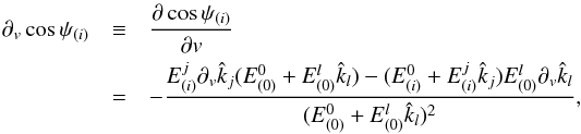 (28)with
 ![Mathematical equation: \begin{eqnarray} \frac{\partial \hat k_i}{\partial v} &=& \partial_v \nabi - (\gamma + 1) \sum_P \frac{G {\cal M}_P}{c^2 \rpb} \frac{1}{1+ \bnpa \cdot \bnpb}\nn \\ &&\quad \times \Bigg\{ - \frac{\partial_v \bnpa \cdot \bnpb}{1+ \bnpa \cdot \bnpb} \times \Bigg[ \nabi \frac{\rab}{\rpa} - \nabi \Bigg(1 + \frac{\rpb}{\rpa}\Bigg) \Bigg] \nn \\ &&\quad +\frac{N_{PB}^i}{\rpa^2} \Big(\rpa \partial_v \rab - \rab \partial_v \rpa \Big) \nn \\&& \quad - \partial_v \nabi \Bigg(1+\frac{\rpb}{\rpa} \Bigg) + \nabi \rpb \frac{\partial_v \rpa}{\rpa^2} \Bigg\} \cdot \end{eqnarray}](/articles/aa/full_html/2017/12/aa31654-17/aa31654-17-eq130.png) (29)Moreover, we used the definitions (22)along with
(29)Moreover, we used the definitions (22)along with ![Mathematical equation: % subequation 1951 0 \begin{eqnarray} \partial_v \nabi &=& - \frac{(\bnab \times (\partial_v \bx_A \times \bnab) )^i}{\rab} , \\ \partial_v \rab &=& - \frac{\bm \rab \cdot \partial_v \bx_A}{\rab} , \\ \partial_v \rpa &=& \frac{\brpa \cdot \partial_v \bx_A}{\rpa} , \\ \partial_v \bnpa &=& \frac{1}{\rpa} \Big[ \partial_v \bx_A - \bnpa (\bnpa \cdot \partial_v \bx_A) \Big] , \end{eqnarray}](/articles/aa/full_html/2017/12/aa31654-17/aa31654-17-eq131.png) where × indicates a cross-product. The expression in terms of the astrometric parameters can be easily obtained by considering that the coordinate position of the source xA(t) can be treated like a Euclidean vector, so that xA(t) = (rAcosα(t)cosδ(t),rAsinα(t)cosδ(t),rAsinδ(t)), where rA = | xA | is the barycentric distance of the star, ϖ ≡ 1UA/rA. Finally, the angular coordinates α(t) and δ(t) at a given time t can be expressed as functions of the catalog positions and proper motion with, for example, α(t) = αt0 + μα∗dt, dt being the interval of time between t and the catalog reference time t0. We can thus write
where × indicates a cross-product. The expression in terms of the astrometric parameters can be easily obtained by considering that the coordinate position of the source xA(t) can be treated like a Euclidean vector, so that xA(t) = (rAcosα(t)cosδ(t),rAsinα(t)cosδ(t),rAsinδ(t)), where rA = | xA | is the barycentric distance of the star, ϖ ≡ 1UA/rA. Finally, the angular coordinates α(t) and δ(t) at a given time t can be expressed as functions of the catalog positions and proper motion with, for example, α(t) = αt0 + μα∗dt, dt being the interval of time between t and the catalog reference time t0. We can thus write 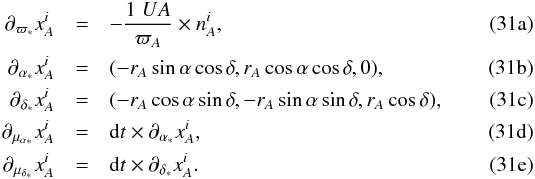 The system is then solved following a classical least-squares method.
3.3. Setup of the global PPN parameter γ
Following a similar approach, we computed and implemented the partial derivatives of the astrometric observable with respect to the global PPN parameter γ, which can be used to test General Relativity using light propagation measurements.
Considering Eq. (27), we have that both the tetrad  and the direction triple
  depend on γ through the metric (18). Hence we get
 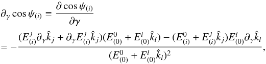 (32)and, with Eqs. (21), (25)and (26),
 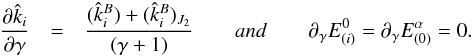 (33)
(33)
4. GSR-TTF: results with Gaia simulated observations
Our implementation is tested by using observations of the Gaia satellite as simulated by DPAC using the GREM model. In particular, the dataset employed is RDS-7-F (Luri et al. 2010), a full 5 yr simulation of Gaia observations of two million stars, approximately one million of which are Primary astrometric sources in the sense discussed in Lindegren et al. (2012). Besides the noise-free measured GREM abscissa η (see Eq. (34)below), the data set provides: stellar coordinates, observation epoch, instantaneous satellite attitude, and the ephemerides of the solar system. These data allow us to compute the abscissa φ from a given model. As for the observation error, this can be customized. In our experiments all stars have Gaia magnitude G = 14, and at such brightness the expected single observation error is σ0 = 125μas.
The TTF model is therefore tested in two steps: by comparing the abscissae (2a)computed by TTF and GREM, and by trying some reconstructions of the global astrometric sphere. The latter had to be restricted to relatively small subsamples of stars and observations in RDS-7-F. This is because only limited resources are allocated to the test & development section of the GSR system at DPCT, the environment for running experiments with simulated data.
4.1. Numerical comparison of computed observables
As anticipated above, we first focused on the comparison of the abscissa φ. Using the implementation described in Sect. 3.1, we applied Eq. (2a)over a set of observations from a chosen day of the given dataset using the TTF model, thus obtaining φTTF. The same data are used with the tools provided by the DPAC code, which implements the GREM model, to obtain φGREM. Finally, the residuals φTTF−φGREM were computed.
The results are illustrated in Fig. 2, where the models are compared. The left axis marks the difference in μas between the two models while the right axis is the angular distance in degrees between a given planet and the observation, namely its elongation. Lines representing Jupiter, Saturn, and the Earth are all plotted. In particular, the periodic oscillation of the distance planet-observation illustrated in the plots is due to the Gaia scanning law (de Bruijne et al. 2010) setting a rotation period of approximately 6h.
As expected from the analytical comparisons in Bertone et al. (2013) and Bertone et al. (2014), the plot shows that the differences between the abscissae computed with the two models are generally well below ± 1μas. The remaining sub-μas signal can be attributed to a different accounting of the retarded times in Eq. (18)or to differences in the representation of satellite attitude.
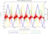 |
Fig. 2 Difference between the abscissae resulting from the GSR-TTF implementation and from GREM implementation in the “GaiaTools”. The left axis indicates the difference in μas between the two models – represented by the red plot; the right axis indicates the distance in degrees between a given planet and the observation – the blue, yellow and green plot representing Jupiter, Saturn and the Earth, respectively. |
The final accuracy of a global sphere reconstruction depends on the statistical properties of the model accuracy, in the sense that possible inaccuracies affecting some observations because of its specific geometric arrangement are likely to get “blended” and “smoothed out” by other, more accurate observations featuring a more benign configuration. It is therefore appropriate to give also a statistical assessment of these differences. Figure 3 shows the distribution of abscissae differences for observations taken over a period of 40 days. The vast majority of the differences are in the range ± 0.2 μas.
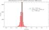 |
Fig. 3 Abscissae differences between the GSR-TTF and GREM implementations. The vast majority of the observations show differences in the interval of ± 0.2 μas, well below the accuracy required by Gaia. |
4.2. Application to the reconstruction of the celestial sphere
The main goal of the Gaia mission is to improve the quality of the stellar catalogs for coordinates, parallaxes and annual proper motions of the observed stars. This is done by evaluating the differences between the high-precision angular measurements made by the satellite and their analytical modeling as functions of the astrometric stellar parameters. As described in Sect. 2.2, this is essentially a minimization problem obtained by solving a large and sparse system of linearized observation equations in the least-squares sense. Indeed, the problem is largely over-determined (Gaia will provide around 700 observations for each star, see e.g. Mignard et al. 2008, or Fig. 4) which justifies the least-squares solution of the equation system.
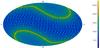 |
Fig. 4 Frequency of observations as function of celestial coordinates due to Gaia scanning law (blue ≈50 – yellow ≈500). |
Our implementation is then tested by using observations of the Gaia satellite simulated with the GREM model, as a replacement of the real Gaia observations, and the TTF model. In particular, for each observation it is possible to compute the true AL field angle η. Then, by definition, the abscissa of Eq. (2a)can be expressed as  (34)where Γ, as shown in Fig. 1, is the basic angle, that is the angle between the axes of the preceding and following FoV, and f = ± 1 with sign determined by the FoV in which the star is observed. In particular f takes the minus sign in the case of f−, and the positive one for f+.
The abscissae defined in this way are the values of φobs in Eq. (5), while φcalc is given by the TTF model. This allows the computation of the known term of the linearized observation equation. Such an equation is completely set up by computing the first order derivatives with respect to the unknown parameters, as described in Sect. 3.2, for which we still need to define the linearization point. Finally, measurement errors must also be introduced in each observation equation.
Specifically, the observed abscissa φobs produced from the dataset should represent the value of a measurement. However, the simulated dataset provides us with the true values, in the sense specified above, that is, the GREM model is supposed to give the correct physical representation of light propagation. Moreover, the coefficients of the linearized equation are computed at specific values, which are our best estimation of the unknowns. Once again, the input catalog provides the true values, while in a more realistic situation one should take into account that our initial guesses will be perturbed by some catalog error. The worse these errors, the larger are the linearization errors which will eventually affect the solution. The above discussion, therefore, makes it clear why in our tests we follow a procedure in three steps:
-
1.
we use the true catalog values to simulate both Gaia“measurements” (φobs) and compute the right-hand-side of Eq. (4). This is equivalent to assume no measurement or catalog error on our a-priori information and allows us to test the reliability of our model (see Col. 0101 in Table 1);
-
2.
we apply a random Gaussian error (μ = 0, σo = 125 μas) to φobs, but we use the true values for φcalc and for the coefficients. This simulates the impact of the measurement error on the quality of the updated catalog (see Col. 0102 in Table 1), but minimizes the linearization errors on the final solution;
-
3.
in addition to the above measurement error, we apply a Gaussian noise of σ = 20 mas to the catalog values. This introduces a contribution to the final solution due to the linearization errors of Eq. (4)(see Col. 0301 in Table 1).
We emphasize that these kind of runs are only testing the applicability of the TTF model in the case of the estimation of the astrometric parameters. The actual case of a Gaia-like mission, the attitude parameters have to be estimated as well within the global sphere reconstruction. This is because neither the usual instrumentation for the on-board attitude reconstitution nor a short-term astrometric determination can provide a sufficiently good reconstruction, given the measurement accuracy. In this proof-of-principle, however, the main goal is to test the applicability of TTF; therefore, as a first step, it is required that we compare its accuracy with that of the Gaia baseline model GREM treating the attitude as perfectly known.
We therefore applied this procedure to a subset of RDS-7-F, namely, to 132 000 stars homogeneously distributed on the sky for which the five years of the planned mission provide ~92 400 000 individual observations.
The final goal of the procedure is to retrieve as much as possible the catalog values for the estimated parameters of the 132 000 processed stars. We evaluated the quality of the estimation simply by computing the residuals of the updated minus true astrometric parameters (separately for each of the five) and afterwards by calculating their average and σ.
If the two models gave exactly the same value of the abscissae, and allowing an infinite machine precision, in the 0101 case we would expect exactly a zero solution. Since computers have a finite computing precision, and numerical errors tend to cumulate, even if the first condition would be met one should expect deviations from this solution larger than the machine precision, which in our case is about 10-16. Such numbers have to be interpreted as radians, which implies that deviations cannot be smaller than 10-4μas. Moreover, the different numerical predictions of the two models, if present, can show up both as random errors and systematic biases in the TTF reconstruction, namely in non-negligible σ and averages respectively. Within Gaia’s astrometric tolerances, the two models are equivalent if in such test one obtains sub-μas values for these two quantities.
In the 0102 case we introduced a purely Gaussian measurement error, which should decrease with  , where nobs is the number of observations of a particular star. In fact, when the attitude is assumed perfectly known, along with the instrumental and global parameters, each star is completely independent from all the others, and the complete system is indeed equivalent to a set of independent systems, one for each star. Figure 5 confirms the expected behavior of the residuals for each parameter and each star. Considering that Gaia is going to measure each star about 700 times, on average, and that there are five astrometric parameters, one can roughly estimate that
  (35)Finally, in the 0301 case, we have to consider the effect of the linearization errors. It is well known that, as long as the initial guess provided by the catalog is sufficiently close to the true values, this test should give the same result of the 0102 case. It is implicit that the expression “the same result” must be intended in the numerical sense, that is “the same with respect to the required accuracy”, which in the Gaia case means to the sub-μas level.
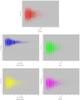 |
Fig. 5 Astrometric post-fit residuals for a set of 132 000 stars as function of the number of observations for each star (red: ϖ, blue: αcosδ, green: δ, yellow: μαcosδ, purple: μδ) . |
Results with GSR-TTF applied to 5 yr of observations of 132 K stars homogeneously distributed on the sky (in μas and μas / yr).
Results with RAMOD@GSR2 applied to 5 yr of observations of 132 K stars homogeneously distributed on the sky (in μas and μas / yr).
Table 1 shows the results of these tests, while Fig. 6 shows the post-fit residuals distribution for all astrometric parameters. Therefore, for what concerns the astrometric unknowns, we can conclude that the GREM and TTF models are equivalent. Moreover, TTF is able to recover these parameters down to the expected level of accuracy. Finally, starting from a reasonable catalog error the same astrometric accuracy can be recovered at the sub-μas level.
Table 2 reports the results of analogous runs on the same simulated datasets, but this time obtained using the RAMOD@GSR2 model, the one operational in the current version of the GSR system (GSR2) at DPCT. Runs 0101 and 0102 compare reasonably well with the corresponding ones of TTF, although the sub-μas level of the average residuals already reveals the expected intrinsic lower accuracy of the RAMOD@GSR2 model. The discrepancies appearing in run 0301, the one reflecting the real case scenario, are significant at the μas level and we carefully addressed their origin.
The ultimate reason of this discrepancy is actually non-linearity effects which can be recovered by means of a so-called iteration for non-linearity, as described in detail in a forthcoming paper (Vecchiato et al., in prep.).
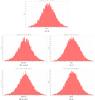 |
Fig. 6 Histogram of post-fit residuals for the astrometric parameters affected by measurement and catalog errors (see 0301 Col. in Table 1). |
4.3. Sensitivity analysis for the global PPN parameter γ
The problem in a real Gaia-like sphere reconstruction is more complex. As already mentioned above, it includes the simultaneous estimation of satellite attitude. Besides attitude, a determination of some instrument parameters is also necessary to obtain an unbiased solution. These include, for example, long-term variations of some instrument parameters, or their fine calibration to a level which cannot be reached by daily processes. The latter, however, are unrelated to the relativistic astrometric model, and are therefore out of the scope of this paper.
On the other hand, the γ parameter of the parametrized post-Newtonian formulation is indeed part of the relativistic model. It belongs to a class of unknowns of the sphere reconstruction problem which is called global because it enters in every single observation equation. In this case, the least-squares estimation cannot be reduced to the solution of N independent 5 × 5 systems of equations solving for the corrections to the catalog values of the five astrometric parameters of each of the N stars. Since the normal matrix is now block diagonal with 1-column border, it must be solved using a more complex algorithm. It has been shown (see, e.g., Bombrun et al. 2010) that the problem can be tackled by first solving the reduced normal equations for the δγ unknown, and then forwarding that solution into the N diagonal blocks to solve for the astrometric parameters. Since for each simulated sphere solution we only have one estimate of gamma, we can study its statistical properties by using a Monte-Carlo (MC) simulation.
We performed a MC experiment by running 100 simulations for the simultaneous solution of both PPN-γ and the five astrometric parameters. For this experiment the stellar sample (and the corresponding ensemble of satellite simulated observations) extracted from RDS-7-F had to be set to 12 000 primary sources because of limited resources allocated by the GSR2 system to the development (and test) infrastructure. Every MC solution provides an estimation γe of the PPN parameter1, which can be considered a random extraction from the Gaussian sample of γ estimations. The statistical accuracy in the determination of this parameter is thus given by the standard deviation of the distribution of the residuals with respect to the true value γt (=1, the GR value), namely of the variate Δγ = γt−γe.
The catalog errors for all runs were set:
-
for the astrometric quantities, to the same values as for the 0301test in Sect. 4.2;
-
for the PPN-γ, to 10-3.
Following the analysis presented in Vecchiato et al. (2003), it is possible to give an order-of-magnitude estimation of the expected accuracy on a single γ measurement by applying error propagation to the formula of gravitational light deflection (e.g., Misner et al. 1973).
In the case of a Gaussian measurement error of 125 μas, as in our simulations, and a most favorable observational configuration at 45° from the Sun, the propagated error on γ is σγ ≃ 2.5 × 10⁻². Assuming that each observation only contributes to the estimation of γ, and considering that the 12 000 primaries are observed more than 8 × 10⁶ times in 5 yr, the improvement factor of 2.8 × 10³ yields a best-accuracy value of σγ ≃ 1 × 10⁻⁵. The outcome of the MC simulation is a distribution of residuals Δγ = γt−γe centered at −6.1 × 10⁻⁵ and with a standard deviation σγMC = 1.05 × 10⁻⁴.
Despite the apparent order-of-magnitude discrepancy with the estimated accuracy above, it can be shown that this result is in fair agreement with actual expectations. Indeed, it is well known that the γ parameter is highly correlated with parallax, which is also estimated in our sphere reconstructions. For Gaia such correlation is similar to that of Hipparcos, namely ρ ≃ −0.92 (Vecchiato et al. 2003). This means that the above prediction for σγ should be increased by a factor (1−ρ2)− 1 / 2 ≃ 2.6, giving a revised value of σγ ≃ 2.6 × 10⁻⁵, that is, a factor of three better than σγMC.
We note, however, that the previous analysis does not take into account the apportionment of the measurement error between γ and the other stellar parameters. Moreover, the straightforward error propagation on the light deflection formula is based on a best-case scenario that neglects other sources of errors like, for example, a non-linear effect on the γ relative error due to the angular measurement. For these reasons, the factor of three discrepancy above appears quite reasonable.
Finally, following again the findings in (Vecchiato et al. 2003), we can extrapolate the previous value for σγMC to the case of a realistic number of observed stars. At Gaia magnitude G = 142 the number of primary stars is expected in the order of millions; if we then apply their improvement factor for the case of 1 × 10⁶G = 14 stars we get σγMC = 1.05 × 10⁻⁴/ 80 ≃ 1.3 × 10⁻⁶, a value that compares well with more recent re-estimations of the Gaia potential for the measurement of PPN-γ (Mignard & Klioner 2010; de Bruijne 2012).
5. Conclusions and perspectives
In this paper we present the latest developments of GSR-TTF, an implementation of the TTF relativistic model within the current version of the Global Sphere Reconstruction software infrastructure for the reduction of Gaia astrometric observations (GSR2) running at the DPAC DPCT. Specifically, we provide the first results of GSR-TTF as applied to five years of DPAC simulated observations.
Light propagation modeling in GSR-TTF is based on the fully relativistic (post-Minkowskian) background of the TTF. This means it can be easily expanded to take into account smaller relativistic effects on light propagation if a higher accuracy is necessary. For instance, the impact of moving axisymmetric bodies could be easily implemented by adding their formulation as given, for example, in Hees et al. (2014a).
We first provide analytical equations for both relativistic light propagation and aberration due to Gaia attitude and motion. Then, we show that GSR-TTF results for the direction cosines, that is, the observed direction, of a set of sources are equivalent to those of the GREM implementation in GaiaTools (the model and software responsible for the processing of Gaia observations, see, e.g., Balm & GaiaTools Committee 2014; ter Linden & GaiaTools Committee 2009) at the μas level or better.
The main goal of the Gaia mission is the best ever determination of positions, parallaxes and annual proper motions of all detected stars. Hence, we tested the ability of GSR-TTF to perform such a task on ~132 000 stars by using DPAC simulated observations over 5 yr. The statistical analysis of the results proves GSR-TTF is able to recover astrometric parameters with the expected accuracy when dealing with both realistic measurement and catalog errors. The estimate of instrumental parameters as well as corrections to the Gaia nominal attitude have not been included in this study but are available as part of the GSR framework and software infrastructure and will be experimented with the upcoming versions of the GSR-TTF implementation. Next, we addressed the combined estimate of astrometric parameters with the global PPN-parameter γ via a Monte-Carlo experiment. Our results appear quite consistent with the most recent works on measuring PPN-γ via Gaia’s astrometry.
GSR-TTF is then a powerful processing tool to contribute to the Gaia final catalog, for example, as additional validation resource within the Global Sphere Reconstruction system of AVU. This has already been the case, having allowed to uncover the need of an iteration for non-linearity when solving the sphere with the lower accuracy RAMOD model (RAMOD@GSR2) currently in the operational infrastructure at DPCT.
Actually, each least-squares solution provides the adjustment δγe to the γ catalog value γcat in the sense γe = γcat + δγe.
i.e., the stellar magnitude corresponding to the level of observing error we simulated.
Acknowledgments
The authors acknowledge the financial support of UIF/UFI (French-Italian University) program, CNRS/GRAM, CNES, and of the ASI contract to INAF 2014-025-R.1.2015 (Gaia Mission – The Italian Participation in DPAC). B. Bucciarelli wishes to thank the support of the Chinese Academy of Science President’s International Fellowship initiative (PIFI) for 2017. We wish to thank our DPCT colleagues for their constant support throughout this work. We also thank DPAC-CU2 for making available the Gaia simulated data used in this paper.
References
- Abbas, U., Vecchiato, A., Bucciarelli, B., Lattanzi, M. G., & Morbidelli, R. 2011, EAS Publ. Ser., 45, 127 [CrossRef] [Google Scholar]
- Balm, P., & GaiaTools Committee. 2014, Livelink Technical Note, Gaia-C1-UG-ESAC-MTL-015-02 [Google Scholar]
- Bertone, S., Le Poncin-Lafitte, C., Crosta, M., et al. 2013, in SF2A-2013: Proceedings of the Annual meeting of the French Society of Astronomy and Astrophysics, eds. L. Cambresy, F. Martins, E. Nuss, & A. Palacios, 155 [Google Scholar]
- Bertone, S., Minazzoli, O., Crosta, M., et al. 2014, Class. Quant. Grav., 31, 015021 [NASA ADS] [CrossRef] [Google Scholar]
- Bini, D., Crosta, M. T., & de Felice, F. 2003, Class. Quant. Grav., 20, 4695 [NASA ADS] [CrossRef] [MathSciNet] [Google Scholar]
- Bombrun, A., Lindegren, L., Holl, B., & Jordan, S. 2010, A&A, 516, A77 [NASA ADS] [CrossRef] [EDP Sciences] [Google Scholar]
- Brumberg, V. A. 1991, Essential relativistic celestial mechanics (Bristol, England and New York, Adam Hilger), 271 [Google Scholar]
- Crosta, M., & Vecchiato, A. 2010, A&A, 509, A37 [NASA ADS] [CrossRef] [EDP Sciences] [Google Scholar]
- Crosta, M., Vecchiato, A., de Felice, F., & Lattanzi, M. G. 2015, Class. Quant. Grav., 32, 165008 [NASA ADS] [CrossRef] [Google Scholar]
- Crosta, M., Geralico, A., Vecchiato, A., & Lattanzi, M. 2017, Phys. Rev. D, submitted [Google Scholar]
- Crosta, M. T., & Mignard, F. 2006, Class. Quant. Grav., 23, 4853 [NASA ADS] [CrossRef] [Google Scholar]
- de Bruijne, J., Siddiqui, H., Lammers, U., et al. 2010, in IAU Symp. 261, eds. S. A. Klioner, P. K. Seidelmann, & M. H. Soffel, 331 [Google Scholar]
- de Bruijne, J. H. J. 2012, Ap&SS, 341, 31 [NASA ADS] [CrossRef] [Google Scholar]
- Gaia Collaboration (Prusti, T., et al.) 2016, A&A, 595, A1 [NASA ADS] [CrossRef] [EDP Sciences] [Google Scholar]
- Hees, A., Bertone, S., & Le Poncin-Lafitte, C. 2014a, Phys. Rev. D, 90, 084020 [NASA ADS] [CrossRef] [Google Scholar]
- Hees, A., Bertone, S., & Le Poncin-Lafitte, C. 2014b, Phys. Rev. D, 89, 064045 [NASA ADS] [CrossRef] [Google Scholar]
- Klioner, S. A. 2003, AJ, 125, 1580 [Google Scholar]
- Le Poncin-Lafitte, C., Linet, B., & Teyssandier, P. 2004, Class. Quant. Grav., 21, 4463 [NASA ADS] [CrossRef] [Google Scholar]
- Le Poncin-Lafitte, C., & Teyssandier, P. 2008, Phys. Rev. D, 77, 044029 [NASA ADS] [CrossRef] [Google Scholar]
- Lindegren, L., Lammers, U., Hobbs, D., et al. 2012, A&A, 538, A78 [NASA ADS] [CrossRef] [EDP Sciences] [Google Scholar]
- Linet, B., & Teyssandier, P. 2002, Phys. Rev. D, 66, 024045 [NASA ADS] [CrossRef] [Google Scholar]
- Linet, B., & Teyssandier, P. 2013, Class. Quant. Grav., 30, 175008 [NASA ADS] [CrossRef] [Google Scholar]
- Luri, X., Martinez, O., & Isasi, Y. 2010, Livelink Technical Note, Gaia-C2-TR-UB-XL-020-01 [Google Scholar]
- Messineo, R., Morbidelli, R., Martino, M., et al. 2012, in Software and Cyberinfrastructure for Astronomy II, Proc. SPIE, 8451, 84510E [CrossRef] [Google Scholar]
- Mignard, F., & Klioner, S. A. 2010, in Relativity in Fundamental Astronomy: Dynamics, Reference Frames, and Data Analysis, eds. S. A. Klioner, P. K. Seidelmann, & M. H. Soffel, IAU Symp., 261, 306 [Google Scholar]
- Mignard, F., Bailer-Jones, C., Bastian, U., et al. 2008, in IAU Symp. 248, eds. W. J. Jin, I. Platais, & M. A. C. Perryman, 224 [Google Scholar]
- Misner, C., Thorne, K., & Wheeler, J. 1973, Gravitation (San Francisco: W. H. Freeman) [Google Scholar]
- Perryman, M. A. C., de Boer, K. S., Gilmore, G., et al. 2001, A&A, 369, 339 [NASA ADS] [CrossRef] [EDP Sciences] [Google Scholar]
- ter Linden, M., & GaiaTools Committee. 2009, Livelink Technical Note, Gaia-C1-SP-ESAC-MTL-019-01 [Google Scholar]
- Teyssandier, P., & Le Poncin-Lafitte, C. 2008, Class. Quant. Grav., 25, 145020 [NASA ADS] [CrossRef] [Google Scholar]
- Teyssandier, P., Le Poncin-Lafitte, C., & Linet, B. 2008, in Lasers, Clocks and Drag-Free Control: Exploration of Relativistic Gravity in Space, eds. H. Dittus, C. Lammerzahl, & S. G. Turyshev, Astrophys. Space Sci. Lib., 349, 153 [Google Scholar]
- Vecchiato, A., Lattanzi, M. G., Bucciarelli, B., et al. 2003, A&A, 399, 337 [NASA ADS] [CrossRef] [EDP Sciences] [MathSciNet] [Google Scholar]
- Vecchiato, A., Abbas, U., Bandieramonte, M., et al. 2012, in SPIE Conf. Ser., 8451 [Google Scholar]
- Vecchiato, A., Gai, M., Lattanzi, M. G., et al. 2014, J. Phys. Conf. Ser., 490, 012241 [CrossRef] [Google Scholar]
- Will, C. M. 2014, Liv. Rev. Relat., 17, 4 [Google Scholar]
All Tables
Results with GSR-TTF applied to 5 yr of observations of 132 K stars homogeneously distributed on the sky (in μas and μas / yr).
Results with RAMOD@GSR2 applied to 5 yr of observations of 132 K stars homogeneously distributed on the sky (in μas and μas / yr).
All Figures
|
Fig. 1 Fundamental angles in the Gaia reference frame Eâ. The two Fields of View (FoV) directions are indicated by f+ and f− while the measured abscissa is given by n(i) = (α,β,δ) (from Vecchiato et al. 2012). |
| In the text | |
|
Fig. 2 Difference between the abscissae resulting from the GSR-TTF implementation and from GREM implementation in the “GaiaTools”. The left axis indicates the difference in μas between the two models – represented by the red plot; the right axis indicates the distance in degrees between a given planet and the observation – the blue, yellow and green plot representing Jupiter, Saturn and the Earth, respectively. |
| In the text | |
|
Fig. 3 Abscissae differences between the GSR-TTF and GREM implementations. The vast majority of the observations show differences in the interval of ± 0.2 μas, well below the accuracy required by Gaia. |
| In the text | |
|
Fig. 4 Frequency of observations as function of celestial coordinates due to Gaia scanning law (blue ≈50 – yellow ≈500). |
| In the text | |
|
Fig. 5 Astrometric post-fit residuals for a set of 132 000 stars as function of the number of observations for each star (red: ϖ, blue: αcosδ, green: δ, yellow: μαcosδ, purple: μδ) . |
| In the text | |
|
Fig. 6 Histogram of post-fit residuals for the astrometric parameters affected by measurement and catalog errors (see 0301 Col. in Table 1). |
| In the text | |
Current usage metrics show cumulative count of Article Views (full-text article views including HTML views, PDF and ePub downloads, according to the available data) and Abstracts Views on Vision4Press platform.
Data correspond to usage on the plateform after 2015. The current usage metrics is available 48-96 hours after online publication and is updated daily on week days.
Initial download of the metrics may take a while.