| Issue |
A&A
Volume 608, December 2017
|
|
|---|---|---|
| Article Number | A131 | |
| Number of page(s) | 9 | |
| Section | Astrophysical processes | |
| DOI | https://doi.org/10.1051/0004-6361/201731519 | |
| Published online | 15 December 2017 | |
The glitch activity of neutron stars
1 Instituto de Astrofísica, Pontificia Universidad Católica de Chile, Av. Vicuña Mackenna 4860, 7820436 Macul, Santiago Chile,
e-mail: This email address is being protected from spambots. You need JavaScript enabled to view it.
2 Departamento de Física, Universidad de Santiago de Chile, Avenida Ecuador 3493, 9170124 Estación Central, Santiago, Chile
3 Jodrell Bank Centre for Astrophysics, School of Physics and Astronomy, The University of Manchester, Manchester M13 9PL, UK
Received: 6 July 2017
Accepted: 3 October 2017
Abstract
We present a statistical study of the glitch population and the behaviour of the glitch activity across the known population of neutron stars. An unbiased glitch database was put together based on systematic searches of radio timing data of 898 rotation-powered pulsars obtained with the Jodrell Bank and Parkes observatories. Glitches identified in similar searches of 5 magnetars were also included. The database contains 384 glitches found in the rotation of 141 of these neutron stars. We confirm that the glitch size distribution is at least bimodal, with one sharp peak at approximately 20 μHz, which we call large glitches, and a broader distribution of smaller glitches. We also explored how the glitch activity ν̇g, defined as the mean frequency increment per unit of time due to glitches, correlates with the spin frequency ν, spin-down rate |ν̇|, and various combinations of these, such as energy loss rate, magnetic field, and spin-down age. It is found that the activity is insensitive to the magnetic field and that it correlates strongly with the energy loss rate, though magnetars deviate from the trend defined by the rotation-powered pulsars. However, we find that a constant ratio ν̇g/|ν̇| = 0.010 ± 0.001 is consistent with the behaviour of all rotation-powered pulsars and magnetars. This relation is dominated by large glitches, which occur at a rate directly proportional to |ν̇|. For low |ν̇|, only small glitches have been detected, making the inferred glitch activity formally lower than that predicted by the constant ratio, in many cases zero. However, we can attribute this to the low predicted rate for large glitches, together with the insufficient observing time, which makes it unlikely to detect any large glitches in this range. Taking this into consideration, we show that the behaviour of each rotation-powered pulsar and magnetar is statistically consistent with the above relationship, including those objects where no glitches have been detected so far. The only exception are the rotation-powered pulsars with the highest values of |ν̇|, such as the Crab pulsar and PSR B0540−69, which exhibit a much smaller glitch activity, intrinsically different from each other and from the rest of the population. The activity due to small glitches also shows an increasing trend with |ν̇|, but this relation is biased by selection effects.
Key words: stars: neutron / stars: magnetars / pulsars: general / stars: rotation
© ESO, 2017
1. Introduction
Rotation-powered pulsars (hereafter just “pulsars”) and magnetars are believed to be highly magnetized, rotating neutron stars. Their spin can be tracked with high accuracy over years using standard timing techniques (Ryba & Taylor 1991a,b; Kaspi et al. 1994). Their rotation is generally stable and shows a regular spin-down trend (frequency derivative  ). Nevertheless, many pulsars exhibit sudden increases in their rotation frequency ν, known as glitches. Glitches have relative sizes Δν/ν ~ 10-11−10-5, and in most cases, are followed by an increase in the spin-down rate
  of the star, with relative magnitudes
  . Several mechanisms have been suggested to explain these phenomena (see, for instance, Haskell & Melatos 2015, for a recent review of glitch models). The lack of observed radiative changes associated with these events in nearly all rotation-powered pulsars suggests an internal origin. In this context, glitches are believed to be caused by a rapid transfer of angular momentum from a neutron superfluid in the inner crust to the rest of the star (Anderson & Itoh 1975; Alpar et al. 1984). However, glitches in magnetars (and also in the high magnetic field pulsars J1119−6127 and J1846−0258) are sometimes accompanied by radiative changes, and could have a different origin (Dib & Kaspi 2014; Kaspi & Beloborodov 2017).
Observations of glitches represent one of the very few instances through which we can indirectly inspect the interior of a neutron star. For example, attempts have been made to use glitches to put constraints on the structural properties of neutron stars, their masses, and the equation of state of dense matter (Link et al. 1999; Chamel 2012, 2013; Ho et al. 2015; Pizzochero et al. 2017). Recent studies of the rotation of young neutron stars, such as the Vela and Crab pulsars, suggest that the effects of glitches over the long-term spin evolution are comparable to the effects driven by magnetic braking or stellar winds (Lyne et al. 1996, 2015; Espinoza et al. 2017).
Trends in the glitch behavior of pulsars have been slowly emerging as the number of detected glitches increases. McKenna & Lyne (1990) and Lyne et al. (2000) showed that the glitch activity describes a linear behavior with the spin-down rate  of the star. Espinoza et al. (2011), using a larger sample, confirmed this result and found that the glitch activity decreases rapidly in pulsars with low spin-down rate. They also established that young pulsars exhibit glitches more often than old pulsars, and found that the size distribution of all observed glitches has a bimodal appearance. Furthermore, they found that most of the largest glitches are produced by a small group of relatively young pulsars, suggesting that the bimodality of the glitch size distribution could be produced by two different classes of pulsars or by a glitch mechanism that evolves as pulsars age.
This work is intended to be an extension of the previous study by Espinoza et al. (2011). It presents the building and analysis of a sample of glitches that is unbiased towards their presence in the data. The events were taken from published systematic records of timing observations of hundreds of pulsars. We focus on the frequency step sizes and their rate (the glitch activity) and study how they depend on long-term spin properties (spin frequency, spin-down rate, and combinations of these, such as energy-loss rate, magnetic field, and spin-down age). This paper is organised as follows. Section 2 describes the new database and how neutron stars and glitch detections were selected to avoid bias in our sample. In Sect. 3 we analyze the glitch size distribution and classify glitches according to their sizes. Section 4 presents a study of the cumulative effect of glitches on the rotation of neutron stars and a discussion of the relation between the glitch activity and the spin-down rate. Finally, Sects. 5 and 6 show the Discussions and Conclusions of the paper, respectively.
2. The new database
Today, more than 700 pulsars are regularly monitored at the Jodrell Bank Observatory (JBO), some of them from as early as 1978 (Hobbs et al. 2004). These long-term observations are essential to finding glitches and studying their properties. In order to build a sample that is as unbiased as possible, we included all pulsars that have been regularly monitored for glitches in clearly defined time spans, regardless of whether glitches were found or not. Selecting only those pulsars for which glitches have been detected would bias the sample towards the presence of glitches. According to this scheme, we included 778 pulsars monitored at JBO, containing 296 glitches in the rotation of 111 pulsars. These glitches are the JBO events in Espinoza et al. (2011) plus 69 newer glitches measured until 2015 and published in the JBO online glitch catalog 1 (Shaw et al., in prep.).
In order to expand the sample, we also included Parkes observations of 118 pulsars, which show 73 glitches in the rotation of 23 pulsars, as reported by Yu et al. (2013). In case of overlap between the observation spans of the JBO and Parkes pulsars, we considered the earliest and the latest epoch between the two to define the start and end of the searched time spans.
In order to improve the statistics for pulsars with small characteristic ages ( ), we also added the two X-ray pulsars PSRs J1846-0258 and B0540-69, which have been monitored for about 15 yr each and have been searched for glitches (Ferdman et al. 2015; Livingstone et al. 2011). With these two additions, the database contains all the rotation-powered pulsars known with τc< 2 kyr. It is not possible to obtain a complete sample for pulsars of larger characteristic ages because many of them have either not been regularly monitored or not been searched for glitches.
Finally, to compare the glitch activity between rotation-powered pulsars and magnetars, we included the observations of five magnetars. They have been observed continuously for 16 yr on average, and Dib & Kaspi (2014) reported a set of 11 glitches in the whole of their timing dataset.
We constructed a database containing rotational information (ν, ), with corrected for the Shklovskii effect (Camilo et al. 1994), glitch measurements Δν, and the observation spans over which glitch searches have been performed (on average, 17.5 yr for each pulsar). Here, Δν corresponds to the frequency increase due to the glitch. We did not take  steps or recoveries into account because not all glitches have these parameters measured in a consistent way.
Altogether, our sample contains the rotational information of 903 neutron stars, as shown in Fig. 1, with a total of 384 glitches in 141 of them. The sample does not have a well-defined selection criteria, being mostly determined by having pulsars bright enough that they could be regularly monitored without an extreme commitment of observing time. In addition, the observing time spans are not uniform, as additional pulsars were added as they were discovered. On the other hand, it is important to note that the sample includes nearly a third of all pulsars known to date, with representatives across the P−Ṗ diagram (see Fig. 1), and none of the pulsars were selected directly because of their glitch properties (presence or absence of glitches, their frequency, or size). Thus, it should be close to the best possible available sample for the study performed in the present paper, and the biases present should not affect our conclusions.
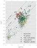 |
Fig. 1 Rotation period versus its time derivative (“P-Ṗ diagram”) for all known neutron stars. Lines of constant spin-down rate |
3. The glitch size distribution
The distribution of the glitch magnitude Δν of all glitches in our database is shown in Fig. 2, and is in agreement with the bimodal shape reported by Espinoza et al. (2011) and Ashton et al. (2017). There is a broad distribution of small glitches and a very narrow distribution of large glitches which peaks around 20 μHz. It is worth mentioning that this peak contains 70 large glitches detected in 38 different pulsars, where the main contributor is PSR J1420−6048, with 5 large glitches. This confirms that this peak of large glitches is by no means the effect of only a handful of pulsars.
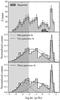 |
Fig. 2 Histogram of the glitch size Δν of all glitches in our database. In the upper panel the error bars correspond to the square root of the number of events per bin. The middle and lower panels show the best fits with one, two, and three Gaussians. Magnetar glitches were not included in the latter panels nor in the fits. The solid and dashed lines represent the best fits and their components, respectively. The shaded region indicates that glitches of sizes smaller than 0.01μHz may be missing due to detectability issues. |
As noted by Espinoza et al. (2011), the left edge of the distribution is unconstrained since detections of very small glitches are strongly limited by the cadence of the observations, their sensitivity, and the intrinsic rotational noise of the pulsar. Given that these properties vary from pulsar to pulsar, it is not straightforward to set a universal lower detectability limit for the glitch size distribution of all pulsars (Fig. 2). However, based on the comparison of glitch sizes obtained by different authors, Espinoza et al. (2011) argued that for sizes below Δν/ν ~ 10-8 the sample is likely to start being incomplete. Using the detectability limits for individual sources proposed by Espinoza et al. (2014), it is possible to calculate average detection limits for all glitches. For an observing cadence of 30 days and a rotational noise (or minimum sensitivity) of 0.01 rotational phases, glitch detection is severely compromised below sizes Δν ~ 10-2μHz. This is consistent with the Δν/ν figure quoted above (for young pulsars). Hence glitches with magnitudes below this limit are likely to be missed, especially if their frequency derivative steps are larger than  (see Watts et al. 2015). This is a conservative limit because many pulsars are observed more frequently and exhibit lower noise levels.
In the following, we model the glitch size distribution as a sum of Gaussian distributions. We note, however, that the detection issues discussed above must be considered when using such functions to describe the population of small glitches. Models composed of one and up to four Gaussians were tested against the data. The best fits obtained are shown in Fig. 2 (middle and lower panels; see Table A.1 for the parameters of the fits). Using Akaike’s information criterion (hereafter AIC, see Appendix A for a brief description of the test and the results obtained), we conclude that among the whole set of candidate models, a mixture of three Gaussians gives the best description of the glitch size distribution. All fits performed with more than one Gaussian give a common component (with nearly identical parameters) that contains all the glitches with magnitudes Δν ≥ 10 μ Hz. Because of this and the multimodal nature of the distribution, we classify glitches as large and small using Δν = 10 μHz as the dividing line. We also made fits for the Δν/ν distribution, and the AIC suggests, as for Δν, a non-unimodal behavior, although with two broader peaks of similar height. This further supports the multimodal interpretation of the glitch size distribution.
4. Glitch activity
A practical way to quantify the cumulative effects of a collection of spin-ups due to glitches on a pulsar’s rotation is through the glitch activity. This parameter is defined as the time-averaged change of the rotation frequency due to glitches. Due to the short length of the observation spans available, it is not possible to detect enough glitches for a robust estimation for each pulsar. To avoid this problem, we studied the combined glitch activity for groups of pulsars sharing a common property. Following Lyne et al. (2000) and Espinoza et al. (2011), the average glitch activity for each group is 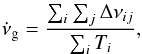 (1)where the double sum runs over every change in frequency Δνij due to the glitch j of the pulsar i, and Ti is the time over which pulsar i has been searched for glitches. This analysis includes those pulsars that have been searched, but not found to glitch so far. Since the errors in the measurements of the glitch sizes are smaller than the Poisson fluctuations in the number of glitches detected due to finite observation spans, the errors for
  are estimated as
 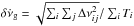 (for more details see Appendix B). Unlike those presented in Lyne et al. (2000) and Espinoza et al. (2011), these errors account for the presence of glitches of different sizes. However, our formula still does not take into account the possible contribution of rare, large glitches that were not detected because of the finite monitoring times. This implies that the error bars for
  are likely underestimated.
4.1. Dependence on spin parameters
We grouped the pulsars in bins of width equal to 0.5 in logarithmic scale according to different properties (spin frequency ν, spin-down rate , and various combinations of these, such as energy-loss rate  , magnetic field
  , and spin-down age
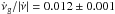
  ). Figure 3 shows how depends on these variables. Considering only rotation-powered pulsars, we observe that , Ėrot, and τc appear to give good correlations, whereas there are no clear correlations with B and ν.
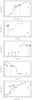 |
Fig. 3 Glitch activity as a function of various pulsar parameters (all of them combinations of frequency ν and its time-derivative |

It is also apparent in Fig. 3 that the glitch activity of the magnetars with the smallest characteristic ages is lower than that of the rotation-powered pulsars with similar characteristic ages. However, their activity is larger than that of pulsars of equal spin-down power. The only parameter for which the glitch activity of magnetars appears to follow the same relation as for rotation-powered pulsars is the spin-down rate. Because there is almost no overlap between the spin frequencies and magnetic fields of magnetars, and those of the rotation-powered pulsars, the comparison is not possible for these parameters. Interestingly, however, it seems that the glitch activity of pulsars and magnetars does not appear to depend directly on their dipolar magnetic field strength. On the other hand, in the case of magnetars, some glitches are contemporaneous with X-ray bursts, which are thought to be powered by the decay of their strong magnetic fields (Dib & Kaspi 2014; Kaspi & Beloborodov 2017). Similarly, the largest glitches in the high magnetic field pulsars PSRs J1119−6127 and J1846−0258 were accompanied by changes in their emission properties (Livingstone et al. 2010; Weltevrede et al. 2011; Archibald et al. 2016). This possible connection between glitches and magnetospheric processes has lead to the idea that some glitches in high magnetic field neutron stars could have a different origin. Our results show, however, that the spin-down rate might be what determines the rate and size of these glitches, just as it does for ordinary pulsars.
We choose as the best parameter to study , because we can interpret our results in terms of simple physical concepts, and because this is the only parameter for which magnetars follow a similar tendency to rotation-powered pulsars. It is worth mentioning that we tested a broad range of combinations of the form  with different values of a, finding that none of them give a substantially better correlation with than
  .
.
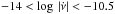
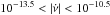
Figure 4 confirms the relation  already reported by Lyne et al. (2000) and Espinoza et al. (2011) for pulsars with
  (we always take the units of as Hzs-1). The mean value of the ratio
  for this range is 0.012 ± 0.001, corresponding to the horizontal line in Fig. 4b. This represents the fraction of the spin-down “recovered” by glitches, which can be interpreted as the fraction of the star’s moment of inertia in a decoupled internal component (Link et al. 1999). However, the linear trend between the glitch activity and the spin-down rate seems to fail towards the extremes, which we will explore further in Sect. 4.2. Table 1 shows additional information related to each bin in Fig. 4.
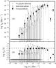 |
Fig. 4 Panel a: |


4.2. A common trend in the activity of nearly all pulsars
Motivated by the results in Sect. 3 showing that the largest glitches separate from the rest, we re-computed the glitch activity separately for large glitches (Δν ≥ 10 μHz) and for small glitches (the remainder), showing the results in Fig. 5. We observe that large glitches determine the linear relation between and in the range  , and calculate the ratio
 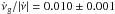 . This value is consistent with the value obtained in the previous section, when considering all glitches and including bin 7, which has no large glitches detected. Accordingly, we use the linear relation
  as a reference throughout the paper. The activity due to small glitches follows a roughly similar, though noisier, increasing trend with .
Statistics of glitches for pulsars binned by their spin-down rate.
There are no large glitches detected in pulsars with the smallest and the largest spin-down rates ( and
and  ). The 14th bin (
 , Table 1) fails to follow the linear trend, despite having four large glitches with average size of 37 μHz. For the accumulated observing time in this bin, approximately 30 additional large glitches of 20 μHz are required to reach the activity value predicted by the linear relation. On the other side, the 7th bin (
 ) follows the linear trend even though it has no large glitches detected. According to the linear relation and the accumulated observing time, only one large glitch of 10 μHz is necessary to obtain the value predicted by the linear trend, which is very close to the current activity value. However, instead of one large glitch, there are smaller glitches that account for 9.78 μHz, making the activity consistent with the linear relationship.
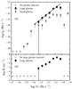 |
Fig. 5 Panel a: |

Since the proportionality between the glitch activity and the spin-down rate is dominated by large glitches, and these have a very narrow size distribution, we expect that the rate of large glitches, Ṅℓ, will also be proportional to (Fig. 5b). Because the number of large glitches is expected to follow a Poisson distribution, the expected dispersion in the rate of large glitches Ṅℓ can be estimated in a more reliable way than that in the glitch activity . This allows us to test in a statistically meaningful way whether or not the identified trend applies to all pulsars.
Figure 6 confirms that  is approximately constant and its mean value is (4.2 ± 0.5) × 102Hz-1 (which we calculated considering only the bins for pulsars with
  ). We observe that except for the three bins with the largest spin-down rate, all others are consistent with this trend. The non-detection of large glitches in the region of small is consistent with the small expected rate and the finite monitoring time, as illustrated by the shaded area in Fig. 6. Based on this relation, the expected number of large glitches (
 ) for the three bins with the highest (
 ) is 30 ± 5, 35 ± 5, and 325 ± 18, respectively. This strongly contradicts the only four large glitches detected in bin 14 and the absence of large glitches in bins 15 and 16 (which contain only PSR B0540−69 and the Crab pulsar, respectively; see Table 1). Thus, we can confidently rule out the linear relation between and for the largest values of the latter variable, but it remains consistent for all
  Hz s-1.
 |
Fig. 6
|


Next, we test whether the individual pulsars within each bin are also consistent with this trend. Since the number of large glitches for each pulsar is small (in most cases zero), the usual χ2 test is not applicable. Instead, we use Fisher’s test (Fisher 1925), based on the statistic  (2)with two-tailed p-values for each pulsar calculated as
  (3)where
  is the (Poisson) probability of observing a value
  smaller or equal to the expected value , based on the fixed ratio
  calculated above (and analogously for
 ![Mathematical equation: \hbox{$P[N^{\rm{obs}}_{\rm{\ell}} \geq N^{\rm{exp}}_{\rm{\ell}}])$}](/articles/aa/full_html/2017/12/aa31519-17/aa31519-17-eq117.png) .
.
If the null hypothesis is true, pi is uniformly distributed between 0 and 1, and therefore the Fisher statistic will follow a χ2 distribution with 2k degrees of freedom. On the other hand, when the individual p-values pi are very small,  will be large, leading to the rejection of the global null hypothesis.
Table 2 shows the results of the test, where the global p-value for each bin was calculated as  (4)that is, the probability of obtaining a χ2 value at least as large as our observed
  , under the null hypothesis
  . Based on the values obtained for pbin, the null hypothesis can be strongly ruled out for the last three bins, whereas we cannot rule out that all pulsars with Hz s-1, even those without glitches, follow the identified trend.
Results of Fisher’s method.
5. Discussion
We have shown that all pulsars with  and magnetars are consistent with a single trend, dominated by large glitches, in which the glitch activity is equal to
  . The large collection of pulsars with no detected glitches is also consistent with this trend. For instance, the predicted rate of large glitches for pulsars with
  (bin 6) is one large glitch every ~ 104 yr, whereas the accumulated observing time in this bin is only 1973 yr (Table 1), and this mismatch becomes even more extreme for the bins with lower . This means that there are no reasons to reject the idea that every neutron star will eventually experience a large glitch and will, in the long-term, follow the above relationship. On the other hand, we cannot rule out the possibility that, for example, the glitch mechanism could fail to produce large glitches in the pulsars with the smallest spin-down rates, or produce substantially more of them than predicted from the linear relation.
A similar amount of superfluid neutrons inside all neutron stars could be responsible for the common glitch activity levels observed (Link et al. 1999). However, despite this uniformity in the collective behavior, it appears that the glitch mechanism possesses an intrinsic bi-modality (Fig. 2). It could be that the mechanism results in different glitch sizes and rates depending on where in the star the glitch happens (Haskell et al. 2012; Haskell & Antonopoulou 2014). An alternative interpretation is that there are two or more different glitch mechanisms in action, giving rise to different size distributions.
The cumulative distributions of glitch sizes for five individual pulsars, presented in Fig. 16 of Espinoza et al. (2011), suggests that this bi-modality could be extended to define at least two types of pulsars: those with large glitches and those with only small glitches; but we find no evidence for this in the glitch activity data.
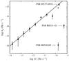 |
Fig. 7 A zoom-in to the zone |

5.1. The glitch behavior of the most rapidly evolving pulsars
The glitch activity for the last two bins was calculated using only one pulsar per bin (see Table 1) and the values obtained do not follow the tendency defined by the rest of the population. These are the pulsars with the largest spin-down rates and correspond to PSR B0540−69 (bin 15) and the Crab pulsar (PSR B0531+21, bin 16). PSR B0540−69 has been observed for ~ 15.8yr (Ferdman et al. 2015) and its activity is especially low, compared to all pulsars with high spin-down rates (see Fig. 4). In the same bin it is possible to include the X-ray pulsar PSR J0537−6910, which was not considered in our sample since it does not belong to any of the monitoring programs taken into account for our database, and including it would have artificially biased the sample towards the presence of glitches. It has been observed for 13yr, and 45 glitches have been detected (Marshall et al. 2004; Middleditch et al. 2006; Antonopoulou et al. 2017; Ferdman et al. 2017), 30 of which are large according to our classification in Sect. 3, making it consistent with the linear trend identified above. If we included this pulsar in our dataset, the glitch activity in the associated bin would be only slightly lower than predicted by the relation  (see Fig. 7).
Marshall et al. (2015) reported a large increase in the spin-down rate of PSR B0540−69 that remained for < 3 yr. Based on their data, they placed a limit of Δν< 12μHz for a hypothetical glitch responsible for this increase. With a glitch of the maximum allowed size, the activity of PSR B0540−69 would be 2(2) × 10-14Hzs-1, very similar to the activity of the Crab pulsar 1.1(5) × 10-14Hzs-1, but still low if the pulsar was to follow the relationship above.
One possible explanation for the discrepancy in the glitch activity of these pulsars could be their age, as proposed by Alpar et al. (1996) to explain the differences between the Crab and Vela pulsars. Indeed, PSR B0540−69 and the Crab pulsar are among the youngest pulsars known, with supernova remnant ages equal to  and 962 yr, respectively (Park et al. 2010; Ho & Andersson 2012). However, other similarly young pulsars, such as PSRs J1119−6127 and J1846−0258 (in bins 13 and 14, respectively), but with lower spin-down rates, have experienced large glitches during their monitored rotations and exhibit glitch activities in closer agreement with the main trend. We conclude that it is possible that the glitch mechanism might not be able to operate normally when the spin-down rate is too high. Perhaps, once PSR B0540−69 and the Crab pulsar have evolved, and their spin-down rates have decreased, their glitches will have settled into the trend followed by the rest of the population.
6. Conclusions
In this paper we present a statistical study of glitches in pulsars and magnetars, using a large database of pulsars whose selection was independent of their glitch properties. The main conclusions are the following:
-
1)
The glitch size distribution is at least bimodal, with twowell-defined classes: a broad distribution of small glitches and anarrow one with large glitches peaked at around20 μHz. However, there is no evidence in the glitch activity data for the existence of two classes of pulsars.
-
2)
For pulsars and magnetars with
 Hz s-1, the glitch activity is directly proportional to the spin-down rate , following
 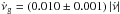 . This relationship is dominated by large glitches. For all pulsars in this group, the rate of large glitches is consistent with the proportionality relation
 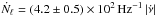 . This is also consistent for the pulsars with
  , which have not been observed long enough to detect large glitches. Thus, we showed that the glitch activity of every pulsar with , including those with no glitches, is statistically consistent with the above relationships.
 -
3)
The activity due to small glitches also increases with
. We did not present an explicit relation between the activity of small glitches and because it depends strongly on the choice of the cutoff value between small and large glitches, and on detectability issues. -
4)
Pulsars with
 Hz s-1 present an intrinsically different behavior, with a much lower rate of large glitches.
Future studies, based on the analysis of glitches in individual pulsars, should provide information helping clarify whether there are two or more glitch mechanisms giving rise to the observed multimodal glitch size distribution. For this, well designed, long-term monitoring campaigns are needed, in which cadence and sensitivity are combined to ensure the detection of small glitches, thereby improving the completeness of the current samples.
Acknowledgments
We thank Danai Antonopoulou for useful comments. This work was funded by ALMA-CONICYT Astronomy/PCI Project 31140029, FONDECYT Regular Projects 1150411 and 1171421, CONICYT Basal Funding Grant PFB-06, CONICYT grant PIA ACT1405, and a SOCHIAS travel grant through ALMA/Conicyt Project #31150039. We thank the observers at Jodrell Bank Observatory. Pulsar research at Jodrell Bank Centre for Astrophysics (JBCA) is supported by a consolidated grant from the UK Science and Technology Facilities Council (STFC).
References
- Akaike, H. 1974, IEEE Transactions on Automatic Control, 19, 716 [Google Scholar]
- Alpar, M. A., Pines, D., Anderson, P. W., & Shaham, J. 1984, ApJ, 276, 325 [NASA ADS] [CrossRef] [Google Scholar]
- Alpar, M. A., Chau, H. F., Cheng, K. S., & Pines, D. 1996, ApJ, 459, 706 [NASA ADS] [CrossRef] [Google Scholar]
- Anderson, P. W., & Itoh, N. 1975, Nature, 256, 25 [NASA ADS] [CrossRef] [Google Scholar]
- Antonopoulou, D., Espinoza, C. M., Kuiper, L., & Andersson, N. 2017, MNRAS, 473, 1644 [Google Scholar]
- Archibald, R. F., Kaspi, V. M., Tendulkar, S. P., & Scholz, P. 2016, ApJ, 829, L21 [NASA ADS] [CrossRef] [Google Scholar]
- Ashton, G., Prix, R., & Jones, D. I. 2017, Phys. Rev. D, 96, 063004 [NASA ADS] [CrossRef] [Google Scholar]
- Camilo, F., Thorsett, S. E., & Kulkarni, S. R. 1994, ApJ, 421, L15 [NASA ADS] [CrossRef] [Google Scholar]
- Chamel, N. 2012, Phys. Rev. C, 85, 035801 [NASA ADS] [CrossRef] [Google Scholar]
- Chamel, N. 2013, Phys. Rev. Lett., 110, 011101 [NASA ADS] [CrossRef] [PubMed] [Google Scholar]
- Dib, R., & Kaspi, V. M. 2014, ApJ, 784, 37 [NASA ADS] [CrossRef] [Google Scholar]
- Espinoza, C. M., Lyne, A. G., Stappers, B. W., & Kramer, M. 2011, MNRAS, 414, 1679 [NASA ADS] [CrossRef] [Google Scholar]
- Espinoza, C. M., Antonopoulou, D., Stappers, B. W., Watts, A., & Lyne, A. G. 2014, MNRAS, 440, 2755 [NASA ADS] [CrossRef] [Google Scholar]
- Espinoza, C. M., Lyne, A. G., & Stappers, B. W. 2017, MNRAS, 466, 147 [NASA ADS] [CrossRef] [Google Scholar]
- Ferdman, R. D., Archibald, R. F., & Kaspi, V. M. 2015, ApJ, 812, 95 [NASA ADS] [CrossRef] [Google Scholar]
- Ferdman, R. D., Archibald, R. F., Gourgouliatos, K. N., & Kaspi, V. M. 2017, ApJ, submitted [arXiv:1708.08876] [Google Scholar]
- Fisher, R. 1925, Statistical Methods For Research Workers, Cosmo study guides (Cosmo Publications) [Google Scholar]
- Haskell, B., & Antonopoulou, D. 2014, MNRAS, 438, L16 [NASA ADS] [CrossRef] [Google Scholar]
- Haskell, B., & Melatos, A. 2015, Int. J. Mod. Phys. D, 24, 1530008 [NASA ADS] [CrossRef] [Google Scholar]
- Haskell, B., Pizzochero, P. M., & Sidery, T. 2012, MNRAS, 420, 658 [NASA ADS] [CrossRef] [Google Scholar]
- Ho, W. C. G., & Andersson, N. 2012, Nat. Phys., 8, 787 [NASA ADS] [CrossRef] [Google Scholar]
- Ho, W. C. G., Espinoza, C. M., Antonopoulou, D., & Andersson, N. 2015, Sci. Adv., 1, e1500578 [NASA ADS] [CrossRef] [Google Scholar]
- Hobbs, G., Lyne, A. G., Kramer, M., Martin, C. E., & Jordan, C. 2004, MNRAS, 353, 1311 [NASA ADS] [CrossRef] [Google Scholar]
- Ivezic, Z., Connolly, A. J., VanderPlas, J. T., & Gray, A. 2014, Statistics, Data Mining, and Machine Learning in Astronomy: A Practical Python Guide for the Analysis of Survey Data (Princeton: Princeton University Press) [Google Scholar]
- Kaspi, V. M., & Beloborodov, A. M. 2017, ARA&A, 55, 261 [NASA ADS] [CrossRef] [Google Scholar]
- Kaspi, V. M., Taylor, J. H., & Ryba, M. F. 1994, ApJ, 428, 713 [NASA ADS] [CrossRef] [Google Scholar]
- Link, B., Epstein, R. I., & Lattimer, J. M. 1999, Phys. Rev. Lett., 83, 3362 [NASA ADS] [CrossRef] [Google Scholar]
- Livingstone, M. A., Kaspi, V. M., & Gavriil, F. P. 2010, ApJ, 710, 1710 [NASA ADS] [CrossRef] [Google Scholar]
- Livingstone, M. A., Ng, C.-Y., Kaspi, V. M., Gavriil, F. P., & Gotthelf, E. V. 2011, ApJ, 730, 66 [NASA ADS] [CrossRef] [Google Scholar]
- Lyne, A. G., Pritchard, R. S., Graham-Smith, F., & Camilo, F. 1996, Nature, 381, 497 [NASA ADS] [CrossRef] [Google Scholar]
- Lyne, A. G., Shemar, S. L., & Smith, F. G. 2000, MNRAS, 315, 534 [NASA ADS] [CrossRef] [Google Scholar]
- Lyne, A. G., Jordan, C. A., Graham-Smith, F., et al. 2015, MNRAS, 446, 857 [NASA ADS] [CrossRef] [Google Scholar]
- Manchester, R. N., Hobbs, G. B., Teoh, A., & Hobbs, M. 2005, AJ, 129, 1993 [NASA ADS] [CrossRef] [Google Scholar]
- Marshall, F. E., Gotthelf, E. V., Middleditch, J., Wang, Q. D., & Zhang, W. 2004, ApJ, 603, 682 [NASA ADS] [CrossRef] [Google Scholar]
- Marshall, F. E., Guillemot, L., Harding, A. K., Martin, P., & Smith, D. A. 2015, ApJ, 807, L27 [NASA ADS] [CrossRef] [Google Scholar]
- McKenna, J., & Lyne, A. G. 1990, Nature, 343, 349 [NASA ADS] [CrossRef] [Google Scholar]
- Middleditch, J., Marshall, F. E., Wang, Q. D., Gotthelf, E. V., & Zhang, W. 2006, ApJ, 652, 1531 [NASA ADS] [CrossRef] [Google Scholar]
- Park, S., Hughes, J. P., Slane, P. O., Mori, K., & Burrows, D. N. 2010, ApJ, 710, 948 [NASA ADS] [CrossRef] [Google Scholar]
- Pizzochero, P. M., Antonelli, M., Haskell, B., & Seveso, S. 2017, Nat. Astron., 1, 0134 [NASA ADS] [CrossRef] [Google Scholar]
- Ryba, M. F., & Taylor, J. H. 1991a, ApJ, 371, 739 [NASA ADS] [CrossRef] [Google Scholar]
- Ryba, M. F., & Taylor, J. H. 1991b, ApJ, 380, 557 [NASA ADS] [CrossRef] [Google Scholar]
- Watts, A., Espinoza, C. M., Xu, R., et al. 2015, Advancing Astrophysics with the Square Kilometre Array (AASKA14), 43 [Google Scholar]
- Weltevrede, P., Johnston, S., & Espinoza, C. M. 2011, MNRAS, 411, 1917 [NASA ADS] [CrossRef] [Google Scholar]
- Yu, M., Manchester, R. N., Hobbs, G., et al. 2013, MNRAS, 429, 688 [NASA ADS] [CrossRef] [Google Scholar]
Appendix A: Model selection: Akaike’s information criterion applied to the glitch size distribution
Given a model M that includes k parameters θp, p = 1,...,k, abbreviated as the vector θ with components θp, we can compute the likelihood p(xi | θ) of observing any given datum xi. If we assume that our data { xi } are all independent of each other, the likelihood of the whole dataset is given by  (A.1)Once the likelihood for a set of models is known, the model with the largest value provides the best description of the dataset. However, this is not necessarily the best model overall when models have different numbers of free parameters. Akaike’s information criterion (AIC) is defined as
  (A.2)(Akaike 1974), where L is the likelihood of the dataset given the model, and k is the number of free parameters of the model. According to the AIC, the best model is the one with the smallest AIC value. The AIC penalizes for the addition of parameters, and therefore selects a model that fits well and has a minimum number of parameters. We note that the AIC value by itself has no meaning, and only has significance when compared to the values for a set of alternative models.
In order to compare the models, we need two measures: the relative AIC and Akaike weights. The relative AIC is the difference of a given candidate model m in respect to the model with the minimum AIC value  (A.3)where (AIC)m is the AIC value for the model m, and (AIC)min is the AIC value of the best candidate model. Akaike weights wm represent the probability that the model m is the best model (in the AIC sense, that it minimizes the loss of information), given the data and the whole set of candidate models:
  (A.4)so that ∑ mwm = 1.
In order to test if the glitch size distribution is multimodal, we modeled it as a sum of M Gaussians, writing the likelihood of a datum xi = log Δνi as  (A.5)where θ denotes the vector of parameters that need to be estimated; it includes normalization factors for each Gaussian, αj (with the constraint that ∑ jαj = 1), and its mean μj and dispersion σj. Using the Expectation-Maximization algorithm described in Ivezic et al. (2014), we obtained the parameters that maximize the log-likelihood of the whole dataset { xi }, for models with one, two, three, and four Gaussians. In order to decide the model that gives the best description of the data, we applied the AIC and calculated the Akaike weights wm for each model according to Eq. (A.4). Table A.1 summarizes the results.
Results of the expectation-maximization algorithm and the AIC applied to the glitch size distribution modeled as a sum of Gaussians.
The Akaike weight associated to the model with three components is w3 = 0.957, that is, it has a 95.7 % probability of being the best one among the candidate models considered.
Appendix B: Error estimation of the glitch activity
In order to estimate the error in , we assume that detections of glitches of any given size follow Poisson statistics. If we detected N glitches with a magnitude equal to Δν, in an observation span T, we can write the glitch activity as  (B.1)and its variance as
 ![Mathematical equation: \appendix \setcounter{section}{2} \begin{equation} \text{Var}\left[\dot{\nu}_{\rm{g}}\right] = \left(\dfrac{\Delta \nu}{T}\right)^2\text{Var}\left[N\right] = \left(\dfrac{\Delta \nu}{T}\right)^2N\text{.} \end{equation}](/articles/aa/full_html/2017/12/aa31519-17/aa31519-17-eq221.png) (B.2)Thus, the error is estimated as
(B.2)Thus, the error is estimated as ![Mathematical equation: \appendix \setcounter{section}{2} \begin{equation} \delta \dot{\nu}_{\rm{g}} = \sqrt{\text{Var}\left[\dot{\nu}_{\rm{g}}\right]} = \dfrac{\sqrt{N}\Delta \nu}{T} = \dfrac{\dot{\nu}_{\rm{g}}}{\sqrt{N}}\cdot \end{equation}](/articles/aa/full_html/2017/12/aa31519-17/aa31519-17-eq222.png) (B.3)In order to generalize this expression for glitches of different magnitude, we assume that the N glitches are distributed in M groups, each one with Nk glitches of the same size Δνk. In this case, the glitch activity is written as
(B.3)In order to generalize this expression for glitches of different magnitude, we assume that the N glitches are distributed in M groups, each one with Nk glitches of the same size Δνk. In this case, the glitch activity is written as  (B.4)and the variance
 ![Mathematical equation: \appendix \setcounter{section}{2} \begin{equation} \text{Var}\left[\dot{\nu}_{\rm{g}}\right] = \sum_k\left(\Delta\nu_k\over T\right)^2 \text{Var}\left[N_k\right] = \sum_k \dfrac{N_k \Delta \nu_{k}^2}{T^2} \cdot \label{vg} \end{equation}](/articles/aa/full_html/2017/12/aa31519-17/aa31519-17-eq226.png) (B.5)If we consider that all glitches have different sizes, the last sum in the Eq. (B.5) can be rewritten as
(B.5)If we consider that all glitches have different sizes, the last sum in the Eq. (B.5) can be rewritten as  (B.6)where the sum runs over all the glitches.
All Tables
Results of the expectation-maximization algorithm and the AIC applied to the glitch size distribution modeled as a sum of Gaussians.
All Figures
|
Fig. 1 Rotation period versus its time derivative (“P-Ṗ diagram”) for all known neutron stars. Lines of constant spin-down rate |
| In the text | |
|
Fig. 2 Histogram of the glitch size Δν of all glitches in our database. In the upper panel the error bars correspond to the square root of the number of events per bin. The middle and lower panels show the best fits with one, two, and three Gaussians. Magnetar glitches were not included in the latter panels nor in the fits. The solid and dashed lines represent the best fits and their components, respectively. The shaded region indicates that glitches of sizes smaller than 0.01μHz may be missing due to detectability issues. |
| In the text | |
|
Fig. 3 Glitch activity as a function of various pulsar parameters (all of them combinations of frequency ν and its time-derivative |
| In the text | |
|
Fig. 4 Panel a: |
| In the text | |
|
Fig. 5 Panel a: |
| In the text | |
|
Fig. 6
|
| In the text | |
|
Fig. 7 A zoom-in to the zone |
| In the text | |
Current usage metrics show cumulative count of Article Views (full-text article views including HTML views, PDF and ePub downloads, according to the available data) and Abstracts Views on Vision4Press platform.
Data correspond to usage on the plateform after 2015. The current usage metrics is available 48-96 hours after online publication and is updated daily on week days.
Initial download of the metrics may take a while.