| Issue |
A&A
Volume 608, December 2017
|
|
|---|---|---|
| Article Number | A24 | |
| Number of page(s) | 7 | |
| Section | Extragalactic astronomy | |
| DOI | https://doi.org/10.1051/0004-6361/201731083 | |
| Published online | 01 December 2017 | |
Extended Schmidt law holds for faint dwarf irregular galaxies
1 Jodrell Bank Centre for Astrophysics, Alan Turing Building, School of Physics & Astronomy, The University of Manchester, Oxford Road, Manchester M13 9PL, UK
e-mail: This email address is being protected from spambots. You need JavaScript enabled to view it.
2 NCRA-TIFR, Post Bag 3, Ganeshkhind, 411 007 Pune, India
3 School of Astronomy and Space Science, Nanjing University, 210093 Nanjing, PR China
4 Key Laboratory of Modern Astronomy and Astrophysics (Nanjing University), Ministry of Education, 210093 Nanjing, PR China
Received: 2 May 2017
Accepted: 7 August 2017
Abstract
Context. The extended Schmidt law (ESL) is a variant of the Schmidt which relates the surface densities of gas and star formation, with the surface density of stellar mass added as an extra parameter. Although ESL has been shown to be valid for a wide range of galaxy properties, its validity in low-metallicity galaxies has not been comprehensively tested. This is important because metallicity affects the crucial atomic-to-molecular transition step in the process of conversion of gas to stars.
Aims. We empirically investigate for the first time whether low metallicity faint dwarf irregular galaxies (dIrrs) from the local universe follow the ESL. Here we consider the “global” law where surface densities are averaged over the galactic discs. dIrrs are unique not only because they are at the lowest end of mass and star formation scales for galaxies, but also because they are metal-poor compared to the general population of galaxies.
Methods. Our sample is drawn from the Faint Irregular Galaxy GMRT Survey (FIGGS) which is the largest survey of atomic hydrogen in such galaxies. The gas surface densities are determined using their atomic hydrogen content. The star formation rates are calculated using GALEX far ultraviolet fluxes after correcting for dust extinction, whereas the stellar surface densities are calculated using Spitzer 3.6 μm fluxes. The surface densities are calculated over the stellar discs defined by the 3.6 μm images.
Results. We find dIrrs indeed follow the ESL. The mean deviation of the FIGGS galaxies from the relation is 0.01 dex, with a scatter around the relation of less than half that seen in the original relation. In comparison, we also show that the FIGGS galaxies are much more deviant when compared to the “canonical” Kennicutt-Schmidt relation.
Conclusions. Our results help strengthen the universality of the ESL, especially for galaxies with low metallicities. We suggest that models of star formation in which feedback from previous generations of stars set the pressure in the interstellar medium and affect ongoing star formation, are promising candidates for explaining the ESL. We also confirm that ESL is an independent relation and not a form of a relation between star formation efficiency and metallicity.
Key words: galaxies: ISM / galaxies: star formation / galaxies: stellar content / galaxies: dwarf / radio lines: galaxies / ultraviolet: galaxies
© ESO, 2017
1. Introduction
How gas is converted into stars in galaxies is a fundamental question in galaxy formation and evolution. One of the ways this question has been sought to be answered is by empirically relating some observable measure of the two quantities; e.g. Schmidt (1959) proposed that the surface density of the star formation rate (ΣSFR) is related to the surface density of gas (Σgas) via a power law: ΣSFR∝ . This relation was firmly established on galactic disc-averaged scales for different classes of galaxies ranging from star-forming spirals to circum-nuclear starbursts by Kennicutt (1998), into what is known as the canonical Kennicutt-Schmidt (KS) law with N = 1.4. But observational studies over the last two decades have shown that instead of a unique “law” the coefficient and/or the power law slope of a Schmidt-type relation varies based on whether one is looking at: starburst galaxies at high or low redshifts (Daddi et al. 2010), sub-kpc scales in spiral galaxy discs (Bigiel et al. 2008), only the molecular gas in spatially resolved regions of spirals (Leroy et al. 2013; Shetty et al. 2014), very high density gas (Gao & Solomon 2004), low surface brightness (LSB) galaxies (Wyder et al. 2009), the disc-averaged scales and resolved sub-kpc scales relations in dwarf irregular galaxies (Roychowdhury et al. 2009, 2011, 2014, 2015; Bolatto et al. 2011; Shi et al. 2014), resolved sub-kpc scales in the outskirts of spirals (Bigiel et al. 2010; Roychowdhury et al. 2015), etc.
One way forward towards defining an universal relation between total gas and star formation rate (SFR) is to include other parameters in the relation which can affect star formation, based on empirical considerations. These parameters can help take into account physical processes beyond a simple free-fall in a gas disc of constant height – which provides the most straightforward explanation of the canonical KS law. For example, Ryder & Dopita (1994) found that ΣSFR is radially correlated with mass surface density of old stars in nearby spirals. In Kennicutt (1998) itself, an alternative relation was investigated which relates the ΣSFR of normal spirals and starbursts to their disc orbital timescales. Boissier et al. (2003) tested modified versions of the “Schmidt law” which included dynamical factors as well as the stellar surface density, on radially averaged measurements from nearby spirals. Blitz & Rosolowski (2004) propounded the hypothesis that the mid-plane hydrostatic pressure of a galactic disc as measured using its stellar surface density, determines the ratio of atomic-to-molecular gas and consequently the SFR. And in Blitz & Rosolowski (2006) they empirically proved the validity of the hypothesis using data from a sample of galaxies spanning a large range in magnitude and metallicity. Leroy et al. (2008) did a comprehensive study of the radial variation of star formation efficiency (SFE; ΣSFR per unit Σgas) in a sample of spiral and dwarf galaxies. They found that simply using free-fall time or orbital time was not enough to explain the variation seen in SFE with radius, but they could not clearly distinguish which of the factors like pressure, stellar density or orbital time scale determined the molecular gas fraction. They suggest that physical processes like phase balance in atomic gas, formation and destruction of molecular hydrogen, and stellar feedback, at scales below the sub-kpc resolutions of their observations governs the formation of molecular clouds and hence determines the SFR.
Shi et al. (2011; hereafter S11) proposed an extended Schmidt law (ESL) which sought to incorporate the effect of existing stars into the current star formation. For a wide variety of galaxies spanning low to high redshifts, and ranging from starbursts, spirals, to even the LSB galaxies that deviates significantly from the KS law, S11 found an empirical relation between the surface densities of SFR, gas and stellar mass (Σ∗) of the form, ![Mathematical equation: \begin{equation} \frac{\textit{SFE}}{[{\rm yr}^{-1}]}~=~\frac{\Sigma_{\textrm{SFR}}}{\Sigma_{\rm gas}}~=~-10^{10.28 \pm 0.08}~\frac{\Sigma_{*}^{\rm 0.48 \pm 0.04}}{[M_{\odot} \,{\rm pc}^{-2}]}\cdot \label{eq:esl} \end{equation}](/articles/aa/full_html/2017/12/aa31083-17/aa31083-17-eq8.png) (1)S11 also show that the ESL is not a mere recast of the KS law combined with another correlation between the surface densities, and that an ESL type relation exists at sub-kpc scales for spiral galaxies. The ESL is therefore a promising candidate for a universal star formation relation.
(1)S11 also show that the ESL is not a mere recast of the KS law combined with another correlation between the surface densities, and that an ESL type relation exists at sub-kpc scales for spiral galaxies. The ESL is therefore a promising candidate for a universal star formation relation.
Star-forming dwarf galaxies occupy a distinct region in the parameter space of galaxy properties especially given their low metallicities, and can therefore be used to test the universal validity of any gas–SFR relation. Understanding the process of star formation at low metallicities is crucial, as the efficiency of atomic-to-molecular gas conversion is very sensitive to the presence of metals in the interstellar medium (Krumholz et al. 2009a; Sternberg et al. 2014). But this type of galaxies have always been difficult to include in frameworks trying to explain empirical relations between gas and star formation. For example, although the observed variations in the KS law with gas tracers for spirals and starbursts could be understood (e.g. see Lada 2015), the discrepancies with the canonical KS law observed for low mass and low metallicity galaxies could not be easily understood. Analytical models trying to explain the conversion of gas to stars (Krumholz et al. 2009b; Ostriker et al. 2010) had to be modified to account for the observations at the low metallicity end (Bolatto et al. 2011; Krumholz 2013), or even new formalisms were proposed to explain the star formation in these galaxies (Elmegreen & Hunter 2015). S11 included data from some low metallicity galaxies in the form of LSB galaxies in their ESL relation. However one crucial missing type which has not been tested against the ESL are the more numerous (Karachentsev et al. 2013) low metallicity star-forming dwarf irregular galaxies (dIrrs), which occupy a parameter space distinct to LSBs as is discussed later in Sect. 3. In this study we empirically check whether faint dIrrs follow the ESL, and discuss the implications of the same.
2. Sample and method
The sample for this study is chosen from the Faint Irregular Galaxy GMRT Survey (FIGGS; Begum et al. 2008), the largest interferometric survey of HI 21 cm emission from dIrrs. In this study we use the HI surface density as a measure of the total gas surface density. This is a reasonable approximation since for the few nearby dwarf galaxies of comparable metallicity for which measurements of CO exist (e.g. Bolatto et al. 2011; Elmegreen et al. 2013; Shi et al. 2016), the inferred molecular gas mass is small compared to the mass of the atomic gas.
In this study we use 3.6 μm fluxes to determine the stellar mass and far-UV (FUV) emission to measure the SFR. The commonly used SFR estimators all employ some basic assumptions like a constant SFR over the last 108 yr, a standard initial mass function (IMF), etc. Almost all of the star formation in galaxies occur through localised starbursts, and a constant SFR emerges due to sampling of a large number of such starbursts. Also at the low SFR characteristic of our sample, stochastic effects become important at the high mass end of the IMF. Given the above considerations, it can be shown that of the commonly used tracers of SFR Hα is much more unreliable as compared to FUV for low SFRs (da Silva et al. 2014). We therefore arrive at the sample for this work by choosing FIGGS galaxies which have both (i) archival FUV data from GALEX; and (ii) measured Spitzer 3.6 μm fluxes from Dale et al. (2009). The properties of the resultant galaxy sub-sample are listed in Table 1. Whenever available the gas phase metallicities given in Col. (7) of the table are based on oxygen abundance measurements in the literature, from either Berg et al. (2012) or Marble et al. (2010). The latter is a compilation of previously reported metallicity measurements. Otherwise the metallicities listed are estimated indirectly using the luminosity (MB) – metallicity relation for dIrrs from Ekta & Chengalur (2010) for the rest of the galaxies. From Table 1 we can see that our sample dIrrs are local (within 6 Mpc), faint (MB ranging from −15 to −11), and of low metallicity ( <20% solar).
The dwarf galaxy sample, with measured values.
Estimates of gas and SFR surface densities.
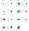 |
Fig. 1 Visual comparison of the extents of HI and star-formation vis-a-vis the stellar disc. FUV flux contours in cyan overlayed on HI column density in greyscale for sample galaxies. The ellipse over which 3.6 μm flux is extracted in Dale et al. (2009) is shown in orange. For the FUV emission the level of the first contour is arbitrarily chosen so that traces of background emission are present, and subsequent contours are in multiples of 4. The HI beams are shown at the bottom right corner of each panel. |
Since we aimed to compare our results to those found in S11, we measured the surface densities of atomic gas (Σgas,atomic), SFR and stars within the “stellar disc” – defined to be the isophote within which the 3.6 μm fluxes were determined, whose diameters are listed in Table 1. When determining all the above three quantities, a factor equal to the measured axial ratio of the Holmberg isophote (Karachentsev et al. 2013) is used to correct for the fact that we aim to measure the surface densities perpendicular to the optical disc of the galaxy and that the optical discs of such faint dwarf galaxies are oblate spheroidal in shape (Roychowdhury et al. 2013). The relative extents of the above mentioned “stellar discs” in relation to the HI and FUV emissions can be seen in Fig. 1. In all cases the “stellar disc” encompasses the star-forming region as defined by the FUV emission. But regarding the HI emission, the full range of possible variations is seen viz. the “stellar disc” being less extended, equally extended or more extended than the HI emission.
The HI total intensity maps used to measure the HI column density were constructed to have beam sizes which roughly correspond to a linear resolution of 400 pc. This is a common linear resolution at which all the galaxies from the FIGGS sample can be mapped given their varying distances and the range of baseline lengths available for our GMRT observations. It is also useful for comparison with earlier studies of the Kennisutt-Schmidt relation which were done using a similar HI resolution (see Roychowdhury et al. 2009, for examples). The HI column density is estimated by summing up the HI flux within the “stellar disc” and using the standard transformation for emission from an optically thin medium. The value is then multiplied by a factor for 1.36 to account for the presence of helium. Taking into account the calibration errors we assign a 10% error on the measured HI column densities.
For calculating the SFR from which ΣSFR is subsequently calculated, the FUV flux within the “stellar disc” is measured after masking out background and foreground sources. The SFR is then calculated using the second equation in Table 3 of Hao et al. (2011), which includes a correction for UV flux absorbed by dust and re-radiated at infrared wavelengths. The correction for dust extinction is done using 24 μm fluxes from Dale et al. (2009), as Dale et al. (2009) measure these fluxes within the ellipses identical to the “stellar disc” defined above. 24 μm fluxes are available for all galaxies listed in Table 1 except two, viz. UGC 8833 and KKH 98. For these two galaxies a 24 μm flux was approximated using Eq. (5) from Roychowdhury et al. (2014). The equation gives the best fit relation between the measured 24 μm flux and the SFRs measured using the FUV flux only, for FIGGS galaxies with both sets of fluxes available. Finally, a correction factor is applied to account for the low metallicities of the ISM in these galaxies, using values from Raiter et al. (2010) (see Roychowdhury et al. 2014, 2015, for details). We estimate the error on the measured SFRs by adding the following terms in quadrature: measurement error for FUV and 24 μm fluxes (when applicable), 10% flux calibration error for GALEX FUV data, 5% flux calibration error for Spitzer 24 μm data, and 50% error to account for the uncertainty in the SFR calibration caused by variations in the IMF and star formation history (Leroy et al. 2012, 2013).
To calculate Σ∗, we use the 3.6 μm fluxes in equation C1 from Leroy et al. (2008). They arrive at the mentioned equation by applying an empirical conversion from 3.6 μm to K-band luminosity combined with a standard K-band mass-to-light ratio. The major uncertainty comes from the assumed constant mass-to-light ratio which can be as high as 0.2 dex. Taking the other sources of uncertainty into consideration too, we use a conservative estimate of 0.3 dex error on our measured Σ∗ values.
3. Results and discussion
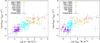 |
Fig. 2 Left panel: star formation efficiency as a function of stellar mass surface density. The different classes of galaxies from S11 are represented by differently coloured filled squares. The typical errorbars for S11 data points are represented by the black error bars. FIGGS galaxies are represented by violet circles with errorbars. The solid and dotted lies are the best fit and 1σ scatter around the best fit from S11. Right panel: star formation efficiency as a function of gas surface density. All symbols are the same as in left panel. The solid and dotted lies are the best fit and 1σ scatter around the best fit from S11 which excludes early types and LSBs. |
In the left panel of Fig. 2 where the star formation efficiency is plotted against Σ∗, our sample galaxies are over-plotted on the ESL relation along with all the galaxies from S11. Note that the points from S11 have much larger errorbars for Σgas(0.3 dex) as they have to account for the uncertainty in the CO-to-H2 conversion factor. We clearly see from the plot that dIrrs follow the ESL very well. Note that as our sample galaxies span a very limited range of Σ∗, we cannot fit a ESL-type relation only to our galaxies and compare such a fit with the ESL from S11. We do find that our sample galaxies have a mean displacement of only 0.01 dex from the best fit ESL of S11. Also, our sample galaxies have a rms scatter of 0.21 dex around the best fit relation compared to a rms scatter of 0.41 for the galaxies in S11. The right panel in Fig. 2 where the star formation efficiency is plotted against Σgas, has been included to show that our sample galaxies follow the ESL much more closely than the “canonical” Kennicutt-Schmidt relation. The right panel shows a variant of the Kennicutt-Schmidt relation with an expected linear slope of 0.4 for the “canonical” relation. In fact S11 found the slope to be 0.35 ± 0.04, after excluding the early-type and LSB galaxies which clearly do not follow the same Kennicutt-Schmidt relation as the other galaxies in their sample. Our sample galaxies have a mean deviation of 0.32 dex from the best fit KS relation by S11 in the right panel. The galaxies are clearly offset from the best fit relation towards lower star formation efficiencies similar to LSBs. The lower star formation efficiencies of dIrrs when considering the “canonical” Kennicutt-Schmidt relation has been discussed in our earlier studies (Roychowdhury et al. 2009, 2011, 2014).
In order to explain the physical reason behind the ESL, S11 considered a few possible generic frameworks of star formation. They found that an ESL-like relationship emerges based on “free-fall in a star dominated potential” for high surface brightness galaxies. Also for galaxies in which the gravitational effect of the gaseous component can be neglected “pressure-supported star formation” was found to result in power law indices as well as constants very similar to those in the ESL. Neither of these models provides an explanation as to why LSB galaxies, which are gas-dominated, should follow the ESL. It is interesting that the current study indicates that yet another kind of gas dominated galaxy, viz. dIrrs, follow the ESL.
The conclusions in S11 regarding whether pressure-supported star formation gives an ESL-like relation is based on an analytical equation of the mid-plane pressure balance from Blitz & Rosolowski (2004), which utilizes that fact that Σ∗ traces the mid-plane pressure. But the said equation from Blitz & Rosolowski (2004) is an approximation in that it was based on some necessary but simplistic assumptions. Therefore we here take a closer look at whether pressure-supported star formation can explain the ESL, given that there has been a wealth of work since which have built on Blitz & Rosolowski (2004)’s ideas of pressure-regulated molecular cloud formation. Ostriker et al. (2010) proposed a model of star formation based on atomic gas having achieved two-phase thermal and quasi-hydrostatic equilibrium, and later hydrodynamical simulations (Kim et al. 2011, 2013) have shown that these conditions are fulfilled in the atomic gas dominated regions of galaxies when turbulent and thermal pressure are regulated by supernova remnant expansion and stellar FUV heating. Other analytical laws based on feedback-regulated star formation have been able to explain the variation in KS relation across galaxies too (e.g. Dib 2011). Also recent hydrodynamical n-body simulations (Hopkins et al. 2014; Agertz & Kravtsov 2015; Orr et al. 2017) have found that feedback on local scales is crucial in setting up the KS law, independent of the recipe used for converting gas to stars, and very mildly dependant on metallicity (more on metallicity below). All these recent works point to the crucial importance of feedback from earlier generations of stars in setting up the pressure in the interstellar medium and affecting future star formation. And star formation regulated in such a manner can in principle be the reason behind the existence and universality of the ESL, as through the Σ∗ term ESL incorporates the effect of previous generations of stars.
For completeness, we next explore the consistency of ESL with an important alternative approach towards relating gas and star formation which uses the fact that metallicity is crucial to setting the atomic-to-molecular transition and thus the SFR (Krumholz et al. 2009b), and the SFE changes with the metallicity of the system. The effect is most apparent for low metallicities and at low total gas surface densities (see e.g. Fig. 1 from Krumholz 2013), which makes low metallicity galaxies ideal test cases to check the universality of the model. In Roychowdhury et al. (2015) we clearly showed that the predictions regarding the KS relation from the Ostriker et al. (2010) model better matches the resolved sub-kpc star formation law for FIGGS dIrrs and outer discs of spirals, as compared to predictions from Krumholz et al. (2009b) and Krumholz (2013). Now in this study we have shown that both LSBs and dIrrs follow the ESL, and as discussed above, feedback-regulated, pressure-supported star formation remains the most promising explanation for the ESL. It would have been ideal to know the exact prediction for the SFE-Σ∗ relation based on the feedback/pressure-regulated star formation models and the metallicity-regulated star formation models respectively, and check the predictions against the empirical ESL. Unfortunately no such predictions exist, and it is beyond the scope of this paper to work them out. Instead in order to check whether metallicity is a hidden factor behind the ESL, we check whether Σ∗ shows any correlation with metallicity.
Average metallicities of galaxies from S11.
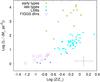 |
Fig. 3 Stellar mass surface density ploted against the average metallicity for a sub-sample of S11 and FIGGS galaxies with measured emission metallicities. The different classes of galaxies from S11 are represented by differently coloured filled squares. FIGGS galaxies are represented by violet open circles. The typical errorbars for the data points are represented by the black error bars. The dashed grey line in the background is the best-fit bivariate linear regression line (see text for details). |
We use data for galaxies from the S11 sample and from our FIGGS sample with measured emission metallicities, which can provide an indication of the average metallicity over the respective stellar discs. We have only considered galaxies from S11 which are classified as “early types”, “late types”, and “LSBs”, as these galaxies along with the FIGGS galaxies cover the low gas surface density end the ESL where the effects of metallicity should be most clearly distinguishable. For the nine FIGGS galaxies with available emission metallicity measurements, the measurements typically come from the brightest regions of these galaxies. Therefore these values can be considered as upper limits on the average metallicities over their stellar discs, although it should be noted that dwarf galaxies do not show appreciable metallicity gradients (e.g. see Westmoquette et al. 2013). We also found abundance measurements from the literature for a number of galaxies from the S11 sample which fell into one of the three categories mentioned before. These are reported in Table 2 along with the literature references. We tried to get an estimate of the average metallicity of the stellar disc of the respective galaxy wherever possible, and also accounted for the fact that the reported metallicities from different sources have different reference solar metallicity levels – which vary according to the calibration used. Wherever needed, we have used the latest measured abundance value for a galaxy. The relation between Σ∗ and the measured metallicities of these galaxies are shown in Fig. 3. We should note that we are sampling almost the entire range of Σ∗ values sampled in the full ESL. The errors on the measured metallicities mainly come from the solar reference values used. Kewley & Ellison (2008) show that the error on the solar reference for any of the standard measures of metallicity based on oxygen emission lines is at most 0.2 dex, a value we conservatively use as the estimate of the error on the measured metallicities. As we can see from Fig. 3, there is no clear relationship between Σ∗ and the average metallicities in the galaxies at the low gas surface density end of the ESL, at least definitely not a linear one. Each class of galaxies appear to be distinct from each other in the figure, with almost no overlap. Specifically, dIrrs occupy a distinct region of the Σ∗–Z space compared to the other three classes of galaxies, especially LSBs which are comparable to them in metallicity. With a bivariate linear regression fit (using the algorithm from Kelly 2007), we get a power law slope of 2.4 ± 0.2. More importantly, the algorithm estimates the standard deviation of the intrinsic random scatter of points around the best fit to be 0.73. S11 using the same algorithm found the estimated standard deviation of the intrinsic random scatter of points around the best fit ESL relation to be 0.123.
To further confirm that Σ∗ and not metallicity is the parameter which drives the star formation law, we follow S11 and try out linear regression fits (IDL regress.pro) in which we treat ΣSFR as a dependent variable. The independent variables are (i) Σgas and (ii) either of Σ∗ or metallicity. Only using the galaxies with measured metallicities (FIGGS as well as those from the S11 sample), we find the following best-fit power laws: 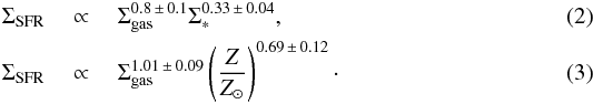 The difference between the rms scatter of residuals around the respective fits is not statistically significant, but the uncertainty on the exponent when using Z instead of Σ∗ is much larger, which reaffirms that ΣSFR has a much tighter dependence on Σ∗ compared to metallicity. We can therefore conclude that the correlation between SFE and Σ∗ (the ESL) is not driven by an underlying correlation between Σ∗ and metallicity.
S11 had shown that the Σgas–Σ∗ relation for all their sample galaxies is not tighter than the ESL (their Fig. 6), and thus ESL is not a variant of a ΣSFR–Σgas relation (KS law). This study, where low metallicity dIrrs were added to the full sample of galaxies, has helped strengthen the conclusion that ESL is an universally valid fundamental relation defining how gas converts to stars. Feedback-regulated star formation appears to be a promising candidate to explain the ESL and thus star formation across diverse classes of galaxies. It is therefore imperative for models incorporating feedback-regulated star formation, or any other model claiming to explain the conversion of gas to stars, to show that they are able to precisely predict the tight correlation that is the ESL.
Acknowledgments
We thank Ayesha Begum for providing the visibilities which were used to derive the HI maps for FIGGS galaxies used in this work. S.R. thanks Clive Dickinson for his helpful comments. S.R. acknowledges support from ERC Starting Grant No. 307209. Y.S. acknowledges the support from NSFC grant 11373021 and Jiangsu grant BK20150014. We thank the staff of the GMRT who have made the observations used in this paper possible. GMRT is run by the National Centre for Radio Astrophysics of the Tata Institute of Fundamental Research. Some of the data presented in this paper were obtained from the Multimission Archive at the Space Telescope Science Institute (MAST). STScI is operated by the Association of Universities for Research in Astronomy, Inc., under NASA contract NAS5-26555. Support for MAST for non-HST data is provided by the NASA Office of Space Science via grant NAG5-7584 and by other grants and contracts.
References
- Agertz, O., & Kravtsov, A. V. 2015, ApJ, 804, 18 [NASA ADS] [CrossRef] [Google Scholar]
- Begum, A., Chengalur, J. N., Karachentsev, I. D., Sharina, M. E., & Kaisin, S. S. 2008, MNRAS, 386, 1667 [NASA ADS] [CrossRef] [Google Scholar]
- Berg, D. A., Skillman, E. D., Marble, A. R., et al. 2012, ApJ, 754, 98 [NASA ADS] [CrossRef] [Google Scholar]
- Bigiel, F., Leroy, A., Walter, F., et al. 2008, AJ, 136, 2846 [NASA ADS] [CrossRef] [Google Scholar]
- Bigiel, F., Leroy, A., Walter, F., et al. 2010, AJ, 140, 1194 [NASA ADS] [CrossRef] [Google Scholar]
- Blitz, L., & Rosolowski, E. 2004, ApJ, 612, L29 [NASA ADS] [CrossRef] [Google Scholar]
- Blitz, L., & Rosolowski, E. 2006, ApJ, 650, 933 [NASA ADS] [CrossRef] [Google Scholar]
- Boissier, S., Prantzos, N., Boselli, A., & Gavazzi, G. 2003, MNRAS, 346, 1215 [NASA ADS] [CrossRef] [Google Scholar]
- Bolatto, A. D., Leroy, A. K., Jameson, K., et al. 2011, ApJ, 741, 12 [NASA ADS] [CrossRef] [Google Scholar]
- Daddi, E., Elbaz, D., Walter, F., et al. 2010, ApJ, 714, L118 [Google Scholar]
- Dale, D. A., Cohen, S. A., Johnson, L. C., et al. 2009, ApJ, 703, 517 [NASA ADS] [CrossRef] [Google Scholar]
- da Silva, R. L., Fumagalli, M., & Krumholz, M. R. 2014, MNRAS, 444, 3275 [NASA ADS] [CrossRef] [Google Scholar]
- Dib, S. 2011, ApJ, 737, L20 [NASA ADS] [CrossRef] [Google Scholar]
- Ekta, B., & Chengalur, J. N. 2010, MNRAS, 406, 1238 [NASA ADS] [Google Scholar]
- Elmegreen, B. G., & Hunter, D. A. 2015, ApJ, 805, 145 [NASA ADS] [CrossRef] [Google Scholar]
- Elmegreen, B. G., Rubio, M., Hunter, D. A., et al. 2013, Nature, 495, 487 [NASA ADS] [CrossRef] [Google Scholar]
- Gao, Y., & Solomon, P. M. 2004, ApJ, 606, 271 [NASA ADS] [CrossRef] [Google Scholar]
- Hao, C.-N., Kennicutt, Jr., R. C., Johnson, B. D., et al. 2011, ApJ, 741, 124 [NASA ADS] [CrossRef] [Google Scholar]
- Hopkins, P. F., Keres, D., Onorbe, J., et al. 2014, MNRAS, 445, 581 [NASA ADS] [CrossRef] [Google Scholar]
- Karachentsev, I. D., Makarov, D. I., & Kaisina, E. I. 2013, AJ, 145, 101 [NASA ADS] [CrossRef] [Google Scholar]
- Kelly, B. C. 2007, ApJ, 665, 1489 [NASA ADS] [CrossRef] [Google Scholar]
- Kennicutt, Jr., R. C. 1998, ApJ, 498, 541 [NASA ADS] [CrossRef] [Google Scholar]
- Kewley, L. J., & Ellison, S. L. 2008, ApJ, 681, 1183 [NASA ADS] [CrossRef] [Google Scholar]
- Kim, C.-G., Kim, W.-T., & Ostriker, E. C. 2011, ApJ, 743, 25 [NASA ADS] [CrossRef] [Google Scholar]
- Kim, C.-G., Ostriker, E. C., & Kim, W.-T. 2013, ApJ, 776, 1 [NASA ADS] [CrossRef] [Google Scholar]
- Krumholz, M. R. 2013, MNRAS, 436, 2747 [NASA ADS] [CrossRef] [Google Scholar]
- Krumholz, M. R., McKee, C. F., & Tumlinson, J. 2009a, ApJ, 693, 216 [NASA ADS] [CrossRef] [Google Scholar]
- Krumholz, M. R., McKee, C. F., & Tumlinson, J. 2009b, ApJ, 699, 850 [NASA ADS] [CrossRef] [Google Scholar]
- Lada, C. J. 2015, Galaxies in 3D across the Universe, 309, 31 [NASA ADS] [Google Scholar]
- Leroy, A. K., Walter, F., Brinks, E., et al. 2008, AJ, 136, 2782 [NASA ADS] [CrossRef] [Google Scholar]
- Leroy, A. K., Bigiel, F., de Blok, W. J. G., et al. 2012, AJ, 144, 3 [NASA ADS] [CrossRef] [Google Scholar]
- Leroy, A. K., Walter, F., Sandstrom, K., et al. 2013, AJ, 146, 19 [NASA ADS] [CrossRef] [Google Scholar]
- Marble, A. R., Engelbracht, C. W., van Zee, L., et al. 2010, ApJ, 715, 506 [NASA ADS] [CrossRef] [Google Scholar]
- McDermid, R. M., Alatalo, K., Blitz, L., et al. 2015, MNRAS, 448, 3484 [NASA ADS] [CrossRef] [Google Scholar]
- Moustakas, J., Kennicutt, Jr., R. C., Tremonti, C. A., et al. 2010, ApJS, 190, 233 [NASA ADS] [CrossRef] [Google Scholar]
- Orr, M., Hayward, C., Hopkins, P., et al. 2017, MNRAS, submitted [arXiv:1701.01788] [Google Scholar]
- Ostriker, E. C., McKee, C. F., & Leroy, A. K. 2010, ApJ, 721, 975 [NASA ADS] [CrossRef] [Google Scholar]
- Pilyugin, L. S., Grebel, E. K., & Kniazev, A. Y. 2014, AJ, 147, 131 [NASA ADS] [CrossRef] [Google Scholar]
- Raiter, A., Schaerer, D., & Fosbury, R. A. E. 2010, A&A, 523, 64 [Google Scholar]
- Roychowdhury, S., Chengalur, J. N., Begum, A., & Karachentsev, I. D. 2009, MNRAS, 397, 1435 [NASA ADS] [CrossRef] [Google Scholar]
- Roychowdhury, S., Chengalur, J. N., Kaisin, S. S., Begum, A., & Karachentsev, I. D. 2011, MNRAS, 414, L55 [NASA ADS] [CrossRef] [Google Scholar]
- Roychowdhury, S., Chengalur, J. N., Karachentsev, I. D., & Kaisina, E. I. 2013, MNRAS, 436, L104 [NASA ADS] [CrossRef] [Google Scholar]
- Roychowdhury, S., Chengalur, J. N., Kaisin, S. S., & Karachentsev, I. D. 2014, MNRAS, 445, 1392 [NASA ADS] [CrossRef] [Google Scholar]
- Roychowdhury, S., Huang, M.-L., Kauffmann, G., Wang, J., & Chengalur, J. N. 2015, MNRAS, 449, 3700 [NASA ADS] [CrossRef] [Google Scholar]
- Ryder, S. D., & Dopita, M. A. 1994, ApJ, 430, 142 [NASA ADS] [CrossRef] [Google Scholar]
- Schmidt, M. 1959, ApJ, 129, 243 [NASA ADS] [CrossRef] [Google Scholar]
- Shetty, R., Kelly, B. C., Rahman, N., et al. 2014, MNRAS, 437, L61 [NASA ADS] [CrossRef] [Google Scholar]
- Shi, Y., Helou, G., Yan, L., et al. 2011, ApJ, 733, 87 [NASA ADS] [CrossRef] [Google Scholar]
- Shi, Y., Armus, L., Helou, G., et al. 2014, Nature, 514, 335 [NASA ADS] [CrossRef] [Google Scholar]
- Shi, Y., Wang, J., Zhang, Z.-Y., et al. 2016, Nat. Comm., 7, 13789 [Google Scholar]
- Sternberg, A., Le Petit, F., Roueff, E., & Le Bourlot, J. 2014, ApJ, 790, 10 [NASA ADS] [CrossRef] [MathSciNet] [Google Scholar]
- Westmoquette, M. S., James, B., Monreal-Ibero, A., & Walsh, J. R. 2013, A&A, 550, A88 [NASA ADS] [CrossRef] [EDP Sciences] [Google Scholar]
- Wyder, T. K., Martin, D. C., Barlow, T. A., et al. 2009, ApJ, 696, 1834 [NASA ADS] [CrossRef] [Google Scholar]
All Tables
All Figures
|
Fig. 1 Visual comparison of the extents of HI and star-formation vis-a-vis the stellar disc. FUV flux contours in cyan overlayed on HI column density in greyscale for sample galaxies. The ellipse over which 3.6 μm flux is extracted in Dale et al. (2009) is shown in orange. For the FUV emission the level of the first contour is arbitrarily chosen so that traces of background emission are present, and subsequent contours are in multiples of 4. The HI beams are shown at the bottom right corner of each panel. |
| In the text | |
|
Fig. 2 Left panel: star formation efficiency as a function of stellar mass surface density. The different classes of galaxies from S11 are represented by differently coloured filled squares. The typical errorbars for S11 data points are represented by the black error bars. FIGGS galaxies are represented by violet circles with errorbars. The solid and dotted lies are the best fit and 1σ scatter around the best fit from S11. Right panel: star formation efficiency as a function of gas surface density. All symbols are the same as in left panel. The solid and dotted lies are the best fit and 1σ scatter around the best fit from S11 which excludes early types and LSBs. |
| In the text | |
|
Fig. 3 Stellar mass surface density ploted against the average metallicity for a sub-sample of S11 and FIGGS galaxies with measured emission metallicities. The different classes of galaxies from S11 are represented by differently coloured filled squares. FIGGS galaxies are represented by violet open circles. The typical errorbars for the data points are represented by the black error bars. The dashed grey line in the background is the best-fit bivariate linear regression line (see text for details). |
| In the text | |
Current usage metrics show cumulative count of Article Views (full-text article views including HTML views, PDF and ePub downloads, according to the available data) and Abstracts Views on Vision4Press platform.
Data correspond to usage on the plateform after 2015. The current usage metrics is available 48-96 hours after online publication and is updated daily on week days.
Initial download of the metrics may take a while.